On a partial theta function and its spectrum

Abstract

The bivariate series $\theta(q,x):=\sum_{j=0}^{\infty}q^{j(j+1)/2}x^{j}$ defines a partial theta function. For fixed $q$ ($|q|<1$), $\theta(q,.)$ is an entire function. For $q\in(-1,0)$ the function $\theta(q,.)$ has infinitely many negative and infinitely many positive real zeros. There exists a sequence $\{\bar{q}_{j}\}$ of values of $q$ tending to $-1^{+}$ such that $\theta(\bar{q}_{k},.)$ has a double real zero $\bar{y}_{k}$ (the rest of its real zeros being simple). For $k$ odd (resp. for $k$ even) $\theta(\bar{q}_{k},.)$ has a local minimum at $\bar{y}_{k}$ and $\bar{y}_{k}$ is the rightmost of the real negative zeros of $\theta(\bar{q}_{k},.)$ (resp. $\theta(\bar{q}_{k},.)$ has a local maximum at $\bar{y}_{k}$ and for $k$ sufficiently large $\bar{y}_{k}$ is the second from the left of the real negative zeros of $\theta(\bar{q}_{k},.)$). For $k$ sufficiently large one has $-1<\bar{q}_{k+1}<\bar{q}_{k}<0$. One has $\bar{q}_{k}=1-(\pi/8k)+o(1/k)$ and $|\bar{y}_{k}|\rightarrow e^{\pi/2}=4.810477382\ldots$.

AMS classification: 26A06

Keywords: partial theta function; spectrum

1 Introduction

The bivariate series $\theta(q,x):=\sum_{j=0}^{\infty}q^{j(j+1)/2}x^{j}$ defines an entire function in $x$ for every fixed $q$ from the open unit disk. This function is called a partial theta function because $\theta(q^{2},x/q)=\sum_{j=0}^{\infty}q^{j^{2}}x^{j}$ whereas the Jacobi theta function is defined by the same series, but when summation is performed from $-\infty$ to $\infty$ (i.e. when summation is not partial).

There are several domains in which the function $\theta$ finds applications: in the theory of (mock) modular forms (see [3]), in statistical physics and combinatorics (see [18]), in asymptotic analysis (see [2]) and in Ramanujan type $q$-series (see [19]). Recently it has been considered in the context of problems about hyperbolic polynomials (i.e. real polynomials having all their zeros real, see [4], [16], [5], [15], [6], [13] and [9]). These problems have been studied earlier by Hardy, Petrovitch and Hutchinson (see [4], [5] and [16]). For more information about $\theta$, see also [1].

For $q\in\mathbb{C}$, $|q|\leq 0.108$, the function $\theta(q,.)$ has no multiple zeros, see [11]. For $q\in[0,1)$ the function $\theta$ has been studied in [13], [8], [9] and [10]. The results are summarized in the following theorem:

Theorem 1.

(1) For any $q\in(0,1)$ the function $\theta(q,.)$ has infinitely many negative zeros.

(2) There exists a sequence of values of $q$ (denoted by $0<\tilde{q}_{1}<\tilde{q}_{2}<\cdots$) tending to $1^{-}$ such that $\theta(\tilde{q}_{k},.)$ has a double negative zero $y_{k}$ which is the rightmost of its real zeros and which is a local minimum of $\theta(q,.)$. One has $\tilde{q}_{1}=0.3092493386\ldots$.

(3) For the remaining values of $q\in[0,1)$ the function $\theta(q,.)$ has no multiple real zero.

(4) For $q\in(\tilde{q}_{k},\tilde{q}_{k+1})$ (we set $\tilde{q}_{0}=0$) the function $\theta(q,.)$ has exactly $k$ complex conjugate pairs of zeros counted with multiplicity.

(5) One has $\tilde{q}_{k}=1-(\pi/2k)+o(1/k)$ and $y_{k}\rightarrow-e^{\pi}=-23.1407\ldots$.

Definition 2.

A value of $q\in\mathbb{C}$, $|q|<1$, is said to belong to the spectrum of $\theta$ if $\theta(q,.)$ has a multiple zero.

In the present paper we consider the function $\theta$ in the case when $q\in(-1,0]$. In order to use the results about the case $q\in[0,1)$ one can notice the following fact. For $q\in(-1,0]$ set $v:=-q$. Then

$$\theta(q,x)=\theta(-v,x)=\theta(v^{4},-x^{2}/v)-vx\theta(v^{4},-vx^{2})~{}.$$ (1)

We prove the analog of the above theorem. The following three theorems are proved respectively in Sections 3, 4 and 5.

Theorem 3.

For any $q\in(-1,0)$ the function $\theta(q,.)$ has infinitely many negative and infinitely many positive real zeros.

Theorem 4.

(1) There exists a sequence of values of $q$ (denoted by $\bar{q}_{j}$) tending to $-1^{+}$ such that $\theta(\bar{q}_{k},.)$ has a double real zero $\bar{y}_{k}$ (the rest of its real zeros being simple). For the remaining values of $q\in(-1,0)$ the function $\theta(q,.)$ has no multiple real zero.

(2) For $k$ odd (resp. for $k$ even) one has $\bar{y}_{k}<0$, $\theta(\bar{q}_{k},.)$ has a local minimum at $\bar{y}_{k}$ and $\bar{y}_{k}$ is the rightmost of the real negative zeros of $\theta(\bar{q}_{k},.)$ (resp. $\bar{y}_{k}>0$, $\theta(\bar{q}_{k},.)$ has a local maximum at $\bar{y}_{k}$ and for $k$ sufficiently large $\bar{y}_{k}$ is the leftmost but one (second from the left) of the real negative zeros of $\theta(\bar{q}_{k},.)$).

(3) For $k$ sufficiently large one has $-1<\bar{q}_{k+1}<\bar{q}_{k}<0$.

(4) For $k$ sufficiently large and for $q\in(\bar{q}_{k+1},\bar{q}_{k})$ the function $\theta(q,.)$ has exactly $k$ complex conjugate pairs of zeros counted with multiplicity.

Remark 5.

Numerical experience confirms the conjecture that parts (2), (3) and (4) of the theorem are true for any $k\in\mathbb{N}$. Proposition 14 clarifies part (2) of the theorem.

Theorem 6.

One has $\bar{q}_{k}=1-(\pi/8k)+o(1/k)$ and $|\bar{y}_{k}|\rightarrow e^{\pi/2}=4.810477382\ldots$.

Remarks 7.

(1) Theorems 1 and 4 do not tell whether there are values of $q\in(-1,1)$ for which $\theta(q,.)$ has a multiple complex conjugate pair of zeros.

(2) It would be interesting to know whether the sequences $\{y_{k}\}$ and $\{\bar{y}_{2k-1}\}$ are monotone decreasing and $\{\bar{y}_{2k}\}$ is monotone increasing. This is true for at least the five first terms of each sequence.

(3) It would be interesting to know whether there are complex non-real values of $q$ of the open unit disk belonging to the spectrum of $\theta$ and (as suggested by A. Sokal) whether $|\tilde{q}_{1}|$ is the smallest of the moduli of the spectral values.

(4) The following statement is formulated and proved in [7]:

The sum of the series $\sum_{j=0}^{\infty}q^{j(j+1)/2}x^{j}$ (considered for $q\in(0,1)$ and $x\in\mathbb{C}$) tends to $1/(1-x)$ (for $x$ fixed and as $q\rightarrow 1^{-}$) exactly when $x$ belongs to the interior of the closed Jordan curve $\{e^{|s|+is},s\in[-\pi,\pi]\}$.

This statement and equation (1) imply that as $q\rightarrow-1^{+}$, $\theta(q,x)\rightarrow(1-x)/(1+x^{2})$ for $x\in(-e^{\pi/2},e^{\pi/2})$, $e^{\pi/2}=4.810477381\ldots$. Notice that the radius of convergence of the Taylor series at $0$ of the function $(1-x)/(1+x^{2})$ equals 1.

(5) On Fig. 1 and 2 we show the graphs of $\theta(\bar{q}_{k},.)$ for $k=1$, $\ldots$, $8$. The ones for $k=1$, $2$, $5$ and $6$ are shown in black, the others are drawn in grey. One can notice by looking at Fig. 2 that for $x\in[-2.5,2.5]$ the graphs of $\theta(\bar{q}_{k},.)$ for $k\geq 5$ are hardly distinguishable from the one of $(1-x)/(1+x^{2})$.

(6) The approximative values of $\bar{q}_{k}$ and $\bar{y}_{k}$ for $k=1$, $2$, $\ldots$ $8$ are:

$$\begin{array}[]{rcccccccc}k&{}{}{}{}{}\hfil&1&{}{}\hfil&2&{}{}\hfil&3&{}{}\hfil&4\\ -\bar{q}_{k}&{}{}{}{}{}\hfil&0.72713332&{}{}\hfil&0.78374209&{}{}\hfil&0.84160192&{}{}\hfil&0.86125727\\ \bar{y}_{k}&{}{}{}{}{}\hfil&-2.991&{}{}\hfil&2.907&{}{}\hfil&-3.621&{}{}\hfil&3.523\\ \\ k&{}{}{}{}{}\hfil&5&{}{}\hfil&6&{}{}\hfil&7&{}{}\hfil&8\\ -\bar{q}_{k}&{}{}{}{}{}\hfil&0.88795282&{}{}\hfil&0.89790438&{}{}\hfil&0.913191{}{}&{}{}\hfil&0.9192012{}\\ \bar{y}_{k}&{}{}{}{}{}\hfil&-3.908&{}{}\hfil&3.823&{}{}\hfil&-4.08{}&{}{}\hfil&4.002\end{array}$$

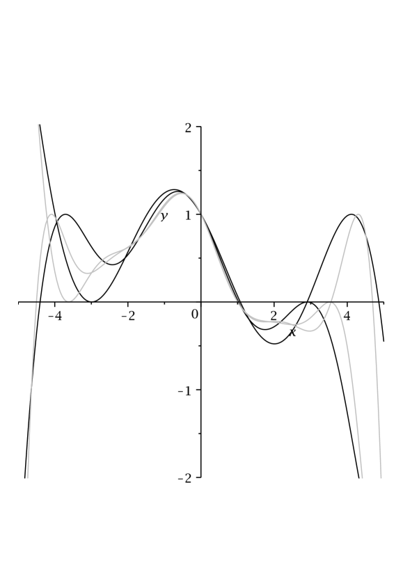
Figure 1: The graphs of the functions $\theta(\bar{q}_{k},.)$ for $k=1$, $2$, $3$ and $4$.

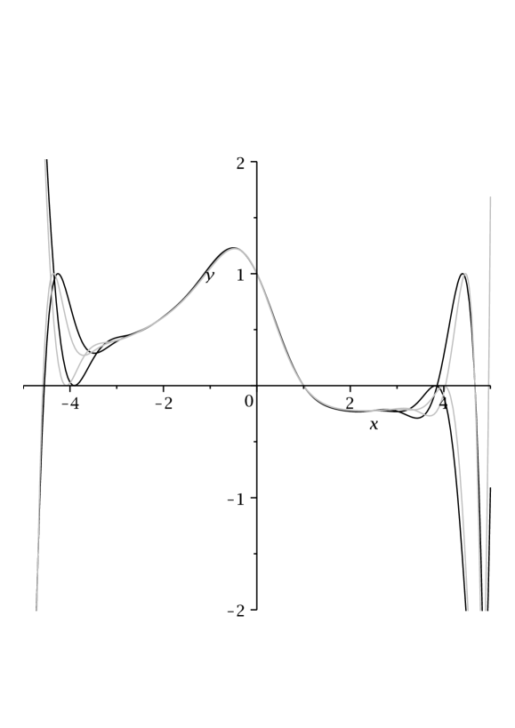
Figure 2: The graphs of the functions $\theta(\bar{q}_{k},.)$ for $k=5$, $6$, $7$ and $8$.

2 Some facts about $\theta$

This section contains properties of the function $\theta$, known or proved in [9]. When a property is valid for all $q$ from the unit disk or for all $q\in(-1,1)$, we write $\theta(q,x)$. When a property holds true only for $q\in[0,1)$ or only for $q\in(-1,0]$, we write $\theta(v,x)$ or $\theta(-v,x)$, where $v\in[0,1)$.

Theorem 8.

(1) The function $\theta$ satisfies the following functional equation:

$$\theta(q,x)=1+qx\theta(q,qx)$$ (2)

and the following differential equation:

$$2q\partial\theta/\partial q=2x\partial\theta/\partial x+x^{2}\partial^{2}\theta/\partial x^{2}=x\partial^{2}(x\theta)/\partial x^{2}$$ (3)

(2) For $k\in\mathbb{N}$ one has $\theta(v,-v^{-k})\in(0,v^{k})$.

(3) In the following two situations the two conditions sgn$(\theta(v,-v^{-k-1/2}))=(-1)^{k}$ and $|\theta(v,-v^{-k-1/2})|>1$ hold true:

(i) For $k\in\mathbb{N}$ and $v>0$ small enough;

(ii) For any $v\in(0,1)$ fixed and for $k\in\mathbb{N}$ large enough.

The real entire function $\psi(z)$ is said to belong to the Laguerre-Pólya class ${\cal L-P}$ if it can be represented as

$$\psi(x)=cx^{m}e^{-\alpha x^{2}+\beta x}\prod_{k=1}^{\omega}(1+x/x_{k})e^{-x/x_{k}},$$

where $\omega$ is a natural number or infinity, $c$, $\beta$ and $x_{k}$ are real, $\alpha\geq 0$, $m$ is a nonnegative integer and $\sum x_{k}^{-2}<\infty$. Similarly, the real entire function $\psi_{*}(x)$ is a function of type I in the Laguerre-Pólya class, written $\psi_{*}\in{\cal L-PI}$, if $\psi_{*}(x)$ or $\psi_{*}(-x)$ can be represented in the form

$$\psi_{*}(x)=cx^{m}e^{\sigma x}\prod_{k=1}^{\omega}(1+x/x_{k}),$$ (4)

where $c$ and $\sigma$ are real, $\sigma\geq 0$, $m$ is a nonnegative integer, $x_{k}>0$, and $\sum 1/x_{k}<\infty$. It is clear that ${\cal L-PI}\subset{\cal L-P}$. The functions in ${\cal L-P}$, and only these, are uniform limits, on compact subsets of $\mathbb{C}$, of hyperbolic polynomials (see, for example, Levin [14, Chapter 8]). Similarly, $\psi\in{\cal L-PI}$ if and only if $\psi$ is a uniform limit on the compact sets of the complex plane of polynomials whose zeros are real and are either all positive, or all negative. Thus, the classes ${\cal L-P}$ and ${\cal L-PI}$ are closed under differentiation; that is, if $\psi\in{\cal L-P}$, then $\psi^{(\nu)}\in{\cal L-P}$ for every $\nu\in\mathbb{N}$ and similarly, if $\psi\in{\cal L-PI}$, then $\psi^{(\nu)}\in{\cal L-PI}$ . Pólya and Schur [17] proved that if

$$\psi(x)=\sum_{k=0}^{\infty}\gamma_{k}\frac{x^{k}}{k!}$$ (5)

belongs to ${\cal L-P}$ and its Maclaurin coefficients $\gamma_{k}=\psi^{(k)}(0)$ are all nonnegative, then $\psi\in{\cal L-PI}$.

The following theorem is the basic result contained in [12]:

Theorem 9.

(1) For any fixed $q\in\mathbb{C}^{*}$, $|q|<1$, and for $k$ sufficiently large, the function $\theta(q,.)$ has a zero $\zeta_{k}$ close to $-q^{-k}$ (in the sense that $|\zeta_{k}+q^{-k}|\rightarrow 0$ as $k\rightarrow\infty$). These are all but finitely-many of the zeros of $\theta$.

(2) For any $q\in\mathbb{C}^{*}$, $|q|<1$, one has $\theta(q,x)=\prod_{k}(1+x/x_{k})$, where $-x_{k}$ are the zeros of $\theta$ counted with multiplicity.

(3) For $q\in(\tilde{q}_{j},\tilde{q}_{j+1}]$ the function $\theta(q,.)$ is a product of a degree $2j$ real polynomial without real roots and a function of the Laguerre-Pólya class $\cal{L-PI}$. Their respective forms are $\prod_{k=1}^{2j}(1+x/\eta_{k})$ and $\prod_{k}(1+x/\xi_{k})$, where $-\eta_{k}$ and $-\xi_{k}$ are the complex and the real zeros of $\theta$ counted with multiplicity.

(4) For any fixed $q\in\mathbb{C}^{*}$, $|q|<1$, the function $\theta(q,.)$ has at most finitely-many multiple zeros.

(5) For any $q\in(-1,0)$ the function $\theta(q,.)$ is a product of the form $R(q,.)\Lambda(q,.)$, where $R=\prod_{k=1}^{2j}(1+x/\tilde{\eta}_{k})$ is a real polynomial with constant term $1$ and without real zeros and $\Lambda=\prod_{k}(1+x/\tilde{\xi}_{k})$, $\tilde{\xi}_{k}\in\mathbb{R}^{*}$, is a function of the Laguerre-Pólya class $\cal{L-P}$. One has $\tilde{\xi}_{k}\tilde{\xi}_{k+1}<0$. The sequence $\{|\tilde{\xi}_{k}|\}$ is monotone increasing for $k$ large enough.

3 Proof of Theorem 3

One can use equation (1). By part (3) of Theorem 8 with $v^{4}$ for $v$, for each $v\in(0,1)$ fixed and for $k$ large enough, if $-x^{2}/v=-(v^{4})^{-k-1/2}$ (i.e. if $|x|=v^{-2k-1/2}$), then $|\theta(v^{4},-x^{2}/v)|>1$ and sgn$(\theta(v^{4},-x^{2}/v))=(-1)^{k}$. At the same time part (2) of Theorem 8 implies that for $-vx^{2}=-(v^{4})^{-k}$ (i.e. again for $|x|=v^{-2k-1/2}$) one has $\theta(v^{4},-vx^{2})\in(0,v^{4k})$ hence $|vx\theta(v^{4},-vx^{2})|<v^{2k+1/2}<1$. This means that for $v\in(0,1)$ fixed and for $k$ large enough the equality sgn$(\theta(v^{4},-x^{2}/v))=(-1)^{k}$ holds, i.e. there is a zero of $\theta$ on each interval of the form $(-v^{-2k-1/2},-v^{-2k+1/2})$ and $(v^{-2k+1/2},v^{-2k-1/2})$.

4 Proof of Theorem 4

4.1 Properties of the zeros of $\theta$

The present subsection contains some preliminary information about the zeros of $\theta$.

Lemma 10.

For $q\in[-0.108,0)$ all zeros of $\theta(q,.)$ are real and distinct.

Proof.

Indeed, it is shown in [11] that for $q\in\mathbb{C}$, $|q|\leq 0.108$, the zeros of $\theta$ are of the form $-q^{-j}\Delta_{j}$, $\Delta_{j}\in[0.2118,1.7882]$. This implies (see [11]) that the moduli of all zeros are distinct for $|q|\leq 0.108$. When $q$ is real, then as all coefficients of $\theta$ are real, each of its zeros is either real or belongs to a complex conjugate pair. The moduli of the zeros being distinct the zeros are all real and distinct. ∎

Notation 11.

We denote by $0<x_{1}<x_{3}<\cdots$ the positive and by $\cdots<x_{4}<x_{2}<0$ the negative zeros of $\theta$. For $q\in[-0.108,0)$ this notation is in line with the fact that $x_{j}$ is close to $-q^{-j}$.

Remarks 12.

(1) The quantities $\Delta_{j}$ are constructed in [11] as convergent Taylor series in $q$ of the form $1+O(q)$.

(2) For $q\in(-1,0)$ the function $\theta(q,.)$ has no zeros in $[-1,0)$. Indeed, this follows from

$$\theta=1+q^{3}x^{2}+q^{10}x^{4}+\cdots+qx(1+q^{5}x^{2}+q^{14}x^{4}+\cdots)~{}.$$

Each of the two series is sign-alternating, with positive first term and with decreasing moduli of its terms for $q\in(-1,0)$, $x\in[-1,0)$. Hence their sums are positive; as $qx>0$, one has $\theta>0$.

Lemma 13.

For $q\in[-0.108,0)$ the real zeros of $\theta$ and their products with $q$ are arranged on the real line as shown on Fig. 3.

Proof.

The lemma follows from equation (2). Indeed,

$$0=\theta(q,x_{4k+2})=1+qx_{4k+2}\theta(q,qx_{4k+2})~{}~{},~{}~{}x_{4k+2}<0~{}~{}{\rm and}~{}~{}q<0~{}~{}{\rm hence}~{}~{}\theta(q,qx_{4k+2})<0~{}.$$

For small values of $q$ the quantity $qx_{4k+2}$ is close to $-q^{-4k-1}$ (see Lemma 10 and part (1) of Remarks 12), i.e. close to $x_{4k+1}$ and as $\theta(q,qx_{4k+2})<0$, one must have $x_{4k+1}<qx_{4k+2}<x_{4k+3}$. By continuity these inequalities hold for all $q<0$ for which the zeros $x_{4k+1}<x_{4k+3}$ are real and distinct.

In the same way one can justify the disposition of the other points of the form $qx_{j}$ w.r.t. the points $x_{j}$. ∎

Figure 3: The real zeros of $\theta$ for $q\in(-1,0)$.

Proposition 14.

The function $\theta(q,.)$ with $q\in(-1,0)$ has a zero in the interval $(0,-1/q)$. More precisely, one has $\theta(q,-1/q)<0$.

Proof.

Setting as above $v=-q$ one gets

$$\theta(-v,1/v)=-v\Phi(v)+v^{3}\Psi(v)~{}~{},~{}~{}{\rm where}~{}~{}\Phi(v)=\sum_{j=0}^{\infty}(-1)^{j}v^{2j^{2}+3j}~{}~{},~{}~{}\Psi(v)=\sum_{j=0}^{\infty}(-1)^{j}v^{2j^{2}+5j}~{}.$$

Further we use some results of [9]. Consider the functions $\varphi_{k}(\tau):=\sum_{j=0}^{\infty}(-1)^{j}\tau^{kj+j(j-1)/2}=\theta(\tau,-\tau^{k-1})$ and $\xi_{k}(\tau):=1/(1+\tau^{k})$, $\tau\in[0,1)$, $k>0$.

Proposition 15.

(1) The functions $\varphi_{k}$ are real analytic on $[0,1)$; when $k>0$, then $\varphi_{k}<\xi_{k}$; when $k>1$, then $\varphi_{k}>\xi_{k-1}$; one has $\lim_{\tau\rightarrow 1^{-}}\varphi_{k}(\tau)=1/2$.

(2) Consider the function $\varphi_{k}$ as a function of the two variables $(k,\tau)$. One has $\partial\varphi_{k}/\partial k>0$ for $k>0$.

(3) For $q\in(0,1)$, $x\in(-q^{-1},\infty)$ one has $\partial\theta/\partial x>0$.

(4) For $q\in(0,1)$, $x\in(-q^{-1/2},\infty)$ one has $\theta>1/2$.

Before proving Proposition 15 we finish the proof of Proposition 14. Part (2) of Proposition 15 implies $\varphi_{3/4}(v^{4})>\varphi_{1/4}(v^{4})$. As $-v\Phi(v)=\varphi_{1/4}(v^{4})-1$ and $-v^{3}\Psi(v)=\varphi_{3/4}(v^{4})-1$, this means that $\theta(-v,1/v)<0$, i.e. $\theta(q,-1/q)<0$. ∎

Proof of Proposition 15:.

Part (1) of the proposition is proved in [9].

To prove part (2) observe that

$$\begin{array}[]{rcl}\partial\varphi_{k}/\partial k&=&(-\log\tau)\sum_{j=1}^{\infty}(-1)^{j-1}j\tau^{kj+j(j-1)/2}\\ \\ &=&(-\log\tau)\tau^{k}\sum_{j=1}^{\infty}(\varphi_{k+j}-\tau^{k+j}\varphi_{k+j+1})\end{array}$$

As $\varphi_{k+j}-\tau^{k+j}\varphi_{k+j+1}=2\varphi_{k+j}-1$ and (see part (1) of the proposition) as $\varphi_{k+j}(\tau)>\xi_{k+j-1}(\tau)\geq 1/2$, each difference $\varphi_{k+j}-\tau^{k+j}\varphi_{k+j+1}$ is positive on $[0,1)$. The factors $-\log\tau$ and $\tau^{k}$ are also positive.

For $x\in(-q^{-1},0]$ part (3) follows from part (2) and from $\varphi_{k}(\tau)=\theta(\tau,-\tau^{k-1})$. Indeed, one can represent $x$ as $-\tau^{k-1}$ for some $k>0$; for fixed $\tau$, as $x$ increases, $k$ also increases. One has

$$0<\partial\varphi_{k}/\partial k=(-\log\tau)\partial\theta/\partial x|_{x=-\tau^{k-1}}~{}~{}{\rm and}~{}~{}-\log\tau>0~{}.$$

For $x>0$ part (3) results from all coefficients of $\theta(v,x)$ considered as a series in $x$ being positive.

For $x\in(-q^{-1/2},0]$ part (4) follows from part (3). Indeed, consider the function $\psi:=1+2\sum_{j=1}^{\infty}(-1)^{j}\tau^{j^{2}}$, $\tau\in[0,1)$. This function is positive valued, decreasing and tending to $0$ as $\tau\rightarrow 1^{-}$, see [8]. As $0<\psi(\tau^{1/2})/2=\varphi_{1/2}(\tau)-1/2$, for $k\geq 1/2$ part (2) of Proposition 15 implies

$$\theta(\tau,-\tau^{k-1})=\varphi_{k}(\tau)\geq\varphi_{1/2}(\tau)>1/2~{}.$$

For $x=0$ one has $\theta=1$ hence for $x>0$ part (4) follows from part (2). ∎

The following lemma follows immediately from the result of V. Katsnelson cited in part (4) of Remarks 7 and from Proposition 14:

Lemma 16.

For any $\varepsilon>0$ sufficiently small there exists $\delta>0$ such that for $q\in(-1,-1+\delta]$ the function $\theta(q,.)$ has a single real zero in the interval $(-e^{\pi/2}+\varepsilon,e^{\pi/2}-\varepsilon)$. This zero is simple and positive.

4.2 How do the zeros of $\theta$ coalesce?

Further we describe the way multiple zeros are formed when $q$ decreases from $0$ to $-1$.

Definition 17.

We say that the phenomenon A happens before the phenomenon B if A takes place for $q=q_{1}$, B takes place for $q=q_{2}$ and $-1<q_{2}<q_{1}<0$. By phenomena we mean that certain zeros of $\theta$ or another function coalesce.

Notation 18.

We denote by $x_{j}\prec x_{k}$ the following statement: The zeros $x_{k}$ and $x_{k+2}$ of $\theta$ can coalesce only after $x_{j}$ and $x_{j+2}$ have coalesced.

Lemma 19.

One has $x_{4k+2}\prec x_{4k+3}$, $x_{4k+2}\prec x_{4k+1}$, $x_{4k+3}\prec x_{4k+4}$ and $x_{4k+5}\prec x_{4k+4}$, $k\in\mathbb{N}\cup 0$.

Proof.

The statements follow respectively from

$$\begin{array}[]{lcll}qx_{4k+5}<x_{4k+4}<x_{4k+2}<qx_{4k+3}&,&x_{4k+1}<qx_{4k+2}<qx_{4k+4}<x_{4k+3}&,\\ \\ qx_{4k+4}<x_{4k+3}<x_{4k+5}<qx_{4k+6}&~{}~{}{\rm and{}{}}&x_{4k+6}<qx_{4k+7}<qx_{4k+5}<x_{4k+4}&.\end{array}$$

∎

Lemma 20.

One has $x_{4k+2}\prec x_{4k+6}$, $k\in\mathbb{N}\cup 0$.

Proof.

Indeed, equation (2) implies the following one:

$$\theta(q,x)=1+qx+q^{3}x^{2}+q^{6}x^{3}+q^{10}x^{4}\theta(q,q^{4}x)~{}.$$ (6)

For $x=x_{4k+2}/q^{4}$ one obtains

$$\theta(q,x_{4k+2}/q^{4})=1+x_{4k+2}/q^{3}+x_{4k+2}^{2}/q^{5}+x_{4k+2}^{3}/q^{6}=(1+x_{4k+2}^{2}/q^{5})+(x_{4k+2}/q^{3}+x_{4k+2}^{3}/q^{6})~{}.$$

Each of the two sums is negative due to $q\in(-1,0)$, $x_{4k+2}<-1$ (see part (2) of Remarks 12). For small values of $|q|$ one has $x_{4k+2}/q^{4}\in(x_{4k+8},x_{4k+6})$ because $x_{j}=-q^{-j}(1+O(q))$ and $\theta(q,x_{4k+2}/q^{4})<0$. By continuity this holds true for all $q\in(-1,0)$ for which the zeros $x_{4k+8}$, $x_{4k+6}$, $x_{4k+4}$ and $x_{4k+2}$ are real and distinct. Hence if $x_{4k+2}$ and $x_{4k+4}$ have not coalesced, then $x_{4k+6}$ and $x_{4k+8}$ are real and distinct. ∎

Remarks 21.

(1) Recall that for $q\in(-1,0)$ we set $v:=-q$ and that equation (1) holds true.

(2) Equation (3) implies that the values of $\theta$ at its local maxima decrease and its values at local minima increase as $q$ decreases in $(-1,0)$. Indeed, at a critical point one has $\partial\theta/\partial x=0$, so $2q\partial\theta/\partial q=x^{2}\partial^{2}\theta/\partial x^{2}$. At a minimum one has $\partial^{2}\theta/\partial x^{2}\geq 0$, so $\partial\theta/\partial q\leq 0$ and the value of $\theta$ increases as $q$ decreases; similarly for a maximum.

(3) In particular, this means that $\theta$ can only lose real zeros, but not acquire such as $q$ decreases on $(-1,0)$. Indeed, the zeros of $\theta$ depend continuously on $q$. If at some point of the real axis a new zero of even multiplicity appears, then it cannot be a maximum because the critical value must decrease and it cannot be a minimum because its value must increase.

(4) To treat the cases of odd multiplicities of the zeros it suffices to differentiate both sides of equation (3) w.r.t. $x$. For example, a simple zero $x_{0}$ of $\theta$ cannot become a triple one because

$$2q\partial/\partial q(\partial\theta/\partial x)=2\partial\theta/\partial x+4x\partial^{2}\theta/\partial x^{2}+x^{2}\partial^{3}\theta/\partial x^{3}$$

which means that as $\partial\theta/\partial x|_{x=x_{0}}=\partial^{2}\theta/\partial x^{2}|_{x=x_{0}}=0$, then either $\partial^{3}\theta/\partial x^{3}|_{x=x_{0}}>0$ hence in a neighbourhood of $x_{0}$ one has $\partial\theta/\partial x\geq 0$ and $\partial/\partial q(\partial\theta/\partial x)<0$, or $\partial^{3}\theta/\partial x^{3}|_{x=x_{0}}<0$ hence $\partial\theta/\partial x\leq 0$ and $\partial/\partial q(\partial\theta/\partial x)>0$ (in a neighbourhood of $x_{0}$), so in both cases the triple zero bifurcates into a simple one and a complex pair as $q$ decreases. The case of a zero of multiplicity $2m+1$, $m\in\mathbb{N}$, is treated by analogy.

(5) In equation (1) the first argument (i.e. $v^{4}$) of both functions $\theta(v^{4},-x^{2}/v)$ and $\theta(v^{4},-vx^{2})$ is the same, so when one of them has a double zero, then they both have double zeros. If the double zero of the first one is at $x=a$, then the one of the second is at $x=a/v$.

Proposition 22.

For any $k\in\mathbb{N}\cup 0$ there exists $q^{*}_{k}\in(-1,0)$ such that for $q=q^{*}_{k}$ the zeros $x_{4k+2}$ and $x_{4k+4}$ coalesce.

Figure 4: The graphs of $\psi_{1}$ (solid line) and $\psi_{2}$ (dashed line).

Notation 23.

We denote by $\psi_{1}$ and $\psi_{2}$ the functions $\theta(v^{4},-x^{2}/v)$ and $-vx\theta(v^{4},-vx^{2})$. By $y_{\pm k}$ and $z_{\pm k}$ we denote their real zeros for $v^{4}\in(0,0.108]$, their moduli increasing with $k\in\mathbb{N}$, $y_{k}>0$, $y_{-k}<0$, $z_{k}>0$, $z_{-k}<0$. We set $z_{0}=0$.

Proof of Proposition 22:.

On Fig. 4 we show for $v^{4}\in(0,0.108]$ how the graphs of the functions $\psi_{1}$ and $\psi_{2}$ (drawn in solid and dashed line respectively) look like, the former being even and the latter odd, see part (1) of Remarks 21. The signs $+$ and $-$ indicate places, where it is certain that their sum $\theta(-v,x)$ is positive or negative. It is positive (resp. negative) if both functions are of this sign. It is positive near the origin because $\psi_{1}|_{x=0}>0$ while $\psi_{2}|_{x=0}=0$.

For values of $v$ close to $0$ the zeros $y_{\pm k}$ of $\psi_{1}$ (resp. the zeros $z_{\pm k}$ of $\psi_{2}/x$) are close to the numbers $\pm v^{-(4k-1)/2}$ (resp. $\pm v^{-(4k+1)/2}$), $k\in\mathbb{N}$, see part (1) of Remarks 12. From these remarks follows also that for small positive values of $v$ the zeros of $\theta(-v,x)$ are close to the numbers $-v^{-k}$, $k\in\mathbb{N}$. Hence on the negative half-axis $x$ one obtains the following arrangement of these numbers:

$$\begin{array}[]{cccccccccc}\cdots&<-v^{-11/2}<&-v^{-9/2}<&-v^{-4}&<-v^{-7/2}&<-v^{-5/2}<&-v^{-2}&<-v^{-3/2}<0~{}.\\ &y_{-5}&z_{-3}&x_{4}&y_{-3}&z_{-1}&x_{2}&y_{-1}&\end{array}$$

Hence for $v^{4}\in(0,0.108]$ between a zone marked by a $+$ and one marked by a $-$ there is exactly one zero of $\theta(-v,.)$.

As $v$ increases from $0$ to $1$, it takes countably-many values at each of which one of the functions $\psi_{1}$ and $\psi_{2}$ (in turn) has a double zero and when the value is passed, this double zero becomes a conjugate pair, see Theorem 1. Hence on the negative real half-line the regions, where the corresponding function $\psi_{1}$ or $\psi_{2}$ is negative, disappear one by one starting from the right. As two consecutive changes of sign of $\theta(-v,.)$ are lost, $\theta(-v,.)$ has a couple of consecutive real negative zeros replaced by a complex conjugate pair. The quantity of these losses being countable implies the proposition. ∎

Proposition 24.

Any interval of the form $[\gamma,0]$, $\gamma\in(-1,0)$, contains at most finitely many spectral values of $q$.

Proof.

Indeed, if $\gamma\geq-0.108$, the interval contains no spectral value of $q$, see Lemma 10; all zeros of $\theta$ are real and distinct and the graphs of the functions $\psi_{1,2}$ look as shown on Fig. 4.

Suppose that $\gamma<-0.108$. When $q$ decreases in $[\gamma,0]$, for each of the functions this happens at most finitely many times that it has a double zero which then gives birth to a complex conjugate pair. This is always the zero which is closest to $0$, see part (2) of Theorem 1.

Hence the presentation of the graphs of $\psi_{1,2}$ changes only on some closed interval containing $0$, but outside it the zones marked by $+$ and $-$ continue to exist (but their borders change continuously) and the simple zeros of $\theta$ that are to be found between two such consecutive zones of opposite signs are still to be found there. Besides, no new real zeros appear, see part (3) of Remarks 21.

Therefore there exists $s_{0}\in\mathbb{N}$ such that when $q$ decreases from $0$ to $\gamma$, the zeros $x_{s_{0}}$, $x_{s_{0}+1}$, $x_{s_{0}+2}$, $\ldots$ remain simple and depend continuously on $q$. Hence only the rest of the zeros (i.e. $x_{1}$, $\ldots$, $x_{s_{0}-1}$) can participate in the bifurcations. ∎

Proposition 25.

For $q\in(-1,0)$ the function $\theta(q,.)$ can have only simple and double real zeros. Positive double zeros are local maxima and negative double zeros are local minima.

Proof.

Equality (2) implies the following one: $\theta(q,x/q^{2})=1+x/q+(x^{2}/q)\theta(q,x)$. Set $x=x_{4k+2}$. Hence $x_{4k+2}<-1$, see part (2) of Remarks 12. As $\theta(q,x_{4k+2})=0$ and $1+x_{4k+2}/q>0$, this implies $\theta(q,x_{4k+2}/q^{2})>0$. In the same way $\theta(q,x_{4k+4}/q^{2})>0$.

For $q$ close to $0$ the numbers $x_{4k+2}/q^{2}$ and $x_{4k+4}/q^{2}$ are close respectively to $x_{4k+4}$ and $x_{4k+6}$, see part (1) of Remarks 12. Hence for such values of $q$ one has

$$x_{4k+6}<x_{4k+4}/q^{2}<x_{4k+2}/q^{2}<x_{4k+4}~{}.$$ (7)

This string of inequalities holds true (by continuity) for $q$ belonging to any interval of the form $(a,0)$, $a\in(-1,0)$, for any $q$ of which the zeros $x_{4k+6}$, $x_{4k+4}$ and $x_{4k+2}$ are real and distinct.

Equation (7) implies that $x_{4k+6}$ and $x_{4k+4}$ cannot coalesce if $x_{4k+4}$ and $x_{4k+2}$ are real (but not necessarily distinct). Hence when for the first time negative zeros of $\theta$ coalesce, this happens with exactly two zeros, and the double zero is a local minimum of $\theta$.

For positive zeros one obtains in the same way the string of inequalities

$$x_{4k+5}<x_{4k+3}/q^{2}<x_{4k+5}/q^{2}<x_{4k+7}~{}.$$

Indeed, one has $1+x_{4k+3}/q<0$ because $x_{4k+3}>1$ (see Proposition 14) and $q\in(0,1)$. Hence $\theta(q,x_{4k+3}/q^{2})<0$ and in the same way $\theta(q,x_{4k+5}/q^{2})<0$. Thus $x_{4k+5}$ and $x_{4k+7}$ cannot coalesce if $x_{4k+3}$ and $x_{4k+5}$ are real (but not necessarily distinct). Hence when for the first time positive zeros of $\theta$ coalesce, this happens with exactly two zeros, and the double zero is a local maximum of $\theta$.

After a confluence of zeros takes place, one can give new indices to the remaining real zeros so that the indices of consecutive zeros differ by $2$ ($x_{2s+2}<x_{2s}<0$ and $0<x_{2s+1}<x_{2s+3}$). After this for the next confluence the reasoning is the same. ∎

Lemma 26.

For $k\in\mathbb{N}$ sufficiently large one has $x_{4k+3}\prec x_{4k+6}$.

Proof.

Suppose that $x_{4k+3}\geq 3$. Then

$$\theta(q,x_{4k+3}/q^{3})=1+x_{4k+3}/q^{2}+x_{4k+3}^{2}/q^{3}+(x_{4k+3}^{3}/q^{3})\theta(q,x_{4k+3})=1+x_{4k+3}/q^{2}+x_{4k+3}^{2}/q^{3}~{}.$$

For $x_{4k+3}\geq 3$ and $q\in(-1,0)$ the right-hand side is negative. In the same way $\theta(q,x_{4k+5}/q^{3})<0$. We prove below that

$$x_{4k+8}<x_{4k+5}/q^{3}<x_{4k+3}/q^{3}<x_{4k+6}~{}.$$ (8)

Hence the zeros $x_{4k+8}$ and $x_{4k+6}$ cannot coalesce before $x_{4k+5}$ and $x_{4k+3}$ have coalesced. To prove the string of inequalities (8) observe that for $q$ close to $0$ the numbers $x_{4k+8}$ and $x_{4k+5}/q^{3}$ are close to one another ($x_{4k+3}/q^{3}$ and $x_{4k+6}$ as well, see part (1) of Remarks 12) which implies (8). By continuity, as long as $x_{4k+3}\geq 3$ and $q\in(-1,0)$, the string of inequalities holds true also for $q$ not necessarily close to $0$.

The result of V. Katsnelson (see part (4) of Remarks 7) implies that there exists $a\in(-1,0)$ such that for $q\in(-1,a]$ the function $\theta(q,x)$ has no zeros in $[-3,3]$ except the one which is simple and close to $1$ (see Proposition 14). Hence for $q\in(-1,a]$ the condition $x_{4k+3}\geq 3$ is fulfilled, if the zero $x_{4k+3}$ has been real and simple for $q\in(a,0)$. On the other hand for $q\in[a,0)$ only finitely many real zeros of $\theta$ have coalesced, and only finitely many have belonged to the interval $[-3,3]$ for some value of $q$, see Proposition 24. Therefore there exists $k_{0}\in\mathbb{N}$ such that for $k\geq k_{0}$ one has $x_{4k+3}\geq 3$. ∎

4.3 Completion of the proof of Theorem 4

Proposition 25 and Remarks 21 show that $\theta(q,.)$ has no real zero of multiplicity higher that $2$. Lemma 20 implies the string of inequalities $-1<\cdots<\bar{q}_{2l+2}<\bar{q}_{2l}<\cdots<0$. For $k$ sufficiently large one has $-1<\cdots<\bar{q}_{k+1}<\bar{q}_{k}<\cdots<0$. This follows from Lemmas 19 and 26. It results from Proposition 24 and from the above inequalities that the set of spectral values has $-1$ as unique accumulation point. This proves part (3) of the theorem.

Part (2) of the theorem results from Proposition 25.

Part (4) follows from Remarks 21. These remarks show that real zeros can be only lost and that no new real zeros are born.

5 Proof of Theorem 6

Recall that $\psi_{1}=\theta(v^{4},-x^{2}/v)$ and $\psi_{2}=-vx\theta(v^{4},-vx^{2})$, see Notation 23. Recall that the spectral values $\tilde{q}_{k}$ of $q$ for $\theta(q,x)$, $q\in(0,1)$ satisfy the asymptotic relation $\tilde{q}_{k}=1-\pi/2k+o(1/k)$. Hence the values of $v$ for which the function $\theta(v^{4},x)$ has a double zero are of the form

$$\tilde{v}_{k}=(\tilde{q}_{k})^{1/4}=1-\pi/8k+o(1/k)$$

and the functions $\psi_{1,2}$ have double zeros for $v=\tilde{v}_{k}$.

Consider three consecutive values of $k$ the first of which is odd – $k_{0}$, $k_{0}+1$ and $k_{0}+2$. Set $v:=\tilde{v}_{k_{0}}$. Denote by $a<b<0$ the double negative zeros of the functions $\psi_{1,2}|_{v=\tilde{v}_{k_{0}}}$. These zeros are local minima and on the whole interval $[a,b]$ one has $\theta>0$. The values of $\theta$ at local minima increase (see part (2) of Remarks 21), therefore the double zero of $\theta(\bar{q}_{k_{0}},.)$ is obtained for some $|q|<|\tilde{v}_{k_{0}}|$, i.e. before the functions $\psi_{1,2}|_{v=\tilde{v}_{k_{0}}}$ have double zeros. This follows from equality (1) in which both summands in the right-hand side have local minima (recall that as $k_{0}$ is odd, the double zero of $\theta$ is negative, so $x<0$ in equality (1)). Hence

$$|\bar{q}_{k_{0}}|<|\tilde{v}_{k_{0}}|=1-\pi/8k_{0}+o(1/k_{0})~{}.$$ (9)

In the same way

$$|\bar{q}_{k_{0}+2}|<|\tilde{v}_{k_{0}+2}|=1-\pi/8(k_{0}+2)+o(1/(k_{0}+2))~{}.$$ (10)

In the case of $k_{0}+1$ the function $\psi_{1}|_{v=\tilde{v}_{k_{0}+1}}$ has a local minimum while $\psi_{2}|_{v=\tilde{v}_{k_{0}+1}}$ has a local maximum (because $k_{0}+1$ is even, the double zero of $\theta$ is positive, so $x>0$ in equality (1) $x>0$). As $\theta$ has a local maximum and as the values of $\theta$ at local maxima decrease (see part (2) of Remarks 21), the double zero of $\theta(\bar{q}_{k_{0}+1},.)$ is obtained for some $|q|>|\tilde{v}_{k_{0}+1}|$, i.e. after the functions $\psi_{1,2}|_{v=\tilde{v}_{k_{0}+1}}$ have double zeros. Therefore

$$|\bar{q}_{k_{0}+1}|>|\tilde{v}_{k_{0}+1}|=1-\pi/8(k_{0}+1)+o(1/(k_{0}+1))~{}.$$ (11)

When $k_{0}$ is sufficiently large one has $|\bar{q}_{k_{0}}|<|\bar{q}_{k_{0}+1}|<|\bar{q}_{k_{0}+2}|$ (this follows from part (3) of Theorem 4). Using equations (10) and (11) one gets

$$1-\pi/8(k_{0}+1)+o(1/(k_{0}+1))<|\bar{q}_{k_{0}+1}|<|\bar{q}_{k_{0}+2}|<1-\pi/8(k_{0}+2)+o(1/(k_{0}+2))~{}.$$

Hence $|\bar{q}_{k_{0}+1}|=1-\pi/8(k_{0}+1)+o(1/(k_{0}+1))$ and $|\bar{q}_{k_{0}+2}|=1-\pi/8(k_{0}+2)+o(1/(k_{0}+2))$. This implies the statement of Theorem 6.

References

- [1] G. E. Andrews, B. C. Berndt, Ramanujan’s lost notebook. Part II. Springer, NY, 2009.
- [2] B. C. Berndt, B. Kim, Asymptotic expansions of certain partial theta functions. Proc. Amer. Math. Soc. 139 (2011), no. 11, 3779–3788.
- [3] K. Bringmann, A. Folsom, R. C. Rhoades, Partial theta functions and mock modular forms as -hypergeometric series, Ramanujan J. 29 (2012), no. 1-3, 295-310, http://arxiv.org/abs/1109.6560
- [4] G. H. Hardy, On the zeros of a class of integral functions, Messenger of Mathematics, 34 (1904), 97–101.
- [5] J. I. Hutchinson, On a remarkable class of entire functions, Trans. Amer. Math. Soc. 25 (1923), pp. 325–332.
- [6] O.M. Katkova, T. Lobova and A.M. Vishnyakova, On power series having sections with only real zeros. Comput. Methods Funct. Theory 3 (2003), no. 2, 425–441.
- [7] B. Katsnelson, On summation of the Taylor series for the function by the theta summation method, arXiv:1402.4629v1 [math.CA].
- [8] V.P. Kostov, About a partial theta function, Comptes Rendus Acad. Sci. Bulgare 66, No 5 (2013) 629-634.
- [9] V.P. Kostov, On the zeros of a partial theta function, Bull. Sci. Math. 137, No. 8 (2013) 1018-1030.
- [10] V.P. Kostov, Asymptotics of the spectrum of partial theta function, Revista Mat. Complut. 27, No. 2 (2014) 677-684, DOI: 10.1007/s13163-013-0133-3.
- [11] V.P. Kostov, On the spectrum of a partial theta function, Proc. Royal Soc. Edinb. A (to appear).
- [12] V.P. Kostov, A property of a partial theta function, Comptes Rendus Acad. Sci. Bulgare (to appear).
- [13] V.P. Kostov and B. Shapiro, Hardy-Petrovitch-Hutchinson’s problem and partial theta function, Duke Math. J. 162, No. 5 (2013) 825-861, arXiv:1106.6262v1[math.CA].
- [14] B. Ja. Levin, Zeros of Entire Functions, AMS, Providence, Rhode Island 1964.
- [15] I. V. Ostrovskii, On zero distribution of sections and tails of power series, Israel Math. Conf. Proceedings, 15 (2001), 297–310.
- [16] M. Petrovitch, Une classe remarquable de séries entières, Atti del IV Congresso Internationale dei Matematici, Rome (Ser. 1), 2 (1908), 36–43.
- [17] G. Pólya and J. Schur, Über zwei Arten von Faktorenfolgen in der Theorie der algebraischen Gleichungen, J. Reine Angew. Math. 144 (1914) 89–113.
- [18] A. Sokal, The leading root of the partial theta function, Adv. Math. 229 (2012), no. 5, 2603-2621, arXiv:1106.1003.
- [19] S. O. Warnaar, Partial theta functions. I. Beyond the lost notebook, Proc. London Math. Soc. (3) 87 (2003), no. 2, 363–395.