Gromov meets Phylogenetics — new Animals for the Zoo of Biocomputable Metrics on Tree Space

Abstract

We present a new class of metrics for unrooted phylogenetic $X$-trees derived from the Gromov-Hausdorff distance for (compact) metric spaces. These metrics can be efficiently computed by linear or quadratic programming. They are robust under NNI-operations, too. The local behavior of the metrics shows that they are different from any formerly introduced metrics. The performance of the metrics is briefly analised on random weighted and unweighted trees as well as random caterpillars.

1 Introduction

The idea for this paper came from a talk of Michelle Kendall at the Portobello conference 2015, see [21]. Basically, she postulated, that the biological information is essentially encoded in the collection of distances between the MRCA of two taxa and the root. If the trees were ultrametric, we could equivalently just collect the distances between all pairs of taxa. That leads to our rationale:

Instead of trees we compare the induced metric spaces.

This approach is feasible since by the work of Buneman [7, 8], see also [34] for the unweighted case, we can identify tree-induced metrics among all metrics by the famous four point conditions.

In fact, this rationale must have been behind the invention of the $\ell^{1}$ and $\ell^{2}$ path difference distances [33, 27] already. Below we invent also an $\ell^{\infty}$ version of that metrics, too.

For (compact) metric spaces there is the well-known Gromov-Hausdorff distance

$$D^{GH}((X,d),(X^{\prime},d^{\prime}))=\inf_{\varphi,\varphi^{\prime}}\rho^{H}(\varphi(X),\varphi^{\prime}(X^{\prime}))$$ (1)

where the infimum is taken over all isometric embeddings of $X,X^{\prime}$ into a common metric space, and $\rho^{H}$ is the Hausdorff metric on the compacts of that space.

By our rationale, this definition induces a metric on the space of all weighted trees. But, we cannot distinguish trees which yield isomorphic metric spaces, i.e. with permuted labels. Since our aim is to compare trees with the same taxon sets we have to adapt the metric (1) to our situation. That makes the definition more complicated (see section 2) since we have to match the leaf labels, but the idea of embeddings remains. Fortunately, our metric becomes efficiently computable only this way. Simply, we must substitute the Hausdorff metric in (1). Since there are several reasonable candidates for that, we derive even three different metrics. In all these cases, the value of the metric is the solution of a linear or quadratic program.

Clearly, our approach is more general and abstract than other definitions of phylogenetic metrics to be discussed soon. Those are using much more the internal structure of trees. Usually, more abstract approaches have more potential to generalise and to adapt to special situations. Still, this has to be worked out in the present situation.

For mathematical reasons, it is very convenient to include also semimetrics on the taxon set in the definition. This situation may occur in phylogeny if we do not resolve the topology by all singleton splits, see for instance [30].

What about other phylogenetic metrics? The simplest one, though not the oldest one, seems to be the Robinson-Foulds distance [29, 30]. That one is easy and efficiently to compute in linear time [12] or even in sublinear approximation [26]. But, it has no much power in discriminating trees, since a lot of trees with similar biological meaning have distance equal to the diameter of the unweighted tree space. Much nearer to biology seems to be a variant of the Robinson-Foulds distance, the weighted matching distance. It captures similarity of splits which entails a lot of biology and is still computable in subcubic time [3, 22].

A quite natural, biology adapted way of capturing tree similarity is provided by the tree rearrangement metrics. There are different basic transformations giving rise to the NNI-distance [28], SPR-distance and TBR-distance. Unfortunately, computation of those distances is NP-hard and only feasible for small trees [10, 1, 5]. Some fixed parameter approach to compute the (rooted) SPR, e.g, was done in [32]. Even more at the heart of evolution is the maximum parsimony distance [16]. Still it is NP-hard to compute that distance, even over binary unweigthed phylogenetic trees [16, 20].

A good alternative to the tree rearrangement metrics is the quartet distance [15]. It is much more biologically plausible than the Robinson-Foulds distance and also efficiently computable [6].

For weighted phylogenetic trees there is the euclidean type (geodesic) distance on tree space introduced by [2]. The crucial observation was that in a natural way tree space is a category zero ($\mathrm{CAT}(0)$) space (or space of nonpositive curvature) introduced by Gromov. Essentially this property implies uniqueness of geodesics. It was an open problem for some years how to compute the geodesic distance on tree space efficiently. Yet, by [24] we have a polynomial time algorithm now. The $\mathrm{CAT}(0)$ idea was used again in [11] to develop metrics for ultrametric spaces. Again, efficient computation of the geodesics is possible for at least one of the metrics. As observed in that work, different, but natural, parametrisations may yield different geodesics.

Recently, [21] returned back to the idea of [33], [27] and [2] in application to weighted rooted trees, considering all distances of MRCAs of pairs of taxa to the root. She also proposes to weight different MRCAs by their depth respective the root. That idea may be similar to the weighted matching distance [3, 22].

A good review about recent developments in polynomial time computable metrics on unweighted phylogenetic trees is contained in [4]. There also complete java implementations are provided. For simplicity, we implemented our metrics in R first.

After having this short overview over this situation, we would like to introduce the notion of a biocomputable metric. That should be a metric on phylogenetic tree space which is computable in polynomial time and which is able to capture biological similarity. Preferably, it should be also defined for weighted phylogenetic trees. So, let’s see how Gromovs idea of joint embeddings helps to reach that goal …

2 Definition

For a set $X$ denote by $M(X)$ the set of all semimetrics on $X$, i.e. all $\rho:X\times X\to\mathbb{R}_{\geq 0}$ such that for all $x,y,z\in X$ $\rho(x,x)=0$, $\rho(x,y)=\rho(y,x)$ and $\rho(x,y)\leq\rho(x,z)+\rho(z,y)$. Frequently, we describe such a semimetrics in an equivalent fashion by $\rho:\binom{X}{2}\to\mathbb{R}_{\geq 0}$ where $\binom{X}{2}=\left\{\left\{x,y\right\}:x,y\in X,x\neq y\right\}$. Accordingly, $M_{>0}(X)$ denote the set of all metrics on $X$. Further, let $\mathcal{M}=\left\{(X,\rho):\#X<\infty,\rho\in M(X)\right\}$ denote the set of all finite semimetric spaces. Isometries $\varphi:(X,\rho)\to(Y,\rho^{\prime})$ preserve the semimetrics, i.e. for all $x,y\in X$ $\rho(x,y)=\rho^{\prime}(\varphi(x),\varphi(y))$.

Frequently we need identical copies of our taxon set $X$. Under slight abuse of notation, we will denote them $X^{\prime}=\left\{x^{\prime}:x\in X\right\}$ and $X^{\prime\prime}=\left\{x^{\prime\prime}:x\in X\right\}$.

Definition 1.

Let $X$ be a finite set. Then we define three functions $D_{1},D_{2},D_{\infty}$ on $M(X)\times M(X)$ by

$$D_{1}(\rho,\rho^{\prime}) = \inf_{Y,\varphi,\psi}\sum_{x\in X}\bar{d}(\varphi(x),\psi(x))$$

$$D_{2}(\rho,\rho^{\prime})^{2} = \inf_{Y,\varphi,\psi}\sum_{x\in X}\bar{d}(\varphi(x),\psi(x))^{2}$$

$$D_{\infty}(\rho,\rho^{\prime}) = \inf_{Y,\varphi,\psi}\max_{x\in X}\bar{d}(\varphi(x),\psi(x))$$

where the infimum is taken over all $(Y,\bar{d})\in\mathcal{M}$ and all isometries $\varphi:(X,\rho)\to(Y,\bar{d})$, $\psi:(X,\rho^{\prime})\to(Y,\bar{d})$.

Remark 1.

$D_{\infty}$ is nearest to the Gromov-Hausdorff distance, which we should implement via

$$D_{GH}(\rho,\rho^{\prime})=\inf_{Y,\varphi,\psi}\max_{x\in X}\min_{y\in X}\bar{d}(\varphi(x),\psi(y)).$$ (2)

On the other hand, we think that the $\ell^{1}$-like metric $D_{1}$ is kind of natural for trees. The euclidean geometry which is the basis of $D_{2}$ might be good for having unique geodesics. This feature is very convenient and at the heart of the proposals of [2] and [11].

Let us simplify the optimisation problems present in the definitions of $D_{i}$ a bit. In fact, it is enough to have just one model space $Y$. For $\rho,\rho^{\prime}\in M(X)$ define the space $E(\rho,\rho^{\prime})$ of their extensions

$$E(\rho,\rho^{\prime})=\left\{\bar{d}\in M(X\cup X^{\prime}):\forall x,y\in X:\bar{d}(x,y)=\rho(x,y),\bar{d}(x^{\prime},y^{\prime})=\rho^{\prime}(x,y)\right\}.$$

Further, $\left\lVert\cdot\right\rVert_{i}$ denotes the usual $\ell^{i}-$norm on $\mathbb{R}^{X}$.

Lemma 1.

For $i=1,2,\infty$

$$D_{i}(\rho,\rho^{\prime})=\inf_{\bar{d}\in E(\rho,\rho^{\prime})}\left\lVert(\bar{d}(x,x^{\prime}))_{x\in X}\right\rVert_{i}$$ (3)

Proof.

Note that $\leq$ holds trivially.

On the other side, for $(Y,\tilde{d})\in\mathcal{M}$ and isometries $\varphi:(X,\rho)\to(Y,\tilde{d})$, $\psi:(X,\rho^{\prime})\to(Y,\tilde{d})$ define $\bar{d}:\binom{X\cup X^{\prime}}{2}\to\mathbb{R}_{\geq 0}$ by

$$\bar{d}(x,y) = \rho(x,y)=\tilde{d}(\varphi(x),\varphi(y))$$

$$\bar{d}(x^{\prime},y^{\prime}) = \rho^{\prime}(x,y)=\tilde{d}(\psi(x),\psi(y))$$

$$\bar{d}(x,y^{\prime}) = \tilde{d}(\varphi(x),\psi(y))$$

for all $x,y\in X$. Now $\tilde{d}\in M(Y)$ implies $\bar{d}\in M(X\cup X^{\prime})$. The $\geq$ in (3) follows now from

$$\left\lVert(\bar{d}(x,x^{\prime}))_{x\in X}\right\rVert_{i}=\left\lVert(\tilde{d}(\varphi(x),\psi(x)))_{x\in X}\right\rVert_{i}$$

∎

Observe that the previous lemma is at the heart of the computation of the distances since that amounts just to the minimization of a convex function over the convex set $E(\rho,\rho^{\prime})$.

Lemma 2.

For $i=1,2,\infty$ there exists a $d^{*}_{i}\in E(\rho,\rho^{\prime})\subset M(X\cup X^{\prime})$ such that

$$D_{i}(\rho,\rho^{\prime})=\left\lVert(d_{i}^{*}(x,x^{\prime}))_{x\in X}\right\rVert_{i}$$

Proof.

Clearly, the sublevel sets of the convex function $\left\lVert\cdot\right\rVert_{i}$ are compact on the convex space $E(\rho,\rho^{\prime})$. Thus there must exist a minimal point of that function. ∎

Theorem 1.

$D_{i}$, $i=1,2,\infty$ are complete metrics on $M(X)$.

Proof.

Symmetry is clear.

If $D_{i}(\rho,\rho^{\prime})=0$ choose $d_{i}^{*}\in E(\rho,\rho^{\prime})$ according to the previous lemma. Obviously, we obtain $d_{i}^{*}(x,x^{\prime})=0$ for all $x\in X$. The triangle inequality implies for all $x,y\in X$

$$\rho(x,y)=d^{*}_{i}(x,y)=d_{i}^{*}(x^{\prime},y^{\prime})=\rho^{\prime}(x,y)$$

such that $\rho=\rho^{\prime}$.

Now let there be $\rho,\rho^{\prime},\rho^{\prime\prime}\in M(X)$ and $i$ arbitrary. Using again the above lemma we choose $d_{1}\in M(X\cup X^{\prime})$ extending $\rho,\rho^{\prime}$ and $d_{2}\in M(X^{\prime}\cup X^{\prime\prime})$ extending $\rho^{\prime},\rho^{\prime\prime}$ such that

$$D_{i}(\rho,\rho^{\prime}) = \left\lVert(d_{1}(x,x^{\prime}))_{x\in X}\right\rVert_{i}$$

$$D_{i}(\rho^{\prime},\rho^{\prime\prime}) = \left\lVert(d_{2}(x^{\prime},x^{\prime\prime}))_{x\in X}\right\rVert_{i}$$

Then we find, following [9] or Lemma 13, some $d\in M(X\cup X^{\prime}\cup X^{\prime\prime})$ extending both $d_{1},d_{2}$:

$$d|_{\binom{X\cup X^{\prime}}{2}}=d_{1}\qquad\text{and}\qquad d|_{\binom{X^{\prime}\cup X^{\prime\prime}}{2}}=d_{2}.$$

We see now

$$D_{i}(\rho,\rho^{\prime\prime}) \leq \left\lVert(d(x,x^{\prime\prime}))_{x\in X}\right\rVert_{i}\leq\left\lVert(d(x,x^{\prime})+d(x^{\prime},x^{\prime\prime}))_{x\in X}\right\rVert_{i}$$

$$\leq \left\lVert(d(x,x^{\prime}))_{x\in X}\right\rVert_{i}+\left\lVert(d(x^{\prime},x^{\prime\prime}))_{x\in X}\right\rVert_{i}$$

$$= \left\lVert(d_{1}(x,x^{\prime}))_{x\in X}\right\rVert_{i}+\left\lVert(d_{2}(x^{\prime},x^{\prime\prime}))_{x\in X}\right\rVert_{i}$$

$$= D_{i}(\rho,\rho^{\prime})+D_{i}(\rho^{\prime},\rho^{\prime\prime}).$$

Completeness will be proved later in Lemma 8. ∎

As already said in the introduction, we are mainly interested in metrics on tree space. Let $G=(V,E,q)$ be a weighted connected graph, i.e. $E\subseteq\binom{V}{2}$ and $q:E\to\mathbb{R}_{\geq 0}$. The we define the induced semimetric on $V$ by

$$d_{G}^{q}(x,y)=\inf\left\{\mathrm{len}(p):p\mbox{~{}path from $x$ to $y$~{}}\right\}$$ (4)

As usual,

$$\mathrm{len}(x_{0}x_{1}\dots x_{m})=\sum_{i=1}^{m}q(\left\{x_{i-1},x_{i}\right\})$$

is here the length of the path $(x_{0}x_{1}\dots x_{m})$. For unweighted graphs $(V,E)$ we choose $q(\left\{x,y\right\})=1$ for all $\left\{x,y\right\}\in E$.

So let the tree space $T(X)$ be the set of all weighted unrooted generalised phylogenetic $X$-trees. A weighted unrooted generalised phylogenetic $X$-tree is a quadruple $(V,E,q,\mu)$, where $\lambda:X\to V$ is a (not necessarily injective) map such that $(V,E)$ is the minimal tree containing $\mu(X)$ and $q:E\to\mathbb{R}_{>0}$ is a weight function. Phylogenetic $X$-trees without weights are included by given all edges after contraction a weight of 1 and by requiring $\mu$ to be injective. The corresponding subspace will be denoted $T_{1}(X)$. The set of binary (bifurcating) phylogenetic $X$-trees is denoted $T_{1}^{2}(X)$. Now we define for $\tau,\tau^{\prime}\in T(X)$ under abuse of notation

$$D_{i}(\tau,\tau^{\prime})=D_{i}(d_{\tau}|_{\binom{X}{2}},d_{\tau^{\prime}}|_{\binom{X}{2}})$$

where $\rho\in M(X)$ is induced by the tree $\tau_{1}$ and $\rho^{\prime}$ by $\tau_{2}$ via (4). Again, all three are metrics on tree space. This can be seen from the following result, provided in essence by [7].

Lemma 3.

For $\rho\in M(X)$ there exists an unrooted generalised phylogenetic $X-$tree $\tau\in T(X)$ with $\rho=d_{\tau}|_{\binom{X}{2}}$ if and only if for for all $x,y,z,w\in X$ the four point condition

$$\rho(x,y)+\rho(z,w)\leq\max(\rho(x,z)+\rho(y,w),\rho(x,w)+\rho(y,z))$$ (5)

is fulfilled.

Proof.

Identifying points $x,y\in X$ with $\rho(x,y)=0$ we can assume that $\rho$ is a metric. That (5) is necessary and sufficient now for the existence of $\tau$ was shown in [7]. The splits of $\tau$ are identified by situations where in (5) strict inequality holds. Minimality of the vertex set of $\tau$ (according to definition) implies that different edges in $\tau$ induce different splits. The weight of the edge corresponding to a split by (5) computes directly from the difference of the right and the left hand side in (5). Thus $\tau\in T(X)$ is uniquely determined. ∎

Let us compute some example.

Example 1.

We want to compare for $X=\left\{A,B,C,D\right\}$ the two unweigthed $X-$trees

$$\tau=\leavevmode\hbox to100.75pt{\vbox to36.66pt{\text{[drawing]}}}\qquad\mbox{and}\qquad\tau^{\prime}=\leavevmode\hbox to100.63pt{\vbox to36.66pt{\text{[drawing]}}} A B \bullet \bullet C D A C \bullet \bullet B D A B \bullet \bullet C D A C \bullet \bullet B D$$

with corresponding distances $\rho,\rho^{\prime}$.

We want to derive possible extensions of $\rho,\rho^{\prime}$ by verifying that for some $\delta_{A},\delta_{B},\delta_{C},\delta_{D}\geq 0$ the graph distances on the weighted graph

$$G=\leavevmode\hbox to168.16pt{\vbox to91.74pt{\text{[drawing]}}} A B \bullet \bullet C D A^{\prime} C^{\prime} \bullet \bullet B^{\prime} D^{\prime} \delta_{A} \delta_{C} \delta_{B} \delta_{D} A B \bullet \bullet C D A^{\prime} C^{\prime} \bullet \bullet B^{\prime} D^{\prime} \delta_{A} \delta_{C} \delta_{B} \delta_{D}$$

reproduce both $\rho$ and $\rho^{\prime}$. One obvious choice is $\delta_{A}=0,\delta_{B}=1,\delta_{C}=1,\delta_{D}=0$, i.e.

$$G=\leavevmode\hbox to168.16pt{\vbox to83.74pt{\text{[drawing]}}} B \bullet \bullet C A=A^{\prime} C^{\prime} \bullet \bullet B^{\prime} D=D^{\prime} 1 1 B \bullet \bullet C A=A^{\prime} C^{\prime} \bullet \bullet B^{\prime} D=D^{\prime} 1 1$$

is consistent. Obviously, we embedded now both $\tau$ and $\tau^{\prime}$ into the metric space of the graph $G$. We see $D_{\infty}\leq 1$, $D_{2}\leq\sqrt{2}$ and $D_{1}\leq 2$. In fact equality holds, but this we can prove only later in Example 2.

Additionally, we obtain

Lemma 4.

For $\lambda\geq 0$, $i=1,2,\infty$, and $\rho_{j}\in M(X)$, $j=1,2,3,4$, the following are true:

1. $D_{i}(\lambda\rho_{1},\lambda\rho_{2})=\lambda D_{i}(\rho_{1},\rho_{2})$.

2. $D_{i}(\rho_{1}+\rho_{3},\rho_{2}+\rho_{4})\leq D_{i}(\rho_{1},\rho_{2})+D_{i}(\rho_{3},\rho_{4})$.

3. $D_{i}(\lambda\rho_{1}+(1-\lambda)\rho_{2},\rho_{3})\leq\lambda D_{i}(\rho_{1},\rho_{3})+(1-\lambda)D_{i}(\rho_{2},\rho_{3})$.

Proof.

The first relation follows from $\lambda\bar{d}\in E(\lambda\rho_{1},\lambda\rho_{2})\iff\bar{d}\in E(\rho_{1},\rho_{2})$.

The second relation follows from $\bar{d}_{1}+\bar{d}_{2}\in E(\rho_{1}+\rho_{3},\rho_{2}+\rho_{4})$ for all $\bar{d}_{1}\in E(\rho_{1},\rho_{2})$ and $\bar{d}_{2}\in E(\rho_{3},\rho_{4})$.

The third relation is just a consequence of the first two. ∎

3 Efficient Computation

Clearly,

Lemma 5.

$D_{1}$ and $D_{\infty}$ can be computed solving a linear program. For the computation of $D_{2}$ a quadratic program has to be solved.

Proof.

This follows immediately from Lemma 1. ∎

So, we are sure that we can compute the distance in a computing time polynomially bounded in $n=\#X$ [19]. In the naïve way, the linear (quadratic) program has the $n^{2}$ variables $\epsilon_{xy}=\bar{d}(x,y^{\prime})$ and $\mathrm{O}(n^{3})$ restrictions coming essentially from the triangle inequalities in triangles of the form $x,y,z^{\prime}$ or similar. But we can do the computation more efficiently. The essential observation is that the objective function depends on the unknown values $(\bar{d}(x,x^{\prime}))_{x\in X}$ only. The reformulation of the constraints is provided by the following theorem. It will be proved later in section A.

Theorem 2 (quadrangle inequalities).

Let $\rho,\rho^{\prime}\in M(X)$ and $(\delta_{x})_{x\in X}\in\mathbb{R}_{\geq 0}^{X}$ be given. Then there exists a $\bar{d}\in M(X\cup X^{\prime})$ with

$$\bar{d}(x,y) = \rho(x,y)\qquad x,y\in X$$

$$\bar{d}(x^{\prime},y^{\prime}) = \rho^{\prime}(x,y)\qquad x,y\in X$$

$$\bar{d}(x,x^{\prime}) = \delta_{x}\qquad x\in X$$

if and only if for all $x\neq y\in X$ the following inequalities are fulfilled:

$$\begin{array}[c]{rcl}\delta_{x}+\delta_{y}&\geq&\left\lvert\rho(x,y)-\rho^{\prime}(x,y)\right\rvert\\ \left\lvert\delta_{x}-\delta_{y}\right\rvert&\leq&\rho(x,y)+\rho^{\prime}(x,y)\end{array}$$ (6)

Thus we have just $n$ variables $\delta_{x}=\bar{d}(x,x^{\prime})$ and $\mathrm{O}(n^{2})$ constraints for each rectangle $x,y,y^{\prime},x^{\prime}$ in the optimisation problems (3). Formally, $D_{i}(\rho,\rho^{\prime})$ solves the program

$$\begin{array}[c]{*4c}\left\lVert\delta\right\rVert_{i}&\to&\min\qquad\mbox{under}\\[4.30554pt] \delta_{x}&\geq&0&x\in X\\ \delta_{x}+\delta_{y}&\geq&\left\lvert\rho(x,y)-\rho^{\prime}(x,y)\right\rvert&x\neq y\in X\\ \left\lvert\delta_{x}-\delta_{y}\right\rvert&\leq&\rho(x,y)+\rho^{\prime}(x,y)&x\neq y\in X\\ \end{array}$$ (7)

Example 2.

Let us continue Example 1. Since $\rho(A,D)=\rho^{\prime}(A,D)$, we see from the upper parts of (6)

$$\delta_{A}+\delta_{B} \geq 1$$

$$\delta_{A}+\delta_{C} \geq 1$$

$$\delta_{B}+\delta_{D} \geq 1$$

$$\delta_{C}+\delta_{D} \geq 1$$

Consequently,

$$D_{1}(\rho,\rho^{\prime})\geq\delta_{A}+\delta_{B}+\delta_{C}+\delta_{D}\geq 2.$$

We already saw that we can realise this minimum. The calculation of $D_{\infty}(\rho,\rho^{\prime})=1$ was already done, $D_{2}(\rho,\rho^{\prime})=\sqrt{2}$ is immediate.

It is very interesting that the upper bounds on the differences are not used in the calculation. In fact, we could not observe any situation where they had to be used to determine the minimum. This can be seen also from the numerical results in section 7, especially Figure 6. But, we are still lacking a proof that we may omit these constraints safely. This leads us to the definition of further distances $\tilde{D}_{i}(\rho,\rho^{\prime})$ as solution of

$$\begin{array}[c]{*4c}\left\lVert\delta\right\rVert_{i}&\to&\min\qquad\qquad\mbox{{under}}\\ \delta_{x}&\geq&0&x\in X\\ \delta_{x}+\delta_{y}&\geq&\left\lvert\rho(x,y)-\rho^{\prime}(x,y)\right\rvert&x\neq y\in X\end{array}$$ (8)

with the obvious extension to tree space.

Lemma 6.

$\tilde{D}_{i}$ are metrics on $M(X)$ and $T(X)$, too.

Proof.

Observe that exacly like for the problem (7), also the minimum of (8) is attained.

Symmetry of the definition is clear. Further, $\tilde{D}_{i}(\rho,\rho^{\prime})=0$ if and only if $\delta=0$ is feasible for the problem (7). That means $\rho(x,y)=\rho^{\prime}(x,y)$ for all $\left\{x,y\right\}\in\binom{X}{2}$ and $\rho=\rho^{\prime}$.

For the proof of the triangle inequality choose optimal solutions $\delta^{1}\in\mathbb{R}_{\geq 0}^{X}$ of (8) and $\delta^{2}\in\mathbb{R}_{\geq 0}^{X}$ of the version of (8) for $\rho^{\prime},\rho^{\prime\prime}$. We see for $\left\{x,y\right\}\in\binom{X}{2}$ that

$$\delta^{1}_{x}+\delta^{2}_{x}+\delta^{1}_{y}+\delta^{2}_{y}\geq\left\lvert\rho(x,y)-\rho^{\prime}(x,y)\right\rvert+\left\lvert\rho^{\prime}(x,y)-\rho^{\prime\prime}(x,y)\right\rvert\geq\left\lvert\rho(x,y)-\rho^{\prime\prime}(x,y)\right\rvert$$

such $\delta^{1}+\delta^{2}$ is feasible for the version of (8) for $\rho,\rho^{\prime\prime}$. We obtain

$$\tilde{D}_{i}(\rho,\rho^{\prime\prime})\leq\left\lVert\delta^{1}+\delta^{2}\right\rVert_{i}\leq\left\lVert\delta^{1}\right\rVert_{i}+\left\lVert\delta^{2}\right\rVert_{i}=\tilde{D}_{i}(\rho,\rho^{\prime})+\tilde{D}_{i}(\rho^{\prime},\rho^{\prime\prime}).$$

This completes the proof. ∎

Remark 2.

Interestingly, there is a striking similarity between the feasible set of (8) and the tight span of a distance matrix introduced in [14]. Yet, $\left\lvert\rho-\rho^{\prime}\right\rvert$ is not a semimetric in general and we do not see a deeper connection at the moment.

4 Comparison to other metrics

First we compare our metrics to the pathwise difference metrics. Recall that those are defined by [33, 27]

$$D^{PD}_{i}(\tau_{1},\tau_{2})=\left\lVert(\rho_{\tau_{1}}(x,y)-\rho_{\tau_{2}}(x,y))_{\left\{x,y\right\}\in\binom{X}{2}}\right\rVert_{i}$$

Interestingly, it seems that $D^{PD}_{\infty}$ was not used before. May be, we can immediately explain this. Again we abbreviate $n=\#X$.

Theorem 3.

For $\tau_{1},\tau_{2}\in T(X)$ it holds

$$\begin{array}[c]{*9c}D_{1}(\tau_{1},\tau_{2})&\geq&D_{2}(\tau_{1},\tau_{2})&\geq&D_{\infty}(\tau_{1},\tau_{2})&\geq&\frac{1}{\sqrt{n}}D_{2}(\tau_{1},\tau_{2})&\geq&\frac{1}{n}D_{1}(\tau_{1},\tau_{2})\\ \tilde{D}_{1}(\tau_{1},\tau_{2})&\geq&\tilde{D}_{2}(\tau_{1},\tau_{2})&\geq&\tilde{D}_{\infty}(\tau_{1},\tau_{2})&\geq&\frac{1}{\sqrt{n}}\tilde{D}_{2}(\tau_{1},\tau_{2})&\geq&\frac{1}{n}\tilde{D}_{1}(\tau_{1},\tau_{2})\\ \end{array}$$

$$\begin{array}[c]{*7c}\frac{n}{2}D^{PD}_{1}(\tau_{1},\tau_{2})&\geq&D_{1}(\tau_{1},\tau_{2})&\geq&\tilde{D}_{1}(\tau_{1},\tau_{2})&\geq&\frac{1}{n-1}D^{PD}_{1}(\tau_{1},\tau_{2})\\ \frac{\sqrt{n}}{2}D^{PD}_{2}(\tau_{1},\tau_{2})&\geq&D_{2}(\tau_{1},\tau_{2})&\geq&\tilde{D}_{2}(\tau_{1},\tau_{2})&\geq&\sqrt{\frac{2}{n-1}}D^{PD}_{2}(\tau_{1},\tau_{2})\\ &&D_{\infty}(\tau_{1},\tau_{2})&=&\tilde{D}_{\infty}(\tau_{1},\tau_{2})&=&\frac{1}{2}D^{PD}_{\infty}(\tau_{1},\tau_{2})\end{array}$$

Proof.

The first relations are well-known for $\left\lVert\cdot\right\rVert_{i}$ and translate directly.

For the second relation we use the first inequality in (6). This gives us for all $x\neq y\in X$

$$\delta_{x}+\delta_{y} \geq \left\lvert\rho(x,y)-\rho^{\prime}(x,y)\right\rvert$$

$$\delta^{2}_{x}+\delta^{2}_{y} \geq \frac{1}{2}(\delta_{x}+\delta_{y})^{2}\geq\frac{1}{2}\left\lvert\rho(x,y)-\rho^{\prime}(x,y)\right\rvert^{2}$$

$$\max\left\{\delta_{x}:x\in X\right\} \geq \frac{1}{2}(\delta_{x}+\delta_{y})\geq\frac{1}{2}\left\lvert\rho(x,y)-\rho^{\prime}(x,y)\right\rvert$$

Summing up the first or the second inequalities for all $\left\{x,y\right\}\in\binom{X}{2}$ gives the estimates for $i=1,2$.

The $\geq$-estimate for $i=\infty$ follows by taking the maximum of the third inequality over all $\left\{x,y\right\}\in\binom{X}{2}$. On the other hand, setting

$$\delta_{z}=\max\left\{\left\lvert\rho_{\tau_{1}}(x,y)-\rho_{\tau_{2}}(x,y)\right\rvert:\left\{x,y\right\}\in\binom{X}{2}\right\}$$

$z\in X$, (6) is clearly fulfilled and we obtain also the $\leq$-estimate.

The first estimates yield the rest of the second estimates and complete the proof. ∎

By the same arguments as in Lemma 2, both (7) and (8) possess minimal points $\delta^{*}\in\mathbb{R}_{\geq 0}^{X}$. As a corollary of the last theorem we find a useful upper bound for the elements of these vectors:

Lemma 7.

In the minimisation problems (7) or (8), we may restrict minimisation to $\delta\in\mathbb{R}_{\geq 0}^{X}$ which fulfil additionally

$$\delta_{x}\leq 2D_{\infty}(\rho,\rho^{\prime})=D^{PD}_{\infty}(\rho,\rho^{\prime}).$$

E.g., the minimisation problems

$$\begin{array}[c]{*4c}\left\lVert\delta\right\rVert_{i}&\to&\min\qquad\mbox{{under}}\\[4.30554pt] 0\leq\delta_{x}&\leq&2D_{\infty}(\rho,\rho^{\prime})&x\in X\\ \delta_{x}+\delta_{y}&\geq&\left\lvert\rho(x,y)-\rho^{\prime}(x,y)\right\rvert&x\neq y\in X\\ \left\lvert\delta_{x}-\delta_{y}\right\rvert&\leq&\rho(x,y)+\rho^{\prime}(x,y)&x\neq y\in X\\ \end{array}$$ (9)

and

$$\begin{array}[c]{*4c}\left\lVert\delta\right\rVert_{i}&\to&\min\qquad\mbox{{under}}\\[4.30554pt] 0\leq\delta_{x}&\leq&2D_{\infty}(\rho,\rho^{\prime})&x\in X\\ \delta_{x}+\delta_{y}&\geq&\left\lvert\rho(x,y)-\rho^{\prime}(x,y)\right\rvert&x\neq y\in X\end{array}$$ (10)

yield again $D_{i}(\rho,\rho^{\prime})$ and $\tilde{D}_{i}(\rho,\rho^{\prime})$ as minimal values, respectively.

Proof.

Define $\tilde{\delta}$ by $\tilde{\delta}_{x}=\min(\delta_{x},2D_{\infty}(\rho,\rho^{\prime}))$. By the above relation, $\tilde{\delta}$ is again in the feasible set of (7) and (8) respectively. Further, $\left\lVert\tilde{\delta}\right\rVert_{i}\leq\left\lVert\delta\right\rVert_{i}$ completes the proof. ∎

Lemma 8.

$M(X)$ and $T(X)$ are complete in each $D_{i}$, $i=1,2,\infty$.

Proof.

Clearly, $M(X)$ is complete w.r.t. $D_{\infty}^{PD}$. Since all metrics on $M(X)$ are equivalent by Theorem 3, the same should be true for $D_{i}$. On $T(X)$ we have to observe additionally, that $T(X)$ is closed since both sides of the four point conditions (5) depend continuously on the metric. Then Lemma 3 implies completeness of $T(X)$. ∎

To show that the new metrics are biologically meaningful, we show that they don’t change much under an NNI (nearest neighbour interchange) operations. Such an operation is given by

$$\leavevmode\hbox to100.75pt{\vbox to36.66pt{\text{[drawing]}}}\qquad\longmapsto\qquad\leavevmode\hbox to100.63pt{\vbox to36.66pt{\text{[drawing]}}} A B \bullet \bullet C D A C \bullet \bullet B D A B \bullet \bullet C D A C \bullet \bullet B D$$

or

$$\leavevmode\hbox to100.75pt{\vbox to36.66pt{\text{[drawing]}}}\qquad\longmapsto\qquad\leavevmode\hbox to100.75pt{\vbox to36.66pt{\text{[drawing]}}} A B \bullet \bullet C D A D \bullet \bullet C B A B \bullet \bullet C D A D \bullet \bullet C B$$

where $A,B,C,D$ denote different subtrees. The minimal number of NNI operations to reach $\tau^{\prime}\in T_{1}^{2}(X)$ from $\tau\in T_{1}^{2}(X)$ is the NNI-distance $D^{NNI}(\tau,\tau^{\prime})$ [28].

Theorem 4.

Consider $\tau,\tau^{\prime}\in T^{2}_{1}(X)$ which are away by one NNI operation. Then

$$\begin{array}[c]{*5c}D_{1}(\tau,\tau^{\prime})&\leq&n\\ D_{2}(\tau,\tau^{\prime})&\leq&\sqrt{n}\\ D_{\infty}(\tau,\tau^{\prime})&=&1\end{array}$$

Especially,

$$D^{NNI}(\tau,\tau^{\prime})\geq D_{\infty}(\tau,\tau^{\prime})\geq\frac{1}{\sqrt{n}}D_{2}(\tau,\tau^{\prime})\geq\frac{1}{n}D_{1}(\tau,\tau^{\prime}).$$

Proof.

Let be $\tau=\leavevmode\hbox to100.75pt{\vbox to36.66pt{\text{[drawing]}}}$ and $\tau^{\prime}=\leavevmode\hbox to100.63pt{\vbox to36.66pt{\text{[drawing]}}}$ where $A,B,C,D$ are the four subtrees of $\tau,\tau^{\prime}$ corresponding to a four-partition of $X$.

Then we observe the following structure of the matrix $\Delta\in\mathbb{R}_{\geq 0}^{X^{2}}$, $\Delta_{x,y}=(\left\lvert\rho_{\tau}(x,y)-\rho_{\tau^{\prime}}(x,y)\right\rvert)_{x,y\in X}$:

$$\Delta=\begin{pmatrix}0&1&1&0\\ 1&0&0&1\\ 1&0&0&1\\ 0&1&1&0\end{pmatrix}$$

or more precisely

$$\Delta_{x,y}=\left\{\begin{array}[c]{cl}1&x\in A\cup D,y\in B\cup C\\ 1&y\in A\cup D,x\in B\cup C\\ 0&\mbox{otherwise}\end{array}\right.$$

The estimates are now immediate from Theorem 3. ∎

Remark 3.

Similar estimates could be done for the SPR-metrics. By [1] this has natural implications to the TBR-metrics, too. Further we see that the size of the $1-$neighbourhood of a tree $\tau\in T_{1}^{2}(X)$ in the $D_{\infty}-$metric is at least $n-3$.

How large are those bounds compared to the diameter of the space $T^{2}_{1}(X)$? We have some crude estimates:

Lemma 9.

For all $\tau_{1},\tau_{2}\in T_{1}(X)$ it holds

$$\begin{array}[c]{*5c}D_{1}(\tau_{1},\tau_{2})&\leq&n\cdot\frac{n-2}{2}\\ D_{2}(\tau_{1},\tau_{2})&\leq&\sqrt{n}\cdot\frac{n-2}{2}\\ D_{\infty}(\tau_{1},\tau_{2})&\leq&\frac{n-2}{2}\end{array}$$

Proof.

$D_{\infty}(\tau_{1},\tau_{2})\leq\frac{n-1}{2}$ follows immediately from $D^{PD}_{\infty}(\tau_{1},\tau_{2})\leq{n-2}$ which holds since all paths in $\tau_{1},\tau_{2}$ have at least one and at most $(n-1)$ edges. Theorem 3 implies the other two inequalities and the estimate on the NNI-metric are immediate consequences of its definition. ∎

Now we want to show that there are trees such that the distance between them is of the same order in $n$.

Lemma 10.

Let us be given $n=4m+1$ for some $m\in\mathbb{N}$, $m\geq 1$, $X=\left\{1,\dots,4m+1\right\}$. Suppose $\tau$ is the unrooted caterpillar tree with cherries $\left\{1,2\right\}$ and $\left\{4m,4m+1\right\}$:

$$\tau=\leavevmode\hbox to332.36pt{\vbox to53.76pt{\text{[drawing]}}} 1 2 \bullet 3 \bullet 4 \bullet 5 \bullet \cdots 4m-2 \bullet 4m-1 \bullet \bullet 4m 4m+1 1 2 \bullet 3 \bullet 4 \bullet 5 \bullet \cdots 4m-2 \bullet 4m-1 \bullet \bullet 4m 4m+1$$

and $\tau^{\prime}$ is obtained from $\tau$ by reversing the order of the even labels, i.e. $2i$ is interchanged with $2(2m+1-i)$ for $i=1,\dots,2m$:

$$\tau^{\prime}=\leavevmode\hbox to336.75pt{\vbox to53.76pt{\text{[drawing]}}} 1 4m \bullet 3 \bullet 4m-2 \bullet 5 \bullet \cdots 4 \bullet 4m-1 \bullet \bullet 2 4m+1 1 4m \bullet 3 \bullet 4m-2 \bullet 5 \bullet \cdots 4 \bullet 4m-1 \bullet \bullet 2 4m+1$$

Then

$$\begin{array}[c]{*5c}D_{1}(\tau,\tau^{\prime})&\geq&\tilde{D}_{1}(\tau,\tau^{\prime})&\geq&4m^{2}-4m+2\\ D_{2}(\tau^{\prime},\tau^{\prime})&\geq&\tilde{D}_{2}(\tau,\tau^{\prime})&\geq&\sqrt{\frac{16}{3}m^{3}-8m^{2}+\frac{32}{3}m-6}\\ &&D_{\infty}(\tau,\tau^{\prime})&=&2m-1\end{array}$$

Proof.

It is easy to see that for $1<i<j<n=4m+1$

$$\rho(i,j)=\left\{\begin{array}[c]{cl}j&i=1,2,\quad j\leq 4m\\ 4m&i=1,2,\quad j=4m+1\\ 4m+1-i&3\leq i,\quad j=4m,4m+1\\ j-i+2&\mbox{otherwise}\end{array}\right.$$

First, the formula for $D_{\infty}(\tau,\tau^{\prime})$ follows immediately from Theorem 3.

Continuing, we obtain from (8) the following constraints

$$\begin{array}[c]{*3c}\delta_{1}+\delta_{2}&\geq&4m-2\\ \delta_{3}+\delta_{4}&\geq&4m-8\\ \delta_{5}+\delta_{6}&\geq&4m-12\\ &\vdots&\\ \delta_{2m-1}+\delta_{2m}&\geq&0\\ &\vdots&\\ \delta_{4m-3}+\delta_{4m-2}&\geq&4m-8\\ \delta_{4m-1}+\delta_{4m}&\geq&4m-4\end{array}$$

Summing up this constraints directly gives the lower bound for $\tilde{D}_{1}(\tau,\tau^{\prime})$.

Now $a^{2}+b^{2}\geq\frac{(a+b)^{2}}{2}$ gives us

$$\begin{array}[c]{*3c}\delta_{1}^{2}+\delta_{2}^{2}&\geq&2(2m-1)^{2}\\ \delta_{3}^{2}+\delta_{4}^{2}&\geq&2(2m-4)^{2}\\ \delta_{5}^{2}+\delta_{6}^{2}&\geq&2(2m-6)^{2}\\ &\vdots&\\ \delta_{2m-1}^{2}+\delta_{2m}^{2}&\geq&0\\ &\vdots&\\ \delta_{4m-3}^{2}+\delta_{4m-2}^{2}&\geq&2(2m-4)^{2}\\ \delta_{4m-1}^{2}+\delta_{4m}^{2}&\geq&8(m-1)^{2}\end{array}$$

Again summing up this yields the lower bound for $\tilde{D}_{2}(\tau,\tau^{\prime})$. ∎

Remark 4.

Using the results from the next section and computation similar to the second next section we could derive the same order of magnitude of $D_{i}$ for general $n$.

5 Local Properties

From Lemma 4 we obtain for “small” semimetrics $\rho^{\prime},\rho^{\prime\prime}\in M(X)$ immediately that

$$D_{i}(\rho+\rho^{\prime},\rho+\rho^{\prime\prime})\leq D_{i}(\rho^{\prime},\rho^{\prime\prime}).$$

Notably, we can even sharpen this estimate:

Lemma 11.

For all $\rho\in M_{>0}(X)$ there is a $\varepsilon>0$ such that for $\rho^{\prime},\rho^{\prime\prime}\in M(X)$ with $D_{\infty}(0,\rho^{\prime}),D_{\infty}(0,\rho^{\prime\prime})<\varepsilon$

$$D_{i}(\rho+\rho^{\prime},\rho+\rho^{\prime\prime})=\tilde{D}_{i}(\rho^{\prime},\rho^{\prime\prime})$$

Remark 5.

For $\tau\in T(X)$ the condition $\rho\in M_{>0}(X)$ just means that the labeling is injective. Thus it is weaker than to say that $\tau$ is an inner point of some orthant of tree space as considered in [2], meaning the tree is binary and all edge lengths are positive.

Further, this result is another proof that the $\tilde{D}_{i}$ are really metrics, see Lemma 6.

In the following, let $0\in M(X)$ denote the zero semimetric on $X$.

Proof of Lemma 11.

By Lemma 7, we may add the constraints $\delta_{x}\leq 2D_{\infty}(\rho+\rho^{\prime},\rho+\rho^{\prime\prime})=2D(\rho^{\prime},\rho^{\prime\prime})$ to (7) and (8) to get problems (9) and (10), respectively.

Now it is easy to derive that for

$$\varepsilon=\frac{1}{2}\min\left\{\rho(x,y):\left\{x,y\right\}\in\binom{X}{2}\right\}$$

and $\rho,\rho^{\prime}\in M(X)$, $D_{\infty}(0,\rho^{\prime}),D_{\infty}(0,\rho^{\prime\prime})<\varepsilon$, the constraints

$$\left\lvert\delta_{x}-\delta_{y}\right\rvert\leq 2\rho(x,y)+\rho^{\prime}(x,y)+\rho^{\prime\prime}(x,y)$$

are automatically fulfilled. Removing them yields problem (10). ∎

Example 3.

So it is interesting to ask for $\tilde{D}_{i}(0,\tau_{A,B}^{l})$ for a very simple $\tau$, we choose $\tau=\leavevmode\hbox to43.31pt{\vbox to20.76pt{\text{[drawing]}}}$ where $A|B$ is a split of $X$ and $l$ is the length of this split.

We see that the constraints from (8) turn into

$$\begin{array}[c]{*4c}\delta_{x}&\geq&0&x\in X\\ \delta_{x}+\delta_{y}&\geq&l&x\in A,y\in B\end{array}$$

Now (8) is symmetric under permutations of $A$ and under permutations of $B$. Thus we may simply assume that

$$\delta_{x}=\left\{\begin{array}[c]{*3c}a&x\in A\\ b&x\in B\end{array}\right.$$

for some $a,b\in\mathbb{R}_{\geq 0}$ with $a+b\geq l$.

For computing $\tilde{D}_{1}$, we find

$$\left\lVert\delta\right\rVert_{1}=\#Aa+\#Bb\geq\#Aa+\#B(l-a).$$

The later function of $a$ has minimum $\tilde{D}_{1}(0,\tau_{A,B}^{l})=\min(\#A,\#B)l$.

Similarly we find for $\tilde{D}_{2}$

$$\left\lVert\delta\right\rVert_{2}^{2}=\#Aa^{2}+\#Bb^{2}\geq\#Aa^{2}+\#B(l-a)^{2}.$$

Now the minimum is $\tilde{D}_{2}(0,\tau_{A,B}^{l})=\sqrt{\frac{\#A\#B}{n}}l$.

Summarisingly, we observe that different splits of a tree get different weights.

Moreover, we see that the minimal points $\delta_{i}^{*}$ fulfil all contraints in (7). This shows $D_{i}=\tilde{D}_{i}$. Further, the same computations are valid if we compute $D_{i}(\tau_{A,B}^{l},\tau_{A,B}^{l^{\prime}})$ with $\left\lvert l-l^{\prime}\right\rvert$ replacing $l$:

$$D_{1}(\tau_{A,B}^{l},\tau_{A,B}^{l^{\prime}}) = \min(\#A,\#B)\left\lvert l-l^{\prime}\right\rvert$$

$$D_{2}(\tau_{A,B}^{l},\tau_{A,B}^{l^{\prime}}) = \sqrt{\frac{\#A\#B}{n}}\left\lvert l-l^{\prime}\right\rvert$$

Example 4.

We want to compute $\tilde{D}_{i}(0,\tau_{A,B,C}^{l,l^{\prime}})$ for

$$\tau=\leavevmode\hbox to71.65pt{\vbox to22.32pt{\text{[drawing]}}} A B C l l^{\prime} A B C l l^{\prime}$$

This tree is the essence of two trees with same shape but differing in the lengths of two edges.

Again, symmetry gives us to consider only

$$\delta_{x}=\left\{\begin{array}[c]{*3c}a&x\in A\\ b&x\in B\\ c&x\in C\end{array}\right.$$

for some $a,b,c\in\mathbb{R}_{\geq 0}$ which fulfil now

$$\begin{array}[c]{*3c}a+b&\geq&l\\ b+c&\geq&l^{\prime}\\ a+c&\geq&l+l^{\prime}\end{array}$$ (11)

which gives us a linear or quadratic program in $\mathbb{R}_{\geq 0}^{3}$.

For computing $\tilde{D}_{1}$, we want

$$\#Aa+\#Bb+\#Cc\mapsto\min$$

on this set. We know, that this minimum is achieved in a corner of the feasible set. But, we see easily that not all inequalties in (11) could be equalities unless $b=0$. Thus at least one of $a,b,c$ must be zero and we obtaine the minimal value as

$$\min\left\{\#Al+\#Cl^{\prime},(\#B+\#C)l+\#Cl^{\prime},\#Al+(\#B+\#C)l^{\prime}\right\}$$

A distinction of cases whether $\#A\gtreqless\#B+\#C$ and $\#C\gtreqless\#A+\#B$ gives us in any case one of the value as minimum. Thus in any case, $\tilde{D}_{1}(0,\tau_{A,B,C}^{l,l^{\prime}})$ is a linear combination of $l$ and $l^{\prime}$, i.e. some weighted $\ell^{1}-$ distance.

The computation of $\tilde{D}_{2}$ would mean solving the quadratic program

$$\#Aa^{2}+\#Bb^{2}+\#Cc^{2}\mapsto\min$$

For this problem, we only know that the solution is the projection of the null vector onto the affine hyperspace determined by some face of the feasible set. This projection is linear in $l$ and $l^{\prime}$. This means that $\tilde{D}_{2}$ is the minimum of several quadratic functions in $l,l^{\prime}$. Since the algebra is rather tedious we stop here now with the indication that this minimum is just a single quadratic function similar to the linear case before. A numerical test for several cardinalities and random lengths $l,l^{\prime}$ provided in Figure 1 shows that the parallelogramm equality is fulfilled in all considered situations. Thus the local geometry seems to be euclidean. This was our original expectation when we introduced $D_{2}$. But even if this would be true in general, we are already asured by the previous example that we do not to compute the geodesic metric from [2].

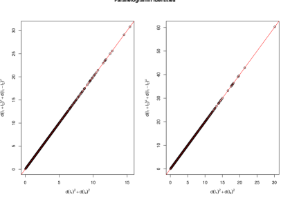
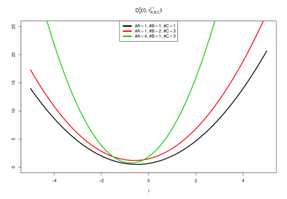
Figure 1: Test of the parallelogramm equality for random lengths $l,l^{\prime}$ and $\#A=\#B=\#C=1$ (above left), $\#A=1,\#B=2,\#C=3$ (above right). On the $x-$axis $\tilde{D}_{2}(0,\tau_{A,B,C}^{l_{1},l_{1}^{\prime}})^{2}+\tilde{D}_{2}(0,\tau_{A,B,C}^{l_{2},l^{\prime}_{2}})^{2}$ is presented. On the $y-$axis $\tilde{D}_{2}(0,\tau_{A,B,C}^{l_{1}+l_{2},l_{1}^{\prime}+l_{2}^{\prime}})^{2}+\tilde{D}_{2}(0,\tau_{A,B,C}^{l_{1}-l_{2},l^{\prime}_{1}-l^{\prime}_{2}})^{2}$ is plotted. Below, the curves $l\mapsto\tilde{D}_{2}(0,\tau_{A,B,C}^{l,1})^{2}$ for different scenarios on $\#A,\#B,\#C$ are plotted.

6 Monotony

For any $X_{0}$-tree $\tau$ let $\tau|_{X}$ denote the restriction to $X\subseteq X_{0}$. Observe that for $\tau\in T_{1}(X_{0})$ in general $\tau|_{X}\notin T_{1}(X)$.

Lemma 12.

Let $X_{0}\supseteq X$ and $\tau,\tau^{\prime}\in T(X_{0})$. Then for $i=1,2,\infty$

$$\begin{array}[c]{*3c}D_{i}(\tau,\tau^{\prime})&\geq&D_{i}(\tau|_{X},\tau^{\prime}|_{X})\\ \tilde{D}_{i}(\tau,\tau^{\prime})&\geq&\tilde{D}_{i}(\tau|_{X},\tau^{\prime}|_{X})\end{array}$$

Proof.

This follows immediately from the same inequalities for semimetrics on $X_{0}$. Then, restricting $d^{*}_{i}\in E(\rho,\rho^{\prime})$ from Lemma 2 to $X\cup X^{\prime}$ yields an element of $E(\rho|_{X},\rho^{\prime}|_{X})$. Moreover,

$$\left\lVert(\delta_{x})_{x\in X_{0}}\right\rVert_{i}\geq\left\lVert(\delta_{x})_{x\in X}\right\rVert_{i}$$

for $\delta\in\mathbb{R}_{\geq 0}^{X_{0}}$ completes the calculation. ∎

Remark 6.

This result naturally holds for many other phylogenetic metrics: for the pathwise difference, NNI-, SPR-, TBR- and maximum parsimony metrics, for example. For the tree rearrangement metrics is was shown in [1, Lemma 2.2].

7 Implementation and numerical examples

The different metrics were implemented by R [35] programs. For solving linear and quadratic programs the glpkAPI library [38] and quadprog library [37] were used, respectively. The corresponding R-script can be downloaded from the website [40]. Some testing showed best performance in terms of computing time for the dual simplex algorithm in the $\ell^{1}$-case. The computing time for obtaining the distance between random trees of size 100 was around 0.3s which is quite reasonable, see Figure 2. It also compares with the computing time of the geodesic distance. The random trees were generated by the function rtree of the R library phangorn [36].

Figure 2: Computing times different metrics (logarithmic scale) for random trees with $n=100$ using the dual simplex algorithm. From left: $D_{1}$ but with primal simplex algorithm, $D_{1}$, $D_{1}$ for $n=200$, $\tilde{D}_{1}$, $D_{2}$, $\tilde{D}_{2}$, the geodesic and the Robinson-Foulds metric.

We also compared $D_{i}$ and $\tilde{D}_{i}$ with several other phylogenetic metrics, essentially the pathwise difference, the geodesic distance and the Robinson-Foulds metric, for $n=10$ leaves. For the computation of the geodesic (BHV-) metric the R-package distory [39] was used. The results are presented in Figure 3. Numerially, we could observe $D_{i}=\tilde{D}_{i}$ in all cases, seee Figure 6 at the end of the paper. A remarkable correlation between the different Gromov-type and the pathwise difference metrics can be observed. There is not much correlation to the geodesic distance. May be, the different weigths on the internal edges (see example 3) are responsible for that.

Similar pictures are found for unweighted trees, see Figure 4. Interestingly, $D_{1}=\tilde{D}_{1}$ turns out to integer-valued now, see the same figure. That is quite a bit surprising since the matrix corresponding to the linear program (8) is not totally unimodular in the sense of [18], it contains the $3\times 3$ submatrix $\begin{pmatrix}1&1&0\\ 1&0&1\\ 0&1&1\end{pmatrix}$ with determinant $-2$.

Random caterpillars are interesting in their own, the results are presented in Figure 5. We observe that we obtain a much larger maximum of 28 for $D_{1}$ (over the sample) than from random trees. In comparison, the lower bound from Lemma 10 would be much smaller: $\frac{n^{2}}{4}-n+2=17$.

Figure 3: Comparison of different metrics for random trees with $n=10$. Above from upper left: $D_{1}$ , $D_{2}$, $D_{\infty}$, $D^{PD}_{1}$, $D_{2}^{PD}$, the geodesic and the Robinson-Foulds metric. Below, the distributions are presented in boxplots.

Figure 4: Comparison of different metrics for random unweighted trees with $n=10$. Above from upper left: $D_{1}$ , $D_{2}$, $D_{\infty}$, $D^{PD}_{1}$, $D_{2}^{PD}$, the geodesic and the Robinson-Foulds metric. In the middle, the distributions are presented in boxplots. At the bottom, the frequency table of $D_{1}$ is presented.

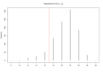
Figure 5: Comparison of different metrics for random caterpillars with $n=10$. Above from upper left: $D_{1}$ , $D_{2}$, $D_{\infty}$, $D^{PD}_{1}$, $D_{2}^{PD}$, the geodesic and the Robinson-Foulds metric. In the middle, the distributions are presented in boxplots. At the bottom, the frequency table of $D_{1}$ is presented with the lower bound from Lemma 10 in red.

8 Discussion

What have we achieved? We constructed at least two new biocomputable metrics for comparing unrooted, but possibly weighted, phylogenetic trees. We think this approach is valuable and could generalise well. One direction is the extension to rooted trees. We should then just measure the distance of the induced metrics on $X\cup\left\{root\right\}$. Another generalisation could be phylogenetic networks. Outside phylogeny, there should be applications to other kinds of finite labeled metric spaces. At the moment, we are only aware of the papers of F.Memoli, e.g. [23], which deals with $\ell^{p}-$type Gromov-Hausdorff metrics.

In general, we follow [31] in arguing that there is no universal metric for phylogenetic trees which suits perfectly for all purposes. We think that every application has its own choice, and we added a further choice to this portfolio. Yet, we should discuss further properties of phylogenetic metrics to guide the users. Monotony as considered in section 6 is a, yet trivial, beginning in this direction. Here we want to discuss some important results of the present paper and possible extensions only.

It looks interesting to extend the metric to tree shapes, with allowing the labels to be permuted. Still that metric differs from the Gromov-Hausdorff metric since we allow only matching of the labels in contrast to the weaker version in (2). For the Gromov-Hausdorff distance it is shown in [25] that it is again NP-hard to compute it. We expect the same for the permutation approach.

One important topic which raised up already in [3, 22, 11, 21] is the question how to weight the edges of the trees. We obtained natural weights from our approach in Example 3. If those weights do not fit the intention of the applicant, it is easy to shorten or lengthen the edges of the trees and obtain other metric spaces which could be easily compared. There is also the possibility to weight the labels, for instance to account for uneven sampling. Then we could adjust to this by weighting the $\left\lVert\cdot\right\rVert_{i}$ norms which leads again to similar computations. Note that we met already such a weighted approach in the computations in the Examples 3 and 4. Further, also a Kantorovich-Wasserstein approach similar to [23] might be feasible if the weights of the leaves differ between the trees. In summary, our approach is natural but can be well adjusted to the needs of applications.

We showed several properties of the new metrics including compatibility with the NNI-metric, a lot of estimates with the pathwise difference metrics, local properties related to the lower bound metrics $\tilde{D}_{i}$, and monotony. Of course, there are many more questions in this context. Especially we would like to sharpen the estimates. We do not know much about the $1-$neighbourhoods on $T_{1}^{2}(X)$, e.g. whether there are islands in the sense of [3]. There are a lot of connections with the quartet, SPR-,TBR-, maximum parsimony, weighted matching and BHV-metrics to explore, too. Numerical comparison was done for the R-implemented distances only.

We expect the diameter between two unweighted $X$-trees to be realised by caterpillar trees. The simulation result in Figure 5 points into this direction. A more sharp estimate than provided in Lemma 9 and Lemma 10 would be quite interesting, too. It is still not clear whether and why $D_{1}$ or $\tilde{D}_{1}$ takes integers values only on $T_{1}^{2}(X)$.

The geometry induced by the euclidean type metrics $D_{2},\tilde{D}_{2}$ should be further explored, too. It should be interesting to prove it is locally euclidean and to find out how the geodesics look like. Possibly, the geodesic distance with respect to $D_{2}$ is even another metric.

Most interesting we find the question whether $D_{i}=\tilde{D}_{i}$. Provable equality could save some computing time, at least. For the time until this problem is solved, we just know there are new animals in the zoo of phylogenetic distances …but not, how many.

Acknowledgements

First of all, I have to thank Mareike Fischer for introducing me to the world of phylogenetic distances. She helped also a lot for getting a clear notation. Second, I’m very grateful to Jürgen Eichhorn who unconsciously draw my attention to metrics between metric spaces. Third, I’d like to thank Michelle Kendall for her inspiring talk at the Portobello conference 2015 and additional discussion later. Fourth, I thank Mike Steel for many interesting discussions, useful hints, his kind hospitality during my stay in Christchurch 2010, and for the organisation of the amazing 2015 workshop in Kaikoura with an inspiring and open atmosphere. Further, Andrew Francis, Alexander Gavryushkin, Stefan Grünewald, Marc Hellmuth and Giulio dalla Riva gave useful hints and inspiration in many discussions.

Appendix A On metric extensions

Several times we met the problem whether a partial dissimilarity on $X$, i.e. a map $q:E\to\mathbb{R}_{\geq 0}$, $E\subseteq\binom{X}{2}$ has an extension to a metric on $X$. This seems to be a well-known problem, one folklore solution I found in [17]:

Theorem 5.

If the graph $G=(X,E)$ is simple and connected then $q:E\to\mathbb{R}_{\geq 0}$ extends to a semimetric on $X$ if and only if for all $x,y\in X$, $\left\{x,y\right\}\in E$, $q(x,y)=d^{q}_{G}(x,y)$.

The graph metric $d^{q}_{G}$ was introduced in (4).

Although this presents a complete solution of the extension problem we want to sharpen this criterion for improved applicability. Still the next result should be folklore but I could not find it in literature. If $p=x_{0}x_{1}\dots x_{m}$ is a cycle in a graph $(X,E)$ we call any pair $\left\{x_{i},x_{j}\right\}\in E$, $0\leq i,j\leq m-1,2\leq\left\lvert i-j\right\rvert\leq m-2$ a chord of $p$. A cycle $p$ without chord is called minimal cycle.

Theorem 6.

If the graph $G=(X,E)$ is simple and connected, then $q:E\to\mathbb{R}_{\geq 0}$ extends to a metric on $X$ if and only if for all minimal cycles $p$ of $G$ and all edges $\left\{x,y\right\}$ in $p$

$$2q(x,y)\leq\mathrm{len}(p).$$ (12)

Proof.

We assume the opposite. Thus we find a (non-minimal) cycle $p=x_{0}x_{1},\dots x_{m}=x_{0}$ such that $e=\left\{x_{0},x_{1}\right\}$ violates (12). We may assume w.l.o.g. that the length of $p$, $m$ is minimal.

Non-minimality of $p$ implies that there is a chord $\left\{x_{i},x_{j}\right\}$ of $p$. Since $m$ is minimal, we know

$$d(x_{i},x_{j})\leq\sum_{k=i}^{j-1}d(x_{k},x_{k+1})$$

and

$$d(x_{0},x_{1})\leq\sum_{k=1}^{i-1}d(x_{k},x_{k+1})+d(x_{i},x_{j})+\sum_{k=j}^{n-1}d(x_{k},x_{k+1})$$

Substituting the first inequality into the RHS of the second one yields

$$d(x_{0},x_{1})\leq\sum_{k=1}^{n-1}d(x_{k},x_{k+1}).$$

This is (12). This contradiction completes the proof. ∎

We can use this result for the

Proof of Theorem 2.

We are using Theorem 6 below on $X\cup X^{\prime}$ with $E=\binom{X}{2}\cup\binom{X^{\prime}}{2}\cup\left\{\left\{x,x^{\prime}\right\}:x\in X\right\}$. The minimal cycles in $(X\cup X^{\prime})$ are either triangles in $X$, triangles in $X^{\prime}$ or rectangles $x,y,y^{\prime},x^{\prime}$. For the two former, (12) is equivalent to the triangle inequalities for $\rho,\rho^{\prime}$. For the latter, (12) is the same as (6). ∎

The following result was used in the proof of Theorem 1.

Lemma 13.

Suppose $X,Y,Z$ are disjoint sets and there are given $d_{1}\in M(X\cup Y)$ and $d_{2}\in M(Y\cup Z)$ such that $d_{1}|_{\binom{Y}{2}}=d_{2}|_{\binom{Y}{2}}$. Then there exists a $d\in M(X\cup Y\cup Z)$ such that $d|_{\binom{X\cup Y}{2}}=d_{1}$ and $d|_{\binom{Y\cup Z}{2}}=d_{2}$.

Proof.

Now we apply the theorem to the graph $(X\cup Y\cup Z,\binom{X\cup Y}{2}\cup\binom{Y\cup Z}{2})$ with $w(u,v)=\left\{\begin{array}[c]{cl}d_{1}(u,v)&u,v\in X\cup Y\\ d_{2}(u,v)&u,v\in Y\cup Z\end{array}\right.$. Since both $X\cup Y$ and $Y\cup Z$ are cliques in this graph, the only minimal cycles are triangles. For them (12) is fulfilled by definition of $w$. ∎

Figure 6: Equality of $D_{i}$ with $\tilde{D}_{i}$, $i=1,2$ for random trees with $n=10$

References

- [1] B. L. Allen and M. Steel, Subtree Transfer Operations and Their Induced Metrics on Evolutionary Trees, Ann. Comb. 5:1–15, 2001
- [2] L.J. Billera, S.P. Holmes, and K. Vogtmann, Geometry of the Space of Phylogenetic Trees, Adv. Appl. Math., 27 (4): 733-767, 2001.
- [3] D. Bogdanowicz and K. Giaro, Matching Split Distance for Unrooted Binary Phylogenetic Trees, IEEE/ACM Transactions on Computational Biology and Bioinformatics 9(1):150-160, 2012
- [4] D. Bogdanowicz, K. Giaro, and B. Wróbel, TreeCmp: Comparison of Trees in Polynomial Time, Evol. Bioinform. Online 8: 475–487, 2012.
- [5] M.L. Bonet and K. St.John. On the complexity of uSPR distance. IEEE/ACM Trans. Comp. Biol. Bioinf. 7(3): 572–-576, 2010
- [6] G.S. Brodal, R. Fagerberg, and C.N.S. Pedersen, Computing the quartet distance between evolutionary trees on time , Proceedings of the 12th International Symposium on Algorithms and Computation (ISAAC). Springer Verlag, Lecture Notes in Computer Science, Vol. 2223, pp. 731–737, 2001
- [7] P. Buneman, The Recovery of Trees from Measures of Dissimilarity. In D.G. Kendall and P. Tautu, eds., Mathematics the the Archeological and Historical Sciences, pages 387–395. Edinburgh University Press, 1971
- [8] P. Buneman, A note on the metric properties of trees, J. Comb. Th., 17(1): 48-50, 1974
-
[9]
J. Cristina, Gromov-Hausdorff convergence of metric spaces, preprint, Helsinki 2008
http://www.helsinki.fi/~cristina/pdfs/gromovHausdorff.pdf - [10] B. DasGupta, X. He, T. Jiang, M. Li, J. Tromp, and L. Zhang, On Distances between Phylogenetic Trees, Proc. Eighth ACM/SIAM Symp. Discrete Algorithms (SODA ’97), pp. 427–436, 1997
- [11] A. Gavryushkin and A. Drummond, The space of ultrametric phylogenetic trees, preprint 2014 arXiv:1410.3544v1
- [12] W.H.E. Day, Optimal algorithms for comparing trees with labeled leaves, J. Class. 2(1):7-28, 1985.
- [13] E. Deza and M.M. Deza, Encyclopedia of Distances, Springer 2009
- [14] A.W.M. Dress, Trees, tight extensions of metric spaces, and the cohomological dimension of certain groups: A note on combinatorial properties of metric spaces, Adv. Math. 53(3): 321-402, 1984
- [15] G. F. Estabrook, F.R. McMorris, and C.A. Meacham, Comparison of Undirected Phylogenetic Trees Based on Subtrees of Four Evolutionary Units, Syst. Zool. 34(2):193-200, 1985
- [16] M. Fischer and S. Kelk, On the Maximum Parsimony distance between phylogenetic trees. In press at Ann. Comb. (preliminary version: Arxiv: 1402.1553)
- [17] A. Guénoche, B. Leclerc, V. Makarenkov, On the extension of a partial metric to a tree metric, Discr. Math. 276: 229-248, 2004.
- [18] A.J. Hoffman, J. Kruskal, Introduction to Integral Boundary Points of Convex Polyhedra, in M. Jünger et al. (eds.), 50 Years of Integer Programming, 1958-2008, Springer Berlin 2010, pp. 49–50
- [19] N. Karmarkar, A new polynomial-time algorithm for linear programming. Combinatorica 4(4): 373–395,1984.
- [20] S. Kelk and M. Fischer, On the complexity of computing MP distance between binary phylogenetic trees, arXiv:1412.4076
- [21] M. Kendall, A new metric for the comparison of phylogenetic trees, talk at the New Zealand phylogenetic conference, Portobello, 2015
- [22] Y. Lin, V. Rajan, and B.M.E. Moret, A metric for phylogenetic trees based on matching, IEEE/ACM Trans. Comp. Biol. Bioinf. 9(4): 1014-1022, 2012
- [23] F. Mémoli, On the Use of Gromov-Hausdorff Distances for Shape Comparison. Symposium on Point Based Graphics 2007, Prague, September 2007.
- [24] M. Owen and J. Provan, A Fast Algorithm for Computing Geodesic Distances in Tree Space, IEEE/ACM Trans. Comp. Biol. Bioinf. 8(1):2 -13, 2011, arXiv:0907.3942
- [25] P.M. Pardalos and H. Wolkowicz(Eds.), Quadratic assignment and related problems, DIMACS Series in Discrete Mathematics and Theoretical Computer Science, 16. American Mathematical Society, Providence, RI, 1994. Papers from the workshop held at Rutgers University, New Brunswick, New Jersey, May 20–21, 1993
- [26] N.D. Pattengale, E.J. Gottlieb, B.M. Moret, Efficiently computing the Robinson-Foulds metric, J. Comput. Biol. 14(6):724-735, 2007.
- [27] D. Penny and M.D. Hendy, The Use of Tree Comparison Metrics, Syst. Biol. 34 (1): 75-82, 1985
- [28] D.F. Robinson, Comparison of Labeled Trees with Valency Three, J. Comb. Th. 11:105-119(1971)
- [29] D.F. Robinson and L.R. Foulds, Comparison of weighted labelled trees, in Combinatorial Mathematics VI, Lecture Notes in Mathematics 748, Springer, Berlin, 1979, pp. 119- 126.
- [30] D.F. Robinson and L.R. Foulds, Comparison of Phylogenetic Trees, Math. Biosciences, 53: 131-147, 1981
- [31] M.A. Steel and D. Penny, Distributions of Tree Comparison Metrics — Some New Results, Syst. Biol.42(2): 126-141, 1993
- [32] C. Whidden, R.G. Beiko, and N. Zeh. Fixed-Parameter and Approximation Algorithms for Maximum Agreement Forests of Multifurcating Trees. To appear in Algorithmica, 2015, arXiv:1305.0512
- [33] W.T. Williams and H.T. Clifford, On the comparison of two classifications of the same set of elements, Taxon 20: 519-522, 1971
- [34] K.A. Zaretskii, Constructing a tree on the basis of a set of distances between the hanging vertices. (in Russian) Uspekhi Mat. Nauk 20(6): 90–92, 1965.
- [35] R Core Team, R: A language and environment for statistical computing, R Foundation for Statistical Computing, Vienna, Austria. URL http://www.R-project.org/, 2015
- [36] K.P. Schliep, phangorn: Phylogenetic analysis in R, Bioinformatics 27(4): 592-593, 2011
- [37] B.A. Turlach (R port by Andreas Weingessel), quadprog: Functions to solve Quadratic Programming Problems, R package version 1.5-5, http://CRAN.R-project.org/package=quadprog, 2013
- [38] G. Gelius-Dietrich, glpkAPI: R Interface to C API of GLPK, R package version 1.3.0, http://CRAN.R-project.org/package=glpkAPI, 2015
- [39] J. Chakerian and S. Holmes, distory: Distance Between Phylogenetic Histories, R package version 1.4.2, http://CRAN.R-project.org/package=distory, 2013
-
[40]
V. Liebscher, R file for figures in the present paper, 2015
http://www.math-inf.uni-greifswald.de/
images/Liebscher/libraries/phylodist.zip