Bubble Universes With Different Gravitational Constants

Abstract

We argue a scenario motivated by the context of string landscape, where our universe is produced by a new vacuum bubble embedded in an old bubble and these bubble universes have not only different cosmological constants, but also their own different gravitational constants. We study these effects on the primordial curvature perturbations. In order to construct a model of varying gravitational constants, we use the Jordan-Brans-Dicke (JBD) theory where different expectation values of scalar fields produce difference of constants. In this system, we investigate the nucleation of bubble universe and dynamics of the wall separating two spacetimes. In particular, the primordial curvature perturbation on superhorizon scales can be affected by the wall trajectory as the boundary effect. We show the effect of gravitational constant in the exterior bubble universe can provide a peak like a bump feature at a large scale in a modulation of power spectrum.

I introduction

In the context of the string theory landscape Susskind:2003kw , there are various possibilities that multiple vacua can be produced whose semiclassical tunnelling process from metastable vacua to new vacua can occur. In this respect, it can allow us to argue that nucleation of spherical symmetric regions, namely Bubble in space which are constructed by a new vacuum and expand into the old vacuum. One of any bubble universe created by such first-order phase transition may be regarded as our universe Basu:1991ig ; Coleman:1980aw ; Sato:1980yn ; Sato:1981gv ; Maeda:1985ye ; Berezin:1987bc ; Bucher:1994gb ; Yamamoto:1995sw ; Garriga:1998he ; Aguirre:2007an ; Simon:2009nb ; Casadio:2011jt ; KeskiVakkuri:1996gn . In particular, inspired by the bubble universe scenario, an accelerated expansion of the universe generated by its vacuum energy would give a natural explanation for inflation realization in the early universe as discussed old inflation Sato:1980yn or open inflation Bucher:1994gb ; Yamamoto:1995sw ; Garriga:1998he scenario in the past. If the bubble universe would be inside the old bubble universe, the so-called parent universe, we are mainly interested in how much information we know or detect through any observational signature of the parent universe.

In the viewpoint of Anthropic principle Susskind:2003kw ; Weinberg:1988cp , it is possible that several universes take their own choices of natural constants. It can allow us to argue a possibility that landscape vacua have different values of gravitational constants as well as cosmological constants. In this paper, the bubble universes have their own different gravitational constants and it can give us explore how a different gravitational constant in the exterior universe affect and relates to physical (especially observational) quantities for the observer in the interior bubble universe (see also works Aguirre:2007an for the aim).

In order to such model building that each bubble universe has its own different gravitational constant, it is useful to employ the JBD theory Brans:1961sx (see book Fujii:2003pa for review). This theory can achieve a varying gravitational constant by identified a vacuum expectation value of the scalar field with gravitational constants in the original, the so-called Jordan frame. Therefore we will use this theory to construct our model and investigate the consequence of the model to our (child) bubble universe, where the child bubble is inside the parent bubble with different constants.

Inflationary scenario can give a remarkably successful way of generating a consistent spectrum of curvature perturbations with recent cosmological observations, such as the cosmic microwave background (CMB) and galaxy survey to explore a large-scale structure Sato:1980yn ; Guth:1980zm ; Lyth-book . The quantum fluctuations generated in a exponential expansion of the early stage of the universe were spread out a cosmological horizon scale and their wavelengths are then pushed to superhorizon size, which can be reduced to classical perturbations seeding cosmic structure. After inflation ends, they reenter the horizon in a radiation dominated phase and can be detected by such as CMB observation (see Lyth-book for review). The recent data by Planck satellite Ade:2013ktc gave a perfectly agreement with the prediction of inflationary theory.

In order to discuss an observational consequence of bubble universes with different gravitational constants, we analyze density perturbations during an inflationary phase based on the JBD theory. Note that although several inflationary models with/without bubble formations and the accompanying density perturbations are discussed based on the scalar-tensor gravity theories including the JBD theory extended_inflation ; soft_inflation ; monopole_inflation , the JBD scalar field is assumed to be an inflaton in those models. In the present paper, however, we assume that there exists an inflaton field in addition to the JBD scalar field, which is used to fix only two different gravitational constants.

If the superhorizon perturbations propagate even though their amplitudes freeze out and approach to the boundary of the bubble universe, they would be scattered by the layer called bubble wall, separating a new and old vacuum. Namely when one join the interior and exterior perturbation mode over the bubble wall, a reflected wave can be produced. Hence if there would be a possibility that one can get information of outside bubble, that is only way to analyze perturbations coming back from superhorizon scales outside bubble as a trace of the outer region (see Ertan:2007eq in a different setup, but in which a similar effect has been studied).

The aim of this paper is to obtain physical signature on a primordial curvature perturbation at superhorizon scales, which is affected by the boundary of bubble. In particular, we can provide how superhorizon mode is modified by the effect of different gravitational constant in the exterior universe by employing the JBD theory.

The paper is organized as follows. In section 2 we show our model setup and discuss a nucleation of bubble universe and a static bubble wall solution. In section 3, we study dynamics of bubble wall after a nucleation. In section 4, we adopt linear perturbation theory to the system and match perturbation modes in both sides over the bubble wall. In particular, our calculation is the case for de Sitter background. Then we discuss the effect of different gravitational constant on the obtained results in section 5. Section 6 is devoted to conclusion.

II model

We consider the model of bubble universes which have their own gravitational constants. The wall of the bubble can divide two bubble universes whose constants have different values. We investigate the effect of different gravitational constant on the superhorizon scale perturbation.

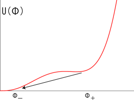
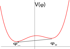
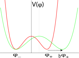
Figure 1: (Left) We plot the potential ${\cal V}(\Phi)$ in the Jordan frame. The tunnelling occurs from $\Phi_{+}$ to $\Phi_{-}$. (Center) We plot the potential $V(\phi)$ in the Einstein frame. The tunnelling occurs from $\phi_{+}$ to $\phi_{-}$. (Right) We plot the symmetric potential (11) and asymmetric one (13). The positive vacuum $\phi_{+}$ where the local minimum is located moves to the right direction by $b$-times with the same height of the potential barrier.

We will introduce the JBD theory Brans:1961sx ; Fujii:2003pa with a potential ${\cal V}(\Phi)$ in the Jordan frame as the model of varying of gravitational constant, which is expressed as the action

$$S=\int d^{4}x\sqrt{-g}\left[{\Phi^{2}\over 2}R-{1\over 2}\partial_{\mu}\Phi\partial^{\mu}\Phi-{\cal V}(\Phi)\right],$$ (1)

where $\Phi$ is the scalar field whose potential is considered to provide their semiclassical tunnelling, namely it has two minima called a true and false vacuum respectively. We use the units of $8\pi G_{N}=1$, where $G_{N}$ is the Newtonian gravitational constant.

From such a potential, the bubble universe will be created as a standard instanton process. The gravitational constant $G$ is related to the vacuum expectation value (VEV) of the scalar field as follows

$$G={G_{N}\over\langle\Phi\rangle^{2}}\,.$$ (2)

The scalar field has a different value depending on each potential minima, and then it can read different values of gravitational constants.

In order to analyze this system, it is useful to study dynamics in the Einstein frame by using conformal transformation as $g_{\mu\nu}=\Phi^{-2}\tilde{g}_{\mu\nu}$maeda1989 . After transformation, the action in the Einstein frame is given by

$$S=\int d^{4}x\sqrt{-\tilde{g}}\left[{\tilde{R}\over 2}-{1\over 2}\partial_{\mu}\phi\partial^{\mu}\phi-V(\phi)\right]\,.$$ (3)

Here we introduced a new scalar field: $\phi$ and its potential, which are related to the original ones in the Jordan frame as

$$\phi=\phi_{0}+\sqrt{7}\ln\Phi,~{}~{}~{}V(\phi)={{\cal V}(\Phi)\over\Phi^{4}}\,,$$ (4)

where $\phi_{0}$ corresponds to the VEV of the JBD scalar field in our universe ($\Phi_{0}=1$). Hereafter we will omit the tilde which represents the variables in the Einstein frame for brevity. In this paper, as expected to generate a bubble, we consider the potential which should give tunnelling, which is expressed by

$$V(\phi)={\lambda\over 8}(\phi^{2}-\mu^{2})^{2}+{\epsilon\over 2\mu}(\phi-\mu)+\Lambda\,.$$ (5)

Under the approximation that $\epsilon$ is small, two vacua are obtained by $\phi_{\pm}=\pm\mu-{\epsilon\over 2\lambda\mu^{3}}+{\cal O}(\epsilon^{2})$ where the suffixes $\pm$ describe two minima. In the case where $\epsilon>0$, the tunnelling occurs from $\phi_{+}$ to $\phi_{-}$ vacuum. Each potential energy is given by $V(\phi_{+})=\Lambda+{\cal O}(\epsilon^{2})$ and $V(\phi_{-})=\Lambda-\epsilon+{\cal O}(\epsilon^{2})$, respectively.

Since we assume that our universe was created by tunnelling from de Sitter universe, our vacuum state is given by $\phi_{0}=\phi_{-}$. From the above potential (5), the potential ${\cal V}(\Phi)$ in the original Jordan frame is found by (4) . In Fig.1, we plot two potentials ${\cal V}(\Phi)$ and $V(\phi)$. From the figure, it is clear that the tunnelling process can be realized from a false($+$) vacuum to a true($-$) vacuum .

II.1 Nucleation of Bubble Universe

We consider a spatially flat Freidmann-Lemaitre-Robertson-Walker (FLRW) spacetime in both sides of the wall. In this case, the instanton process is calculated in the Euclidean spacetime with $O(3)$ symmetry. In the Lorentzian configuration, the line element takes the form

$$ds^{2}=a^{2}(\eta)(-d\eta^{2}+dr^{2}+r^{2}d\Omega^{2})\,,$$ (6)

where $\eta$ is a conformal time which is related to a cosmic time $t$ by $dt=ad\eta$.

Following Basu:1991ig ; KeskiVakkuri:1996gn ; Simon:2009nb , the calculation has been done by use of the complex time path approach, in which dynamics is studied by the complex time $\eta$. By adopting the thin-wall approximation, in which a thickness of wall is small enough compared to the size of a bubble, the bubble radius ${r}(\eta)$ is solved as a function of $\eta$. The action is evaluated as

$$S= \int d\eta\Bigl{[}{4\pi\over 3}\epsilon a^{4}(\eta){r}^{3}(\eta)$$ (7)

$$-4\pi\sigma a^{3}(\eta){r}^{2}(\eta)\sqrt{1-(\partial_{\eta}{r}(\eta))^{2})}\Bigr{]}\,.$$

This action contains both contributions from the volume and surface area of three-dimensional sphere. Here we have used $\epsilon$ and $\sigma$, which are the energy density difference between two vacua and the surface energy density of the wall, respectively. The equation of motion is given by taking a variation of the action $S$ with respect to ${r}$. Solving it, we find a classical trajectory of the wall ${r}(\eta)$. In the backward of time $\eta$, we trace a shrinking bubble radius and reach to a turning point where the canonical momentum ${p}=\partial{\cal L}/\partial(\partial_{\eta}{r})$ vanishes. At this turning point $(\eta=\eta_{i})$, a bubble nucleation occurs. By the analytic continuation, we find the wall trajectory in the complex $\eta$ plane, which shrinks smoothly to zero size of a bubble. In order to perform this procedure, it is useful to rewrite the equation as one for $\eta({r})$. The task to do is reduced to solve it with the boundary conditions:

$${p}=4\pi\sigma{a^{3}{r}^{2}\over\sqrt{(\partial_{{r}}\eta)^{2}-1}}|_{\eta=\eta_{i}}=0\,,~{}~{}~{}\partial_{{r}}\eta(0)=0\,.$$ (8)

where $\eta=\eta_{i}$ denotes a nucleation time.

The tunnelling rate per unit four-volume is obtained from the imaginary part of the action with the complex $\eta$, which becomes

$$\Gamma(\eta_{i})\simeq\exp[-2\,{\rm Im}S(\eta_{i})]\,.$$ (9)

As a result Simon:2009nb , the tunnelling probability in a spatially flat de Sitter universe is obtained as

$${\rm Im}S={\pi^{2}\epsilon\over 3H^{4}}\sinh^{2}\left[{1\over 4}\ln(1+(3H\sigma/\epsilon)^{2})\right]\,.$$ (10)

Note that the tunnelling rate is independent of the choice of $\eta_{i}$ in the de Sitter spacetime. This expression reduces to the result for Minkowski spacetime known as the Coleman’s bubble solution Coleman:1980aw

$${\rm Im}S={27\pi^{2}\sigma^{4}\over 4\epsilon^{3}}\,,$$

in the limit of $H\to 0$.

II.2 Wall solution

We discuss how the difference of the VEV’s $\phi_{\pm}$, that is the difference of gravitational constants in the Jordan frame, affects the observational consequence. So we analyze the dependence of the ratio $G_{+}/G_{-}=\Phi_{-}^{2}/\Phi_{+}^{2}=\exp[-{2\over\sqrt{7}}(\phi_{+}-\phi_{-})]$ on the final result. For simplicity we discuss only the potential in the limit of $\epsilon\to 0$. That is the case of the potential for which both vacua have the same cosmological constant $\Lambda$ .

The potential (5) in this limit is

$$V_{0}(\phi)={\lambda\over 8}\left(\phi^{2}-\mu^{2}\right)^{2}+\Lambda\,.$$ (11)

This gives

$${G_{+}\over G_{-}}=\exp\left[-{4\mu\over\sqrt{7}}\right]\,.$$ (12)

So if we change the value of the parameter $\mu$, we can discuss the dependence of the different gravitational constants. However, it also changes the height of the potential barrier. In order to keep the same potential height, we adopt the following toy potential

$${V}_{0}(\phi)={2\lambda\over(1+b)^{4}}(\phi-b\mu)^{2}(\phi+\mu)^{2}+\Lambda\,.$$ (13)

The values of the scalar field in the mother universe and our universe are given by $\phi_{+}=b\mu$ and $\phi_{-}=-\mu$, respectively. The ratio of the gravitational constants is

$${G_{+}\over G_{-}}=\exp\left[-{2(b+1)\mu\over\sqrt{7}}\right]\,.$$ (14)

Comparing (11) with the case $b\neq 1$ in (13) allows us to discuss the change of the ratio of $G_{+}/G_{-}$ with the same height of the potential barrier (see Fig.1). Calculating the wall solution and surface density of the wall $\sigma$ for this toy potential and varying the value of $b(>-1)$, we can see the effect of the different gravitational constant.

In order to evaluate the surface energy density $\sigma$ of a bubble, we consider a spherical symmetric and static solution $\phi(r)$. The basic equation is

$$\partial_{r}^{2}\phi+{2\over r}\partial_{r}\phi-{dV_{0}\over d\phi}=0\,.$$ (15)

Imposing the thin-wall approximation in which we can neglect the term of $\partial_{r}\phi$, we can integrate it as

$$\int_{\phi_{i}}^{\phi}{d\phi\over\sqrt{2(V_{0}(\phi)-V_{0}(\phi_{i}))}}=r-r_{i}\,,$$ (16)

where $\phi_{i}=\phi(r_{i})$.

For the potential (13), we can find the wall solution as

$${\phi}(r) = -\mu+{(b+1)\mu\over 2}\left[1+\tanh\left({r-r_{i}\over 2d}\right)\right],$$ (17)

with

$$d = {(1+b)\over 2\mu\sqrt{\lambda}}\,.$$ (18)

Of course, in the limit of $b=1$, we find that the solution (17) is reduced to the usual wall solution with the potential (11)

$$\phi(r)=\mu\tanh\Bigl{[}{\mu\sqrt{\lambda}\over 2}(r-r_{i})\Bigr{]}\,.$$ (19)

Then we obtain $\sigma$ as

$$\sigma= \int_{0}^{\infty}dr\left[{1\over 2}(\partial_{r}\phi(r))^{2}+V(\phi)\right]$$

$$\simeq \int_{\phi_{-}}^{\phi_{+}}d\phi\sqrt{2(V_{0}(\phi)-V_{0}(\phi_{-}))}\,,$$ (20)

where we have used the thin-wall approximation. Substituting (13) into the above equation, we obtain the result

$$\sigma(b)={\sqrt{\lambda}\mu^{3}\over 3}(1+b)\,.$$ (21)

When $b=1$, it gives the surface density of the original potential (11) as

$$\sigma|_{b=1}={2\sqrt{\lambda}\over 3}\mu^{3}\,.$$ (22)

We can argue how the difference of gravitational constants in the Jordan frame affects on the bubble nucleation rate $\Gamma$, the wall dynamics and the primordial perturbation through this surface density $\sigma(b)$, which is a function of $b$.

Note that we find the same surface density $\sigma$ even when we take into account of small $\epsilon$-modification of the potential (see Appendix).

III Dynamics of bubble wall

In this section, we study dynamics of a bubble wall after nucleation of a bubble universe. To obtain an analytic solution of a wall trajectory, we assume that a wall is infinitely thin and impose a junction condition across the wall. The bubble dynamics has been studied by several authors Maeda:1985ye ; Berezin:1987bc ; Simon:2009nb ; Casadio:2011jt ; Ertan:2007eq . Following their works, we briefly summarize the results.

Each spacetime is distinguished by the suffixes $+$ and $-$, respectively. The bubble wall is represented as a timelike spherically symmetric hypersurface $\Sigma$ dividing a false ($+$) vacuum and true ($-$) vacuum. We adopt a spatially flat slicing of de Sitter universe for both spacetimes, whose metrics are given by

$$ds_{\pm}^{2}=-dt_{\pm}^{2}+\exp(2H_{\pm}t_{\pm})(dr_{\pm}^{2}+r^{2}_{\pm}d\Omega^{2})\,,$$ (23)

where $H_{\pm}=\sqrt{\Lambda_{\pm}/3}$. Note that

$$H^{2}_{+}-H^{2}_{-}=\epsilon/3\,.$$ (24)

When $\epsilon\neq 0$, cosmological constants inside and outside of the wall have different values. Up to the first order of $\epsilon$, they can be approximated as $\Lambda_{-}=\Lambda-\epsilon$ and $\Lambda_{+}=\Lambda$, respectively. The metric of the bubble wall takes the form

$$ds^{2}|_{\Sigma}=-d\tau^{2}+R^{2}d\Omega^{2}\,.$$ (25)

We assume the stress-energy of this wall is given simply

$$S_{\mu\nu}=-\sigma h_{\mu\nu}\,,$$ (26)

where $h_{\mu\nu}=g_{\mu\nu}-n_{\mu}n_{\nu}$ is the projection tensor on the hypersurface $\Sigma$, which is the metric tensor of (25). The unit spacelike vector $n_{\mu}$ normal to the hypersurface $\Sigma$ is given by

$$n_{\mu}=a\left(-{dr\over d\tau},{dt\over d\tau},0,0\right)\,,~{}n^{\mu}=\left(a{dr\over d\tau},{1\over a}{dt\over d\tau},0,0\right)\,.$$ (27)

From $n^{\mu}n_{\mu}=1$, we obtain the relation equation

$$\left({dt_{\pm}\over d\tau}\right)^{2}-a^{2}_{\pm}\left({dr_{\pm}\over d\tau}\right)^{2}=1\,.$$ (28)

By using ${dr\over d\tau}={dt\over d\tau}\times{dr\over dt}$, it can lead to

$${dt_{\pm}\over d\tau}={1\over\sqrt{1-a_{\pm}^{2}({dr\over dt_{\pm}})^{2}}}\,.$$ (29)

In order to find the dynamical equation for the wall, we use the Israel’s Junction conditions as

$$[g_{\mu\nu}]^{+}_{-}|_{\Sigma}=0\,,$$ (30)

$$[K_{\mu\nu}]^{+}_{-}=-(S_{\mu\nu}-{1\over 2}h_{\mu\nu}S)\,,$$ (31)

where $[X]^{+}_{-}=X|_{+}-X|_{-}$ for the variable $X$ and $S=S^{\mu}_{~{}\mu}$. The extrinsic curvature $K_{\mu\nu}$ of the hypersurface $\Sigma$ is defined by

$$K_{\mu\nu}=h^{\rho}_{\mu}h^{\sigma}_{\nu}\nabla_{\sigma}n_{\rho}\,,$$ (32)

where $\nabla_{\sigma}$ denotes a covariant derivative with respect to $g_{\mu\nu}$. The continuity equation is given as

$$S_{\mu}^{~{}\nu}{}_{||\nu}=-[S^{\rho\sigma}n_{\rho}h_{\mu\sigma}]^{+}_{-}\,,$$ (33)

where $||$ denotes a covariant derivative with respect to the projection tensor $h_{\mu\nu}$. This equation is reduced to the dynamical equation for $\sigma$ as

$${d\sigma(\tau)\over d\tau}=\left[a{dr\over d\tau}{dt\over d\tau}(\rho+P)\right]^{+}_{-}\,,$$ (34)

where $\rho$ and $P$ denote the energy density and pressure in the bulk universes, respectively. If $\rho+P\neq 0$, e.g. for the radiation or matter dominant universe, $\sigma$ changes in time. Throughout this paper, however, since we consider only de Sitter background universes, $\sigma$ turns out to be constant.

From the junction condition (30), we obtain the proper radius of the wall by

$$R=a_{+}r_{+}=a_{-}r_{-}\,.$$ (35)

To find the dynamical equation for $R$, we use the $(\theta\theta)$ component of the second junction equation (31), which leads to

$$K_{\theta\theta}^{+}-K_{\theta\theta}^{-}=-{\sigma\over 2}R^{2}\,,$$ (36)

and its square becomes

$$(K_{\theta\theta}^{+})^{2}={1\over\sigma^{2}R^{4}}\left\{(K_{\theta\theta}^{-})^{2}-(K_{\theta\theta}^{+})^{2}-{\sigma^{2}R^{4}\over 4}\right\}^{2}\,.$$ (37)

While $K_{\theta\theta}$ is calculated as

$$K^{2}_{\theta\theta}=R^{2}\left\{1+\left({dR\over d\tau}\right)^{2}-H^{2}R^{2}\right\}\,.$$ (38)

Using (37), we can simplify the equation for $R$ as

$$\left\{{dR(\tau)\over d\tau}\right\}^{2}=B^{2}R^{2}(\tau)-1\,,$$ (39)

where

$$B^{2} = H^{2}_{+}(1+c_{+}^{2})=H^{2}_{-}(1+c_{-}^{2})\,,$$ (40)

$$c_{\pm} = H^{-1}_{\pm}\left({\epsilon\over 3\sigma}\mp{\sigma\over 4}\right)\,,$$ (41)

where the second equality in (40) is found from Eq. (24). For $c_{+}$, although $\epsilon$ is assumed to be small, $c_{+}$ can be positive because

$${4\epsilon\over 3\sigma^{2}}={12\over(1+b)^{2}}\left({\epsilon\over\lambda\mu^{4}}\right)\left({\mu\over m_{\rm PL}}\right)^{-2}\,,$$ (42)

can be smaller than unity, if we assume $\mu\ll m_{\rm PL}$, where $m_{\rm PL}(=1)$ is the reduced Planck mass.

For de Sitter bulk universes, which we have assumed here, $B$ is a constant and then a solution of a bubble radius $R(\tau)$ is obtained by

$$R(\tau)={1\over B}\cosh B\tau\,.$$ (43)

We can also solve the wall motion in the interior or exterior coordinates $(t_{+},r_{+})$ or $(t_{-},r_{-})$. In what follows, although we give the solution for the exterior coordinates, the same form of the solution is obtained for the interior coordinates just by replacement of $+$ with $-$.

From (35), we have

$$\ln R=H_{+}t_{+}+\ln r_{+}\,,$$ (44)

and differentiate both sides of the equation with respect to $\tau$. Taking its square and using (28) and (43), we find the equation for ${d(\ln r_{+})/d\tau}$ as

$${d(\ln r_{+})\over d\tau}={{\partial_{\tau}(\ln R)}\pm H^{2}_{+}R|c_{+}|\over 1-H^{2}_{+}R^{2}}\,,$$ (45)

which is integrated by using the solution of (43) as

$$r_{+}={r_{\infty+}\cosh B\tau\over|\sinh B\tau\pm c_{+}|}\,,$$ (46)

where $r_{\infty+}$ is an integration constant to be determined later and $\pm$ take $+$($-$), if the sign of $c_{+}$ takes a positive (negative) value. Inserting (46) into (44) leads to the solution of $t_{+}$ as

$$H_{+}t_{+}=\ln(|\sinh B\tau\pm c_{+}|)-\ln Br_{\infty+}\,.$$ (47)

Finally we solve the wall motion as $r_{+}(t_{+})$, which denotes a dynamics of the comoving bubble radius $r$ for the observer in the exterior universe.

Combining ${dR\over d\tau}={dt\over d\tau}\times{d\over dt}(a{r})$, (29) and (43), we have a differential equation

$${-B^{2}R^{2}\over H_{+}}{\partial_{t}{r}(t_{+})\over{r}}=1-|c_{+}|\sqrt{B^{2}R^{2}-1}\,.$$ (48)

It is integrated when rewritten as equation for $B^{2}R^{2}$ as

$${r}_{+}(t_{+})=\sqrt{(a^{-1}_{+}-1)^{2}+c^{-2}_{+}}H^{-1}_{+}\,.$$ (49)

Here we take a nucleation time of a bubble as $t_{+}=0$, when we impose $\partial_{t}{r}_{+}(0)=0$. The solution takes the same form for both interior coordinates too.

We can summarize dynamics of bubble wall in the inside and outside observer as follows. At the initial time $t_{\pm}=0$, the bubble is created at the comoving radii

$${r}_{\pm}(0)={r}_{i\pm}=\left|{\epsilon\over 3\sigma}\mp{\sigma\over 4}\right|^{-1},$$ (50)

and then expands. The comoving radii eventually converge to

$${r}_{\pm}(t\to\infty)=\sqrt{1+c^{2}_{\pm}}{r}_{i\pm}\,\equiv r_{\infty\pm}\,.$$ (51)

The integration constant $r_{\infty+}$ given in (46) should be the same as the above value. The asymptotic comoving radii are rewritten by

$$r_{\infty\pm}=\sqrt{H^{-2}_{\pm}+(r_{i\pm})^{2}}\,.$$ (52)

If we ignore small initial radii $r_{i\pm}$, this equation basically yields $r_{\infty\pm}\sim H^{-1}_{\pm}$, which means the final convergent radii are approximately described by the Hubble radii $H^{-1}_{\pm}$ in each coordinates. It is obviously noted that physical scale of the bubble radius continues to expand as $R=a_{\pm}r_{\pm}\propto e^{H_{\pm}t_{\pm}}$, although the comoving radii converge to about the Hubble radii.

IV Perturbations

In this section, in order to discuss observational effects of the different gravitational constant in the mother universe, we analyze metric perturbations in the Newtonian (longitudinal) gauge. The perturbed metric is given by

$$ds^{2}=a^{2}[-(1+2\psi)d\eta^{2}+(1-2\psi)(dr^{2}+r^{2}d\Omega^{2})]\,.$$ (53)

In the interior and exterior spacetimes, the tunnelling JBD scalar field takes the values of $\phi_{-}$ and $\phi_{+}$, respectively, which provide non-zero cosmological constants. As a result, each bulk universes expand exponentially as de Sitter spacetime. However, such a de Sitter expansion will not end. In order to discuss more realistic cosmological scenario, instead of a cosmological constant, we introduce another scalar field $\varphi$, which is confined at our vacuum state $\phi=\phi_{-}$. This scalar field $\varphi$ is responsible for inflation and will finish the exponential expansion. The quantum fluctuation of this scalar field provides the density perturbations, which we will discuss here .

The new potential $U(\varphi)$ is assumed to be independent of $V(\phi)$. In this case, we find the background equations as

$${\cal H}^{2}={1\over 3}\left({1\over 2}\varphi^{\prime 2}+a^{2}U\right)\,,$$ (54)

$${\cal H}^{\prime}-{\cal H}^{2}=-{1\over 2}\varphi^{\prime 2}\,,$$ (55)

$$\varphi^{\prime\prime}+2{\cal H}\varphi^{\prime}+a^{2}U_{,\varphi}=0\,,$$ (56)

where ${\cal H}=Ha$ and a prime denotes a derivative with respect to a conformal time $\eta$. We assume a slow-roll inflation for $\varphi$ field for simplicity, i.e.

$$a(t)=\exp(Ht),~{}~{}~{}{\cal H}=-{1\over\eta},~{}~{}-{\dot{\varphi}^{2}\over 2}=\dot{H}\,,$$ (57)

where a dot denotes a derivative with respect to the cosmic time $t$. We introduce slow-roll parameters as

$$\varepsilon_{1}=-{\dot{H}\over H^{2}},~{}~{}\varepsilon_{2}={\dot{\varepsilon_{1}}\over H\varepsilon_{1}}\,.$$ (58)

Adding the perturbation of scalar field $\delta\varphi$ and expanding the basic equations up to linear order, we find one master equation by use of the Mukhanov-Sasaki variable $v$, which is a linear combination of $\delta\varphi$ and $\psi$. Defining

$$u={a\psi\over\varphi^{\prime}},~{}~{}~{}v=a\left(\delta\varphi+{\varphi^{\prime}\over H}\psi\right)\,,$$ (59)

we find the basic equations for these variables as

$$\Delta u=z(v/z)^{\prime}\,,~{}~{}v=\theta(u/\theta)^{\prime}\,,$$ (60)

where we have used

$$\theta={{\cal H}\over a\varphi^{\prime}}={1\over a\sqrt{2\varepsilon_{1}}}\,,~{}~{}z={1\over\theta}\,.$$ (61)

Then we obtain the closed master equation for $u$:

$$u^{\prime\prime}-\left(\Delta+{\theta^{\prime\prime}\over\theta}\right)u=0\,.$$ (62)

Under a slow-roll condition, the term $\theta^{\prime\prime}/\theta$ is evaluated as

$${\theta^{\prime\prime}\over\theta}={1\over\eta^{2}}\left(\nu^{2}-{1\over 4}\right)\,,~{}~{}~{}\nu^{2}={1\over 4}+\varepsilon_{1}+{\varepsilon_{2}\over 2}\,.$$ (63)

For spherically symmetric perturbations, a solution $u(r,\eta)=e^{\pm ikr}/r$ satisfies the equation

$$\Delta u=(\partial_{r}^{2}+2\partial_{r}/r)u=-k^{2}u\,.$$

The mode function with a comoving wave number $k$ is obtained by

$$u={e^{\pm ikr}\over r}\sqrt{-\eta}\left[C_{1}H_{\nu}^{(1)}(-k\eta)+C_{2}H_{\nu}^{(2)}(-k\eta)\right]\,,$$ (64)

where $C_{1,2}$ are arbitrary constants. In the interior coordinate($-$) system, $v$ is reduced to $v_{k}\to e^{-ik\eta}/\sqrt{2k}$ in the high-frequency limit, which corresponds to an adiabatic vacuum. This condition fixes the above constants as $C_{1,2}$. Then the solution $u$ is determined up to a phase factor as

$$u_{\rm in}={e^{ik_{-}r_{-}}\over r_{-}}{\sqrt{-\pi\eta_{-}}\over 2k_{-}}H_{\nu}^{(1)}(-k_{-}\eta_{-})\,.$$ (65)

This mode solution is proportional to $e^{ik_{-}(r_{-}-\eta_{-})}$ in the large $|\eta_{-}|$ limit, so interpreted as an incoming wave from the past. It propagates in the outward (large $r_{-}$) direction from inside the bubble and then approaches to the boundary wall.

This incoming wave is scattered at the wall and then divided into reflected and transmitted waves, which are written by

$$u_{\rm rf}={e^{-ik_{-}r_{-}}\over r_{-}}{\sqrt{-\pi\eta_{-}}\over 2k_{-}}H_{\nu}^{(1)}(-k_{-}\eta_{-})\,,$$ (66)

$$u_{\rm tr}={e^{ik_{+}r_{+}}\over r_{+}}{\sqrt{-\pi\eta_{+}}\over 2k_{+}}H_{\nu}^{(1)}(-k_{+}\eta_{+})\,,$$ (67)

respectively. Here the outside wavenumber: $k_{+}$ is related to $k_{-}$ as $k_{+}=(a_{+}/a_{-})k_{-}$ because the phase factor $e^{ik(r\pm\eta)}$ and the proper time $d\tau^{2}=a^{2}_{\pm}(d\eta_{\pm}^{2}-dr^{2}_{\pm})$ have to be invariant across the wall.

The scattered mode $u_{\rm rf}$ is moving in the inward direction and then is going back to the interior bubble. While the mode $u_{\rm tr}$ is transmitted to the outside bubble (the exterior universe).

Expressing each perturbation as

$$u_{-}=u_{\rm in}+\beta u_{\rm rf},~{}~{}~{}u_{+}=\alpha u_{\rm tr}\,,$$ (68)

we match those wave solutions at the hypersurface by use of the junction condition.

The matching has to be done for each proper time of the wall $\tau$. We then impose that the wave amplitudes and their normal derivatives are continuous at the wall hypersurface as

$$u_{-}(\tau)=u_{+}(\tau)\,,$$ (69)

$$n^{\mu}_{-}\partial_{\mu}u_{-}(\tau)=n^{\mu}_{+}\partial_{\mu}u_{+}(\tau)\,.$$ (70)

The similar argument was given in Ertan:2007eq as the matching perturbation across a hypersurface.

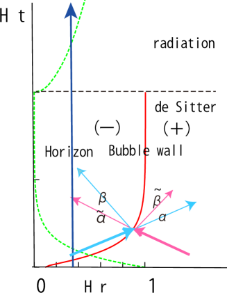
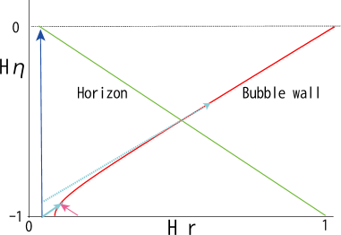
Figure 2: We plot the trajectories representing the bubble wall (red) and horizon scale (green) as seen by a observer outside the wall in the units of $H_{-}=1$. The blue line denotes a typical perturbation scale, which is in superhorizon scale during de Sitter phase. It is shown by the light-blue lines that an incoming wave propagates from inside the bubble to the boundary wall, scattered at the wall and then divided into a reflected $\beta$ and transmitted $\alpha$ waves. The pink line denotes incoming wave from the exterior bubble and scattered into a reflected $\tilde{\beta}$ and transmitted $\tilde{\alpha}$ waves similar as light-blue lines. (Left) We plot them in the coordinate $t$ and comoving radius $r$. (Right) We plot them in the coordinate conformal time $\eta=-1/(aH)$ and comoving radius $r$. It is shown that the slope of incoming wave (light-blue) is an angle of $45^{\circ}$. So at late time, the reflection is not generated since the slope of incoming asymptotically becomes a same slope of the wall trajectory, i.e., $\beta\simeq 0$ and similarly all waves from the exterior bubble can be transmitted, i.e., $\tilde{\alpha}\simeq 1$.

From the wall motion (46) and (47) with (49), the normal vector $n^{\mu}$ (27) is found as

$$n^{t}_{\pm}={|c_{\pm}|\sinh B\tau-1\over\sinh B\tau+|c_{\pm}|}\,,~{}~{}n^{r}_{\pm}={B^{2}r_{\infty\pm}\cosh B\tau\over H_{\pm}(\sinh B\tau+|c_{\pm}|)^{2}}\,.$$ (71)

Rewriting $a_{\pm}$ and $\eta_{\pm}$ as a function of $\tau$ and using the matching conditions (69) and (70), we obtain the amplitudes of the reflected and transmitted waves. We plot some wave trajectory in Fig.2.

In the comoving radial coordinate $r$, the bubble radius (see the red line in Fig.2) increases from an initial value $r_{i}$ to a convergent value $r_{\infty\pm}\simeq 1/H_{\pm}$, while a comoving horizon $1/(H_{\pm}a_{\pm})$ (the green line) decreases monotonically from an initial value $1/H_{\pm}$ where we have set $a_{i}=1$ at an initial time $t=0$ and approaches asymptotically to zero during de Sitter expansion. However if de Sitter expansion continues forever, a typical perturbation mode (as written in a blue line in Fig.2) keeps to be located in superhorizon scale and cannot enter in the horizon again, which is not observable. Such a model does not describe a realistic scenario for cosmological perturbations.

Hence as discussed above, we have added another scalar field $\varphi$, which is responsible for inflation. In a realistic inflationary scenario, inflation will end and lead to reheating of the Universe, connecting to a usual radiation dominated FLRW universe. Taking such a realistic scenario into account, we find the horizon scale increases again from the convergent value, and then such superhorizon perturbation will reenter into the horizon. The initial incoming wave of perturbations approaches to the wall, which is located on over the horizon (see the solid light-blue line with an arrow), and then is scattered into the reflected and transmitted waves. Now we shall analyze how this reflection mode affects the observed quantities, i.e. the CMB power spectrum of the perturbations by the observer lived in the interior bubble universe.

Generally speaking, if one of the bulk spacetimes is not de Sitter, it is difficult to find an analytic solution for the perturbations as well as the background spacetime. We need a complicated numerical analysis. However, since the universe expands exponentially during inflation, we assume the simplest situation for the calculation of the wave propagation, that is, the case of a de Sitter expansion in both sides of spacetime.

In a de Sitter background, we can calculate the reflection amplitude $\beta$ and discuss how this mode affects on perturbations. We match perturbations in both sides at each proper time $\tau$. Eliminating $\alpha$ in the junction conditions (69) and (70), we find $\beta$ as

$$\beta= e^{2ik_{-}r_{-}}\times\Bigl{[}-\Bigl{(}f_{+}(\tau)-f_{-}(\tau)\Bigr{)}H_{\nu}^{(1)}(-k_{+}\eta_{+})H_{\nu}^{(1)}(-k_{-}\eta_{-})$$

$$+g_{+}(\tau)H_{\nu+1}^{(1)}(-k_{+}\eta_{+})H_{\nu}^{(1)}(-k_{-}\eta_{-})-g_{-}(\tau)H_{\nu+1}^{(1)}(-k_{-}\eta_{-})H_{\nu}^{(1)}(-k_{+}\eta_{+})\Bigr{]}$$

$$\times\Bigl{[}\Bigl{(}f_{+}(\tau)-f^{*}_{-}(\tau)\Bigr{)}H_{\nu}^{(1)}(-k_{+}\eta_{+})H_{\nu}^{(1)}(-k_{-}\eta_{-})$$

$$-g_{+}(\tau)H_{\nu+1}^{(1)}(-k_{+}\eta_{+})H_{\nu}^{(1)}(-k_{-}\eta_{-})+g_{-}(\tau)H_{\nu+1}^{(1)}(-k_{-}\eta_{-})H_{\nu}^{(1)}(-k_{+}\eta_{+})\Bigr{]}^{-1}\,,$$ (72)

where $*$ denotes a complex conjugate and

$$f_{\pm}(\tau)=\Bigl{[}(|c_{\pm}|\sinh B\tau-1){H_{\pm}(1+2\nu)\over 2B}+(1-ik_{\pm}r_{\infty\pm}y_{\pm}(\tau)^{-1}\cosh B\tau){B\over H_{\pm}}\Bigr{]}y_{\pm}(\tau)^{-1}\,,$$ (73)

$$g_{\pm}(\tau)=k_{\pm}r_{\infty\pm}(|c_{\pm}|\sinh B\tau-1)y^{-2}_{\pm}(\tau)\,,$$ (74)

$$-k_{\pm}\eta_{\pm}(\tau)={k_{\pm}Br_{\infty\pm}\over H_{\pm}y_{\pm}(\tau)}\,,$$ (75)

with

$$y_{\pm}(\tau)=\sinh B\tau+|c_{\pm}|\,.$$ (76)

We note that in the above calculation we have used the same value of $\nu=1/2$ for the Hankel functions in both sides of the wall. Strictly speaking the order of the Hankel function has to be $\nu_{\pm}$, which depend on the slow-roll parameters $\varepsilon_{1},\varepsilon_{2}$. In our calculation, however, both sides of spacetime are approximated by de Sitter, that is, slow-roll parameters vanish and then we approximate the wave functions with $\nu_{\pm}=\nu=1/2$. We have also used the formula of the Hankel functions: $\partial_{z}H_{\nu}(z)=\nu z^{-1}H_{\nu}(z)-H_{\nu+1}(z)$.

Using the definition of $H_{1/2}(z)$ and $H_{3/2}(z)$, we find

$$\beta=e^{2ik_{-}r_{-}}\times{f_{+}(\tau)-f_{-}(\tau)+{g_{+}(\tau)\over k_{+}\eta_{+}}-{g_{-}(\tau)\over k_{-}\eta_{-}}+i[g_{+}(\tau)-g_{-}(\tau)]\over-(f_{+}(\tau)-f^{*}_{-}(\tau))-{g_{+}(\tau)\over k_{+}\eta_{+}}+{g_{-}(\tau)\over k_{-}\eta_{-}}-i[g_{+}(\tau)-g_{-}(\tau)]}\,.$$ (77)

If $\epsilon$ vanishes exactly, i.e., there is no energy difference between two vacuum states, since $H_{+}=H_{-}$, $f_{+}=f_{-}$, $g_{+}=g_{-}$, and $\eta_{+}=\eta_{-}$, then we find $\beta=0$. However, we assume $\epsilon/3=H_{+}^{2}-H_{-}^{2}\neq 0$, which results in $\beta\propto\epsilon\neq 0$ if $\epsilon$ is small. In fact, assuming $\epsilon\ll\lambda\mu^{4}\times(\mu/m_{\rm PL})^{2}$ as well as $\epsilon\ll\Lambda$, we find

$$\beta = e^{2ik_{-}r_{0}}\times{c_{0}\over\sqrt{1+c_{0}^{2}}\cosh(B_{0}\tau)}{\epsilon\ell^{2}\over 12}\Big{\{}{i\over k_{-}\ell}\left(\sinh(B_{0}\tau)-c_{0}^{-1}\right)$$ (78)

$$+{\sqrt{1+c_{0}^{2}}\over c_{0}}\cosh(B_{0}\tau)\left(1+{\eta_{0}\over\ell}\right)-\sinh(B_{0}\tau)\left(1+{1\over c_{0}^{2}}+{\eta_{0}\over\ell}\right)+{\eta_{0}\over c_{0}\ell}\Big{\}}\,,$$

where we define

$$\ell = \sqrt{3\over\Lambda}=H_{+}^{-1}\,,~{}~{}c_{0}={\ell\sigma\over 4}\,,~{}~{}r_{0}={\ell\sqrt{1+c_{0}^{2}}\over c_{0}}\,,$$

$$B_{0} = {\sqrt{1+c_{0}^{2}}\over\ell}\,,~{}~{}\eta_{0}=-{(1+c_{0}^{2})\ell\over c_{0}(\sinh(B_{0}\tau)+c_{0})}\,.$$ (79)

Similarly, we also have to estimate the contribution from the perturbation in the exterior universe (see the pink line in Fig.2). Now the incoming wave $u$ is given as

$$u_{\rm in}={e^{-ik_{+}r_{+}}\over r_{+}}{\sqrt{-\pi\eta_{+}}\over 2k_{+}}H_{\nu}^{(1)}(-k_{+}\eta_{+})\,.$$ (80)

It is scattered at the wall and then divided into reflected and transmitted waves, which are written by

$$u_{\rm rf}={e^{ik_{+}r_{+}}\over r_{+}}{\sqrt{-\pi\eta_{+}}\over 2k_{+}}H_{\nu}^{(1)}(-k_{+}\eta_{+})\,,$$ (81)

$$u_{\rm tr}={e^{-ik_{-}r_{-}}\over r_{-}}{\sqrt{-\pi\eta_{-}}\over 2k_{-}}H_{\nu}^{(1)}(-k_{-}\eta_{-})\,,$$ (82)

respectively. Expressing each perturbation as

$$u_{+}=u_{\rm in}+\tilde{\beta}u_{\rm rf}\,,~{}~{}~{}u_{-}=\tilde{\alpha}u_{\rm tr}\,,$$ (83)

we match those wave solutions at the hypersurface by use of the junction condition.

Eliminating $\tilde{\beta}$ in the junction conditions (69) and (70), we find the transmitted waves of the perturbations in the exterior universe, that is moving inward direction to the interior universe. The transmitted rate $\tilde{\alpha}$ is given by

$$\tilde{\alpha}={\sqrt{\eta_{+}\over\eta_{-}}}{k_{-}r_{-}\over k_{+}r_{+}}e^{i(k_{-}r_{-}-k_{+}r_{+})}\times\Bigl{[}\Bigl{(}f_{+}(\tau)-f_{+}^{*}(\tau)\Bigr{)}(H_{\nu}^{(1)}(-k_{+}\eta_{+}))^{2}\Bigr{]}$$

$$\times\Bigl{[}\Bigl{(}f_{+}(\tau)-f^{*}_{-}(\tau)\Bigr{)}H_{\nu}^{(1)}(-k_{+}\eta_{+})H_{\nu}^{(1)}(-k_{-}\eta_{-})-g_{+}(\tau)H_{\nu+1}^{(1)}(-k_{+}\eta_{+})H_{\nu}^{(1)}(-k_{-}\eta_{-})$$

$$+g_{-}(\tau)H_{\nu+1}^{(1)}(-k_{-}\eta_{-})H_{\nu}^{(1)}(-k_{+}\eta_{+})\Bigr{]}^{-1}.$$ (84)

Using the definition of $H_{1/2}(z)$ and $H_{3/2}(z)$, we find

$$\tilde{\alpha}=\sqrt{k_{-}\over k_{+}}{H_{-}\over H_{+}}e^{i(k_{-}(r_{-}+\eta_{-})-k_{+}(r_{+}+\eta_{+}))}\times{f_{+}(\tau)-f_{+}^{*}(\tau)\over(f_{+}(\tau)-f^{*}_{-}(\tau))+{g_{+}(\tau)\over k_{+}\eta_{+}}-{g_{-}(\tau)\over k_{-}\eta_{-}}+i[g_{+}(\tau)-g_{-}(\tau)]}\,.$$ (85)

When $\epsilon$ is small, we find

$$\tilde{\alpha}=1+{\epsilon\ell^{2}\over 12}\Biggl{[}2ik_{-}\eta_{0}+{c_{0}\over\sqrt{1+c_{0}^{2}}\cosh(B_{0}\tau)}\Bigg{\{}{i\over k_{-}\ell}\left(\sinh(B_{0}\tau)-c_{0}^{-1}\right)$$

$$-{\sqrt{1+c_{0}^{2}}\over c_{0}}\cosh(B_{0}\tau)\left(4-{1\over c_{0}^{2}}+{2\eta_{0}\over\ell}\right)-\sinh(B_{0}\tau)\left(1+{1\over c_{0}^{2}}+{\eta_{0}\over\ell}\right)+{\eta_{0}\over c_{0}\ell}\Bigg{\}}\Biggr{]}\,.$$ (86)

Once we would obtain the solution of $u$, we have to convert it to the curvature perturbation $\zeta$ and estimate its power spectrum. In Fourier space, we find $\zeta_{k}=v_{k}/z=\theta^{2}(u_{k}/\theta)^{\prime}$.

Hence the curvature perturbation is given by

$$\zeta_{k}= {\sqrt{-\pi\eta_{-}}\over 2k_{-}}e^{-ik_{-}r_{-}}\Biggl{\{}H_{1/2}^{(1)}(-k_{-}\eta_{-})\Bigl{[}{H_{-}\over\sqrt{2\varepsilon_{1-}}}\left({\varepsilon_{2-}\over 2}\beta-{{d\beta\over d\tau}\over{d\eta_{-}\over d\tau}}\eta_{-}\right)+{H_{+}\over\sqrt{2\varepsilon_{1+}}}\left(\left(1+{\varepsilon_{2+}\over 2}-{\eta_{+}\over\eta_{-}}{{d\eta_{-}\over d\tau}\over{d\eta_{+}\over d\tau}}\right)\tilde{\alpha}-{{d\tilde{\alpha}\over d\tau}\over{d\eta_{+}\over d\tau}}\eta_{+}\right)\Bigr{]}$$ (87)

$$-k_{-}\eta_{-}H_{3/2}^{(1)}(-k_{-}\eta_{-})\Bigl{[}{H_{-}\over\sqrt{2\varepsilon_{1-}}}\beta+{H_{+}\over\sqrt{2\varepsilon_{1+}}}{\eta_{+}\over\eta_{-}}{{d\eta_{-}\over d\tau}\over{d\eta_{+}\over d\tau}}\tilde{\alpha}\Bigr{]}\Biggr{\}}\,.$$

Using the definition of Hankel function, a dimensionless power spectrum can be obtained by

$$\Delta_{\zeta}^{2}(k_{-})\equiv{k_{-}^{3}\over 2\pi^{2}}|\zeta_{k}|^{2}$$

$$={1\over 8\pi^{2}}\Bigg{|}(1+ik_{-}\eta_{-}){H_{-}\over\sqrt{\varepsilon_{1-}}}\beta+\left(1+ik_{-}\eta_{-}{\eta_{+}\over\eta_{-}}{{d\eta_{-}\over d\tau}\over{d\eta_{+}\over d\tau}}\right){H_{+}\over\sqrt{\varepsilon_{1+}}}\tilde{\alpha}-{{\eta_{-}}\over{d\eta_{-}\over d\tau}}{H_{-}\over\sqrt{\varepsilon_{1-}}}{d\beta\over d\tau}-{\eta_{+}\over{d\eta_{+}\over d\tau}}{H_{+}\over\sqrt{\varepsilon_{1+}}}{d\tilde{\alpha}\over d\tau}\Bigg{|}^{2}\,,$$ (88)

where we neglected a slow-roll correction, i.e., $\varepsilon_{2\pm}=0$.

We can divide the deviation from the perturbations in a standard inflationary model into three parts $s_{0},s_{1}$ and $s_{2}$, which are of order ${\cal O}(\epsilon)$, as

$$8\pi^{2}\ell^{2}\varepsilon_{1+}\Delta_{\zeta}^{2}(k_{-})\equiv 1+s_{0}+s_{1}+s_{2}+{\cal O}(\epsilon^{2})\,,$$ (89)

with

$$s_{0} = 2{\rm Re}\left(\sqrt{\varepsilon_{1+}\over\varepsilon_{1-}}\beta+(\tilde{\alpha}-1)\right)\,,$$

$$s_{1} = 2{\rm Re}\left(-{{\eta_{-}}\over{d\eta_{-}\over d\tau}}\sqrt{\varepsilon_{1+}\over\varepsilon_{1-}}{d\beta\over d\tau}-{\eta_{+}\over{d\eta_{+}\over d\tau}}{d\tilde{\alpha}\over d\tau}\right)\,,$$

$$s_{2} = 2ik_{-}\eta_{-}\times{\rm Im}\left(\sqrt{\varepsilon_{1+}\over\varepsilon_{1-}}\beta+{\eta_{+}\over\eta_{-}}{{d\eta_{-}\over d\tau}\over{d\eta_{+}\over d\tau}}(\tilde{\alpha}-1)\right)\,.$$ (90)

where Re and Im denote a real and imaginary part, respectively.

At a superhorizon scale ($k_{-}\eta_{-}\ll 1$), the contributions of $s_{0}$ and $s_{1}$ are important, which we can calculate

$$s_{0}={\epsilon\ell^{2}c_{0}\sqrt{\varepsilon_{1+}}\over 6\sqrt{1+c_{0}^{2}}\cosh(B_{0}\tau)}\Biggl{[}-{\sin(2k_{-}r_{0})\over k_{-}\ell\sqrt{\epsilon_{1-}}}\left(\sinh(B_{0}\tau)-c_{0}^{-1}\right)$$

$$+{\sqrt{1+c_{0}^{2}}\over c_{0}}\cosh(B_{0}\tau)\left\{{\cos(2k_{-}r_{0})\over\sqrt{\epsilon_{1-}}}\left(1+{\eta_{0}\over\ell}\right)-{1\over\sqrt{\epsilon_{1+}}}\left(4-{1\over c_{0}^{2}}+{2\eta_{0}\over\ell}\right)\right\}$$

$$-\sinh(B_{0}\tau)\left({\cos(2k_{-}r_{0})\over\sqrt{\epsilon_{1-}}}+{1\over\sqrt{\epsilon_{1+}}}\right)\left(1+{1\over c_{0}^{2}}+{\eta_{0}\over\ell}\right)+{\eta_{0}\over c_{0}\ell}\left({\cos(2k_{-}r_{0})\over\sqrt{\epsilon_{1-}}}+{1\over\sqrt{\epsilon_{1+}}}\right)\Biggr{]}\,,$$ (91)

and

$$s_{1}={\epsilon\ell^{2}c_{0}y_{0}\sqrt{\varepsilon_{1+}}\over 6\sqrt{1+c_{0}^{2}}\cosh(B_{0}\tau)}\Bigg{\{}-{\sin(2k_{-}r_{0})\over k_{-}\ell\sqrt{\varepsilon_{1-}}}{y_{0}\over c_{0}\cosh^{2}(B_{0}\tau)}+\Bigl{(}{\cos(2k_{-}r_{0})\over\sqrt{\varepsilon_{1-}}}+{1\over\sqrt{\varepsilon_{1+}}}\Bigr{)}\times$$

$$\left[-{1\over\cosh^{2}(B_{0}\tau)}\Bigl{(}1+{1\over c_{0}^{2}}+{\eta_{0}\over\ell}\Bigr{)}-{\eta_{0}\over c_{0}y_{0}\ell}\Bigl{(}\cosh(B_{0}\tau)\sqrt{1+c_{0}^{2}}-c_{0}\sinh(B_{0}\tau)+1+{\tanh(B_{0}\tau)y_{0}\over\cosh(B_{0}\tau)}\Bigr{)}\right]$$

$$+{3\eta_{0}\over c_{0}y_{0}\ell}{\cosh(B_{0}\tau)\sqrt{1+c_{0}^{2}}\over\sqrt{\varepsilon_{1+}}}\Biggr{\}}\,,$$ (92)

where

$$y_{0}=\sinh(B_{0}\tau)+c_{0}\,.$$ (93)

The correction $s_{1}$ is derived from the time derivative terms of $\beta$ and $\tilde{\alpha}$, which plays as the order ${\cal O}(1/\cosh(B_{0}\tau))$ and then it can be ignored at the late time, although it can become a leading correction to (91) at the initial time.

At the subhorizon scale ($k_{-}\eta_{-}\mbox{\raisebox{-4.30554pt}{$\stackrel{{\scriptstyle\textstyle>}}{{\textstyle\sim}}$}}1$), the dominant correction term is given by $s_{2}$, which is evaluated by

$$s_{2}=-{\epsilon\ell^{2}k_{-}\eta_{0}\sqrt{\varepsilon_{1+}}\over 6}\Bigg{\{}\Bigl{(}{\cos(2k_{-}r_{0})\over\sqrt{\varepsilon_{1-}}}+{1\over\sqrt{\varepsilon_{1+}}}\Bigr{)}{c_{0}\sinh(B_{0}\tau)-1\over k_{-}\ell\sqrt{1+c_{0}^{2}}\cosh(B_{0}\tau)}-{2k_{-}\eta_{0}\over\sqrt{\varepsilon_{1+}}}$$

$$+{c_{0}\sin(2k_{-}r_{0})\over\sqrt{\varepsilon_{1-}}\sqrt{1+c_{0}^{2}}\cosh(B_{0}\tau)}\left[{\sqrt{1+c_{0}^{2}}\over c_{0}}\cosh(B_{0}\tau)\Bigl{(}1+{\eta_{0}\over\ell}\Bigr{)}-\sinh(B_{0}\tau)\Bigl{(}1+{1\over c_{0}^{2}}+{\eta_{0}\over\ell}\Bigr{)}+{\eta_{0}\over c_{0}\ell}\right]\Biggr{\}}\,.$$ (94)

In order to discuss how those correction terms can be observed, we shall depict them numerically with the specific values of parameters, which we choose

$$\epsilon=10^{-2}\,\ell^{-2},~{}~{}{\rm and}~{}~{}\sigma\geq 0.4\,\ell^{-1}\,.$$ (95)

This inequality guarantees to satisfy the condition $4\epsilon<3\sigma^{2}$ given as (42). In Fig.3, we show a modulation factor of power spectrum ($1+s_{0}+s_{1}+s_{2}$) for different values of $\sigma$. It shows that the modulation factor can be larger in a subhorizon regime: $k_{-}\ell\,\mbox{\raisebox{-4.30554pt}{$\stackrel{{\scriptstyle\textstyle>}}{{\textstyle\sim}}$}}\,1$. For a large value of $c_{0}$, the wall radius has still stayed to be constant. Namely $c_{0}>1$ gives a very tiny modulation, that is a nearly constant amplification in a power spectrum for $\tau=1$. Smaller value of $c_{0}$ shows that the modulation factor is increasing with oscillations in terms of $k$ (e.g. see the plot for $c_{0}=0.3$), which amplitude gets larger for a smaller value of $c_{0}$.

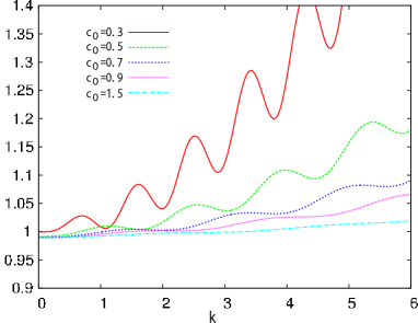
Figure 3: We plot a modulation factor of power spectrum ($1+s_{0}+s_{1}+s_{2}$) given in (89). We set $\epsilon=0.01\ell^{-2}$ and $\tau=\ell$ for each value of $c_{0}=\ell\sigma/4$ and assume slow-roll parameters on both sides of walls are equal as $\sqrt{\varepsilon_{1\pm}}=0.1$.

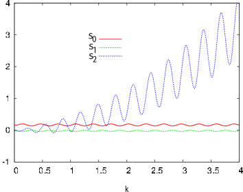
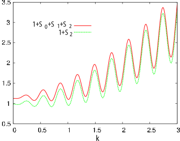
Figure 4: All parameters except for $c_{0}$ are same as used in Fig.3. (Top) We plot three contributions of $s_{0},s_{1}$ and $s_{2}$ for $c_{0}=0.1$. (Bottom) We compare the term $1+s_{2}$ with total one. The term $s_{2}$ can give us a good approximation for describing the total modulation function. The increasing oscillation appears around $k_{-}\ell>1$.

In Fig.4, we plot how each correction contributes to the total modulation of power spectrum. We find that the term $s_{1}$ can be ignored, while $s_{0}$ plays an important role in the superhorizon scale $k_{-}\ell\leq 1$. On the other hand, $s_{2}$ plays an important role in the subhorizon scale, which gives an increasing function of $k$ with oscillations for $k_{-}\ell>1$. This subhorizon effect comes from the one proportional to $(k_{-}\eta_{0})^{2}$ in (94). That is transmitted wave propagating from the exterior universe. Note that the contribution of $s_{2}$ becomes larger than unity, which means a breakdown of perturbative approach for $\epsilon$. The most effective term comes mainly from the one proportional to $(k_{-}\eta_{0})^{2}$ in (94). It gives the condition (96). We can then evaluate a breakdown scale $k_{\rm max}$ of our perturbative treatment for $\epsilon$ as

$${1\over 3}\epsilon\ell^{2}(k_{-}\eta_{0})^{2}<{\cal O}(1)\longrightarrow k_{\rm max}=\sqrt{{3\over\epsilon\ell^{2}}}{c_{0}y_{0}(\tau)\over(1+c_{0}^{2})\ell}\,.$$ (96)

For $c_{0}=0.1$, we find a limited maximum value of wavenumber as $k_{\rm max}\simeq 2.2\ell^{-1}$, beyond which we cannot use this formula.

Of course, these plots also depend on the parameter of the proper time $\tau$ when the waves are scattered. However the plot shows a similar behavior when $\tau<\ell$, although we set $\tau=\ell$ in Fig.3. For $c_{0}=0.1$, the parameter $\tau\,\mbox{\raisebox{-4.30554pt}{$\stackrel{{\scriptstyle\textstyle>}}{{\textstyle\sim}}$}}\,4\ell$ gives no modulation of power spectrum since the wall radius converges to a constant value.

In the observational point of view, the observed power spectrum would be generated by a wave scattered at the wall around which an $e$-folding number takes about $50-60$. If an inflationary period is much longer than $60~{}e$-foldings, it maybe difficult to observe such effect on the CMB power spectrum because the observed modulation is generated at $\tau\gg\ell$ when the wall radius is almost constant. So we have to fine-tune the inflationary model whose period ends around $60~{}e$-foldings. In this case, the value of the modulation is determined by the scattered waves at the wall position when inflation has just started and the radius of the wall is expanding. It will show the deviation from a standard inflationary model.

Note that if the initial radius of the wall is much larger than the horizon scale $H^{-1}=\ell$, i.e., $c_{0}=\sigma\ell/4\ll 1$, we may observe the original perturbation before the scattering at large scale. So there may not appear the modulation for such a larger scale perturbation.

V The effect of Different gravitational constants

In the original Jordan frame, the gravitational constants are different in both vacua, which is given by the VEV’s of the scalar field $\Phi$ by Eq. (2). Since the scalar field $\phi$ is given by Eq. (17), the value changes from $\phi_{-}$ to $\phi_{+}$ suddenly near the bubble wall. Hence the gravitational constants are almost constant both inside and outside of the bubble except near the wall region. The VEV’s in a false($+$) and true($-$) vacua are written by

$$\phi_{+}=b\mu,~{}~{}~{}\phi_{-}(=\phi_{0})=-\mu\,.$$ (97)

Then we find

$$\Phi_{+}=e^{(1+b)\mu/\sqrt{7}},~{}~{}~{}\Phi_{-}=1\,,$$ (98)

which gives

$$G_{+}=e^{-2(1+b)\mu/\sqrt{7}}G_{N},~{}~{}~{}G_{-}=G_{N}\,.$$ (99)

Hence when we analyze the effect of the different gravitational constant in a false vacuum, we should study the dependence of $b$ on our results discussed in the previous section. If one wishes to set almost the same values for both gravitational constants, one needs to choose a negative value of $b$ such that $b\sim-1$, which implies that the value of $\phi$ in a false vacuum is close to that in the true vacuum ($\phi_{+}$). In Fig. 5, we show the gravitational constants for two values of $b$ ($b=1$ and $2$).

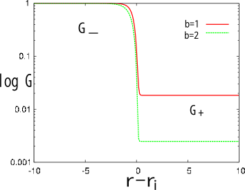
Figure 5: We plot the gravitational constants $G$ for $b=1$ and $b=2$, by setting $\mu=\sqrt{7}$ and $\lambda=1$. We have used the radial coordinate $r$ in the Jordan frame. $r_{i}$ denotes the position of bubble wall.

Since the parameter $b$ is related to the surface density of the wall $\sigma(b)$ as

$$\sigma(b)={\sqrt{\lambda}\mu^{3}\over 3}(1+b)\,,$$ (100)

which is one of the key parameters in our results, we can discuss the effect of the different gravitational constant by changing $\sigma$. In fact, the ratio of two gravitational constants is given by

$${G_{+}\over G_{-}}=\exp\Big{[}-{12\sigma\over\sqrt{7\lambda}\mu^{2}}\Big{]}\,.$$ (101)

Now we study how change of the gravitational constant outside of our universe affects on the final results obtained in the Einstein frame in the previous section. The effects are found mainly in two points; one is the bubble nucleation rate and the other is the power spectrum of curvature perturbations, which we shall discuss in due order.

V.1 Nucleation rate of the bubble with
different gravitational constant

The bubble nucleation rate is given by (9) and (10), which is described as

$$\Gamma\simeq\exp\Bigl{[}-{\pi^{2}\sigma\over 2H^{3}}\Bigr{]}\,,$$ (102)

in the limit qof $\epsilon\rightarrow 0$. This result shows that the larger value of $\sigma$ makes tunnelling process suppressed highly by a huge exponential factor. If $\sigma\simeq 0$, i.e., $b\simeq-1$, which means the difference of gravitational constants is very small, the nucleation probability becomes very high. This is easily understood as follows: By assuming that $\mu$ and $\lambda$ are fixed, when the value of $b$ changes from $-1$ to $\infty$, the surface tension $\sigma$ takes the value from $0$ to $\infty$. It is because the wall barrier height is constant but the width becomes narrower as $b$ decreases. When we change the gravitational constant in a false vacuum, however, if we fix $\sigma$, i.e., the potential is given by the relation such that

$$\lambda\mu^{4}(\phi_{+}-\phi_{-})^{2}\,,$$ (103)

is constant, the nucleation probability does not change. Hence whether the universe with a different gravitational constant is plausible or not depends on the choice of the potential form.

V.2 Curvature perturbations

The power spectrum of curvature perturbations which reenter inside the horizon of our bubble universe is evaluated by considering both reflected $\beta$ and transmitted $\tilde{\alpha}$ waves. The modulation factor of a normalised power spectrum of curvature perturbations (89)-(94) is affected by changing $\sigma(b)$. In what follows, we assume $\mu=\sqrt{7}$ just for simplicity, and then compare the case of $b=1$ with that of $b=2$. If the surface density takes the value $\sigma=0.4\ell^{-1}$ for $b=1$, we find $\sigma=0.6\ell^{-1}$ for $b=2$. The gravitational constant $G_{+}$ for $b=2$ of the exterior of the bubble takes smaller value than the case of $b=1$ by the factor $e^{-2}\simeq 0.1$ because $(1+b)$ becomes three halves (see Fig.5).

For small value of $\epsilon$, which we assume through this paper, which have been obtained as (91)-(94), we plot the effect of difference of gravitational constants on the power spectrum in Fig.6. The modulation factor ($1+s_{0}+s_{1}+s_{2}$), which describes a correction from a standard scale-invariant spectrum, shows oscillatory bumps at a small scale $k_{-}\,\mbox{\raisebox{-4.30554pt}{$\stackrel{{\scriptstyle\textstyle>}}{{\textstyle\sim}}$}}\,1/\ell$ and its amplitude increases for smaller $k_{-}$. It also increases for a smaller value of the parameter $\sigma$. By using (94), the term such as $\cos(2k_{-}r_{0})$ gives the oscillation period $\Delta k\simeq\pi/r_{0}\propto\sigma$ for small $\sigma$. Therefore when $b$ becomes a half, the period $\Delta k$ becomes more sharp by twice.

We conclude the effect of different gravitational constant on the final power spectrum as follows. The typical signature appears on a small scale and it gives an increasing oscillation. Especially, if the gravitational constants for both sides of the wall is close to each other, i.e., $\sigma\approx 0$ ($b\approx-1$), the modulation of power spectrum becomes larger. The feature where an increasing oscillation appears on small scale is generated by the transmitted $\tilde{\alpha}$ wave of perturbation in the exterior bubble universe (see (86)), and can be constrained by the observation of CMB.

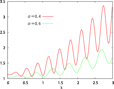
Figure 6: We plot the final power spectrums for $\sigma=0.4\ell^{-1}$ and $\sigma=0.6\ell^{-1}$.

VI Concluding remarks

We have argued a possible scenario that each universe takes its own different value of gravitational constant in the context of the emergence of the bubble universes. In order to construct a model that makes different gravitational constants corresponding to several vacua, we adopt the JBD theory, with which taking different values of the VEV of the JBD scalar field, the universes with different gravitational constants are achieved. In particular, we investigate the effect of different gravitational constant in the exterior universe on primordial curvature perturbations observed in the interior bubble universe.

Via a conformal transformation, we can simply analyze the physics in the Einstein frame, that is the nucleation of bubbles, the evolution of bubble wall and matching curvature perturbations of the interior and exterior region. In the Jordan frame, it becomes clear that the final power spectrum of curvature perturbation is affected by the bubble boundary through the surface energy density $\sigma$ of the wall. The key parameter is $b$, which is $b=\phi_{+}/|\phi_{-}|$, where $\phi_{\pm}$ is the VEV’s of the JBD scalar field in the interior and exterior universes. The parameter $b$ is related to the ratio of gravitational constants as $-2(b+1)\mu/\sqrt{7}=\log(G_{+}/G_{-})$. In Fig. 3, for different values of $\sigma$, we show the modulation of the power spectrum, which has several peaks with growing oscillation in Fourier space. If the gravitational constant in the exterior universe gets smaller, $b$ or $\sigma$ increases and then the modulation becomes smaller. Choosing a smaller parameter $\sigma$ will heighten the amplitude of peak shown in the modulation of power spectrum of curvature perturbations.

In our result, we assume that the $e$-foldings of inflationary period is about $60$, because the initial modulation of perturbations will not be observed for inflationary models with the $e$-foldings more than $60$. In this paper, we have not discussed after inflation. The result obtained from perturbations matching at later time such as a radiation dominated era will be more interesting and important, although it is difficult to describe a trajectory of the bubble wall in an analytic form. In order to solve dynamics of wall in this phase, we may need numerical treatment. Along this direction, we hope to make a progress in our future work.

Appendix A domain wall solution and surface energy for small $\epsilon$

We consider the following potential

$$V = V_{0}+\epsilon V_{1}$$ (104)

$$= {2\lambda\over(b+1)^{4}}(\phi-b\mu)^{2}(\phi+\mu)^{2}$$

$$+{\epsilon\over(b+1)\mu}(\phi-b\mu)+\Lambda\,.$$

There are three extrema

$$\phi_{+} = b\mu-\epsilon{(b+1)\over 4\lambda\mu^{3}}\,,$$ (105)

$$\phi_{B} = {b-1\over 2}\mu+\epsilon{(b+1)\over 2\lambda\mu^{3}}\,,$$ (106)

$$\phi_{-} = -\mu-\epsilon{(b+1)\over 4\lambda\mu^{3}}\,.$$ (107)

$\phi_{+}$ and $\phi_{-}$ correspond to the local minima, while $\phi_{B}$ is the local maximum, at which the potential values are by given

$$V(\phi_{+}) = \Lambda+O(\epsilon^{2})\,,$$ (108)

$$V(\phi_{B}) = \Lambda+{\lambda\over 8}\mu^{4}-{\epsilon\over 2}+O(\epsilon^{2})\,,$$ (109)

$$V(\phi_{-}) = \Lambda-\epsilon+O(\epsilon^{2})\,.$$ (110)

Although $\phi_{+}$ can be shifted by changing a free parameter $b$, the potential barrier and the minimum values do not depend on $b$.

Now we find a domain wall solution for this potential $V$. Plugging $\phi=\phi_{0}(r)+\epsilon\phi_{1}(r)$ into the basic equation and expanding it up to the first order of small parameter $\epsilon$, we find the following equations:

$$\phi_{0}^{\prime\prime}+{1\over r}\phi_{0}^{\prime}-{dV_{0}\over d\phi}(\phi_{0})=0\,,$$ (111)

$$\phi_{1}^{\prime\prime}+{1\over r}\phi_{1}^{\prime}-{d^{2}V_{0}\over d\phi^{2}}(\phi_{0})\phi_{1}-{1\over(b+1)\mu}=0\,.$$ (112)

By using thin wall approximation, Eq. (111) gives the 0-th order domain wall solution as

$$\phi_{0}={(b-1)\over 2}\mu+{(b+1)\over 2}\mu\tanh\left({r-r_{i}\over 2d}\right)\,.$$ (113)

Using this solution, we find

$${d^{2}V_{0}\over d\phi^{2}}(\phi_{0})={4\lambda\mu^{2}\over(b+1)^{2}}\left[1-{3\over 2\cosh^{2}\left({r-r_{i}\over 2d}\right)}\right]\,.$$ (114)

If we ignore the deviation form unity near $r=r_{i}$ this term can be treated as a constant. Then we find an approximate solution for $\phi_{1}$ as

$$\phi_{1}=-{(b+1)\over 4\lambda\mu^{3}}\left[1-{D\over d\cosh^{2}\left({r-r_{i}\over 2d}\right)}\right]\,,$$ (115)

where $D$ is an arbitrary constant.

This solution $\phi=\phi_{0}+\epsilon\phi_{1}$ can be rewritten as

$$\phi = {(b-1)\over 2}\mu-\epsilon{(b+1)\over 4\lambda\mu^{3}}$$ (116)

$$+{(b+1)\over 2}\mu\tanh\left({r-r_{i}+\delta r_{\epsilon}\over 2d}\right)\,,$$

where $\delta r_{\epsilon}={\epsilon\over\lambda\mu^{4}}D$. This domain wall solution is just shifted from one with $\epsilon=0$ by $-\epsilon{(b+1)\over 4\lambda\mu^{3}}$ and $-\delta r_{\epsilon}$ in $\phi$- and $r$-directions, respectively. The domain wall structure itself does not change.

Next we shall calculate the surface energy density, which is defined by

$$\sigma = \int_{0}^{\infty}dr\left[{1\over 2}(\partial_{r}\phi)^{2}+V_{\rm DW}(\phi)\right]\,,$$ (117)

where $V_{\rm DW}$ is the part of the potential which contributes to the structure of a domain wall.

Plugging the above solution (116) into the kinetic term and potential, we find up to the first order of $\epsilon$ as

$${1\over 2}(\partial_{r}\phi)^{2} = {\lambda\mu^{4}\over 8\cosh^{4}\left({r-r_{i}+\delta r_{\epsilon}\over 2d}\right)}\,,$$ (118)

$$V(\phi) \approx {\lambda\mu^{4}\over 8\cosh^{4}\left({r-r_{i}+\delta r_{\epsilon}\over 2d}\right)}+{\epsilon\tanh\left({r-r_{i}\over 2d}\right)\over 4\cosh^{2}\left({r-r_{i}\over 2d}\right)}$$ (119)

$$+ {\epsilon\over 2}\left[\tanh\left({r-r_{i}\over 2d}\right)-1\right]+\Lambda\,.~{}~{}~{}~{}$$

The potential $V$ contains a back ground bulk energy, i.e., cosmological constants;

$$V_{\rm bulk}=\Lambda-{\epsilon\over 2}\left[1-{\rm sgn}(r-r_{i})\right]\,.$$ (120)

where the sign function ${\rm sgn}(x)$ is defined by

$${\rm sgn}(x)=\left\{\begin{array}[]{ccc}1&{\rm if}&x>0\\ -1&{\rm if}&x<0\\ \end{array}\right.\,.$$ (123)

Since the bulk energy should not be included in the surface energy of the wall, we define

$$V_{\rm DW} := V(\phi)-V_{\rm bulk}$$ (124)

$$= {\lambda\mu^{4}\over 8\cosh^{4}\left({r-r_{i}+\delta r_{\epsilon}\over 2d}\right)}+{\epsilon\tanh\left({r-r_{i}\over 2d}\right)\over 4\cosh^{2}\left({r-r_{i}\over 2d}\right)}$$

$$+{\epsilon\over 2}\left[\tanh\left({r-r_{i}\over 2d}\right)-{\rm sgn}(r-r_{i})\right]\,.$$

In the thin-wall approximation ($d\ll r_{i}$), the surface energy $\sigma$ is evaluated approximately as

$$\sigma \approx \int_{-\infty}^{\infty}dr\left[{1\over 2}(\partial_{r}\phi)^{2}+V_{\rm DW}(\phi)\right]$$ (125)

$$= {\lambda\mu^{4}\over 4}\int_{-\infty}^{\infty}{dr\over\cosh^{4}\left({r-r_{i}+\delta r_{\epsilon}\over 2d}\right)}\,,$$

which gives the same result as the case with $\epsilon=0$, i.e.,

$$\sigma\approx{\sqrt{\lambda}\mu^{3}(b+1)\over 3}\,.$$ (126)

It is plausible because the domain wall structure does not change by the small $\epsilon$-modification of the potential.

References

- (1) L. Susskind, In Universe or multiverse? ed by B. Carr, pp247-266, hep-th/0302219.
- (2) S. R. Coleman and F. De Luccia, Phys. Rev. D 21, 3305 (1980).
- (3) K. Sato, Mon. Not. Roy. Astron. Soc. 195 467 (1981).
- (4) K. Sato, H. Kodama, M. Sasaki and K. Maeda, Phys. Lett. B 108, 103 (1982); K. Maeda, K. Sato, M. Sasaki, H. Kodama Phys.Lett. B 108, 98 (1982).
- (5) K. Maeda, Gen. Rel. Grav. 18, 931 (1986).
- (6) V. A. Berezin, V. A. Kuzmin and I. I. Tkachev, Phys. Rev. D 36, 2919 (1987).
- (7) R. Basu, A. H. Guth and A. Vilenkin, Phys. Rev. D 44, 340 (1991).
- (8) M. Bucher, A. S. Goldhaber and N. Turok, Phys. Rev. D 52, 3314 (1995), hep-ph/9411206.
- (9) K. Yamamoto, M. Sasaki and T. Tanaka, Astrophys. J. 455, 412 (1995), astro-ph/9501109.
- (10) E. Keski-Vakkuri and P. Kraus, Phys. Rev. D 54, 7407 (1996), hep-th/9604151.
- (11) J. Garriga, X. Montes, M. Sasaki and T. Tanaka, Nucl. Phys. B 551, 317 (1999), astro-ph/9811257.
- (12) A. Aguirre, M. C. Johnson and A. Shomer, Phys. Rev. D 76, 063509 (2007), arXiv:0704.3473.
- (13) D. Simon, J. Adamek, A. Rakic and J. C. Niemeyer, JCAP 0911, 008 (2009), arXiv:0908.2757.
- (14) R. Casadio and A. Orlandi, Phys. Rev. D 84, 024006 (2011), arXiv:1105.5497.
- (15) S. Weinberg, Rev. Mod. Phys. 61, 1 (1989).
- (16) P. Jordan, Zeil. Phys. 157, 112 (1959); C. Brans and R. H. Dicke, Phys. Rev. 124, 925 (1961).
- (17) Y. Fujii and K. Maeda, The scalar-tensor theory of gravitation, (Cambridge. Univ. Press, 2003).
- (18) D. La and P. J. Steinhardt, Phya. Rev. Lett. 62, 376 (1989); Phys. Lett. B 220, 375 (1989); D. La, P. J. Steinhardt, and E. Bertschinger, Phys. Lett. B 231, 231 (1989).
- (19) A.L. Berkin, K. Maeda, J. Yokoyama, Phys. Rev. Lett. 65, 141 (1990); A.L. Berkin, K. Maeda, Phys.Rev. D44, 1691 (1991).
- (20) N. Sakai, J. Yokoyama, K. Maeda, Phys.Rev. D59, 103504 (1999), gr-qc/9811024.
- (21) A. H. Guth, Phys. Rev. D23 347 (1981).
- (22) D. H. Lyth and A. Liddle, Cosmological inflation and large-scale structure, (Cambridge Univ. Press, 2009).
- (23) P. A. R. Ade et al. [Planck Collaboration], Astron. Astrophys. 571, A1 (2014), arXiv:1303.5062; P. A. R. Ade et al. [Planck Collaboration], Astron. Astrophys. 571, A22 (2014), arXiv:1303.5082.
- (24) E. Ertan and A. Kaya, Gen. Rel. Grav. 40, 1511 (2008), arXiv:0704.2284.
- (25) K. Maeda, Phys.Rev. D39 3159 (1989).
- (26) K. Maeda, Phys.Lett. B186, 33 (1987).
- (27) J. Martin and R. H. Brandenberger, Phys. Rev. D63, 123501 (2001), hep-th/0005209; R. H. Brandenberger and J. Martin, Class. Quant. Grav. 30, 113001 (2013), arXiv:1211.6753.
- (28) U. H. Danielsson, Phys. Rev. D66, 023511 (2002), hep-th/0203198.
- (29) R. Easther, B. R. Greene, W. H. Kinney and G. Shiu, Phys. Rev. D66, 023518 (2002), hep-th/0204129.