T-MATRIX IN DISCRETE
OSCILLATOR REPRESENTATION

Abstract

We investigate T-matrix for bound and continuous-spectrum states in the discrete oscillator representation.  The investigation is carried out for a model problem – the particle in the field of a central potential.  A system of linear equations is derived to determine the coefficients of the T-matrix expansion in the oscillator functions.  We selected four potentials (Gaussian, exponential, Yukawa, and square-well ones) to demonstrate peculiarities of the T-matrix and its dependence on the potential shape.  We also study how the T-matrix expansion coefficients depend on the parameters of the oscillator basis such as the oscillator length and the number of basis functions involved in calculations.

1 Introduction

We are going to consider the convergence of a wave function and the T-matrix expansion in the oscillator functions.  This consideration will be restricted to a model problem of the particle in the field of a central potential.  The analysis will be done within the matrix form of quantum mechanics, which involves an infinite set of oscillator functions to realize a discrete representation.  This matrix form is well known as the algebraic version of the resonating group method or J-matrix method.  The methods were formulated in [1,​ 2] and [3,​ 4], respectively.  Now, they are widely used to describe nuclear, atomic, and molecular systems.  In Ref. [5], one can find progress in resolving the internal problems of the method and the numerous applications to solving real physical problems in different branches of quantum physics.

Usually, the expansion of a wave function in the oscillator or any other square-integrable basis is considered within the J-matrix.  The discrete form of the T-matrix has not been investigated yet.  For instance, in Ref. [6], the oscillator basis was used to construct wave functions and to calculate the phase shift for a Gaussian potential.  The T-matrix was also obtained in that paper, but only in the momentum space.  So, we are going to fill in this gap.  We consider the states of both discrete and continuous spectra.  However, the main attention will be paid to the scattering states.

We are going to demonstrate the convergence of the T-matrix and how the convergence depends on the shape of a potential, on the oscillator length of a basis and the energy of the state.  For this aim, we selected four potentials, which mimic different physical systems.  Note that, by solving model problems, one can reveal the interesting features and peculiarities of systems under consideration, which are observed in more complicated and realistic systems.  For instance, it was discovered in Refs. [7,​ 8], while studying simple model problems, that the J-matrix in some cases suffers of a slow convergence.  This means that one needs to involve a very large basis of oscillator functions to achieve the desired precision of calculations.  An effective method was formulated in [8,​ 9,​ 10].  It allows one to reduce the set of oscillator functions by three-five times in order to obtain the phase shifts with higher precision.

The paper is organized in the following way.  In Section 2, we make all necessary definitions and deduce the equations for the T-matrix expansion coefficients.  We briefly consider main equations, which are used to describe quantum systems.  These equations will be transformed from a continuous (coordinate or momentum) representation to a discrete, oscillator representation.  The analysis of the T-matrix in the discrete representation is presented in Section 3 for four potentials (Gaussian, Yukawa, exponential, and square-well ones).

2 Model Formulation

We make use of the system of units by selecting the constant $\hbar^{2}/m=1$.  This leads to a renormalization of the potential energy operator

$$\widehat{V}\left(r\right)\Rightarrow\frac{m}{\hbar^{2}}\widehat{V}\left(r\right)\!.$$

In this representation, the kinetic energy operator is $\widehat{T}=-\frac{1}{2}\mathbf{\nabla}^{2}$ in coordinate space and $\widehat{T}=\frac{1}{2}\mathbf{p}^{2}$ in the momentum space, and the energy is $E=\frac{1}{2}k^{2}$.  In this paper, we will consider central potentials.  Thus, the orbital momentum $L$ is a good quantum number.

2.1 Basic equations

To determine the spectrum of bound states and their wave functions or to determine the scattering parameters and the corresponding functions for continuous spectrum states, one should solve the Schrödinger equation

$$(\widehat{H}-E)\Psi_{kL}\left(r\right)=0$$ (1)

or the Lippmann–Schwinger equation

$$\Psi_{kL}\left(x\right)=\psi_{kL}\left(x\right)-$$

$$-\int G\left(x,\widetilde{x}\right)\widehat{V}\left(\!\widetilde{x},\widetilde{\widetilde{x}}\right)\Psi_{kL}\left(\widetilde{\widetilde{x}}\right)\ \widetilde{x}^{2}d\widetilde{x}\widetilde{\widetilde{x}}^{2}d\widetilde{\widetilde{x}}.$$ (2)

The latter can be written in the coordinate space ($x=r$) or in the momentum space ($x=p$).  In the coordinate space, we have

$$\psi_{kL}\left(r\right)=\sqrt{\frac{2}{\pi}}kj_{L}\left(kr\right)\!,$$ (3)

$$G\left(r,\widetilde{r}\right)=j_{L}\left(kr_{<}\right)n_{L}\left(kr_{>}\right)\!,$$ (4)

$$\widehat{V}\left(\widetilde{x},\widetilde{\widetilde{x}}\right)=\delta\left(\widetilde{r}-\widetilde{\widetilde{r}}\right)\widehat{V}\left(\widetilde{r}\right)$$ (5)

($r_{<}=\min\left(r,\widetilde{r}\right),\ r_{>}=\max\left(r,\widetilde{r}\right)$) and in the momentum space

$$\psi_{kL}\left(p\right)=\delta\left(p-k\right),$$ (6)

$$G\left(p,\widetilde{p}\right)=\left(\!\frac{1}{2}p^{2}-\frac{1}{2}k^{2}+i\varepsilon\!\right)^{\!\!-1}\!\delta\left(p-\widetilde{p}\right)\!,$$ (7)

$$\widehat{V}\left(p,\widetilde{p}\right)=\frac{2}{\pi}p\widetilde{p}\int\limits_{0}^{\infty}j_{L}\left(pr\right)\widehat{V}\left(r\right)j_{L}\left(\widetilde{p}r\right)r^{2}dr.$$ (8)

Note that the transition from the coordinate space to the momentum one is determined by the Fourier–Bessel integral

$$\Psi_{kL}\left(p\right)=\sqrt{\frac{2}{\pi}}p\int\limits_{0}^{\infty}j_{L}\left(pr\right)\Psi_{kL}\left(x\right)r^{2}dr.$$ (9)

There is another equation, which is also used to determine the spectrum and the wave functions of bound and scattering states.  This is the Lippmann–Schwinger equation for the half-off shell transition T-matrix (see, e.g., [11,​ 12])

$$t_{L}\left(p,k\right)=V_{L}\left(p,k\right)+\int\limits_{0}^{\infty}d\widetilde{p}\widetilde{p}^{\,2}\frac{V_{L}\left(p,\widetilde{p}\right)t_{L}\left(\widetilde{p},k\right)}{E-\frac{1}{2}\widetilde{p}^{2}+i\epsilon}.$$ (10)

There are several equivalent definitions of the T-matrix, in particular, those, which involve integrals with the potential energy operator and the wave function

$$t_{L}\left(p,k\right)=\sqrt{\frac{2}{\pi}}p\int\limits_{0}^{\infty}drr^{2}j_{L}\left(pr\right)\widehat{V}\left(r\right)\Psi_{kL}\left(r\right)$$ (11)

in the coordinate space or, in the momentum space,

$$t_{L}\left(p,k\right)=\int\limits_{0}^{\infty}d\widetilde{p}\widetilde{p}^{2}\widehat{V}\left(p,\widetilde{p}\right)\Psi_{kL}\left(\widetilde{p}\right)\!.$$ (12)

We present the following important relation, which connects the T-matrix and the wave function in the momentum space:

$$\Psi_{kL}\left(p\right)=\delta\left(p-k\right)-\frac{t_{L}\left(p,k\right)}{\frac{1}{2}p^{2}-\frac{1}{2}k^{2}}.$$ (13)

By calculating the T-matrix, we can easily construct the wave function of a system in the momentum space.

It is well known that, in order to determine the spectrum and wave functions by solving the Schrödinger equation, one needs to impose the adequate boundary conditions, while the necessary boundary conditions are included in the Lippmann–Schwinger equation.

In the present paper, we use the standing-wave representation, which means that the asymptotic part of wave functions is

$$\Psi_{kL}^{\left(a\right)}\left(r\right)=\sqrt{\frac{2}{\pi}}k\ j_{L}\left(kr\right)-\tan\delta_{L}\sqrt{\frac{2}{\pi}}k\ n_{L}\left(kr\right)\!,$$

where $\delta_{L}$ is the phase shift, and $\ j_{L}\left(kr\right)$ and $\ n_{L}\left(kr\right)$ are Bessel and Neumann functions, respectively.  However, the T-matrix is usually determined with the wave function in the running-wave representation. In this representation,

$$\Psi_{kL}^{\left(a\right)}\left(r\right)=\ \left[\psi_{L}^{\left(-\right)}\left(kr\right)-S_{L}\psi_{L}^{\left(+\right)}\left(kr\right)\right]\!\!.$$

Here, $S_{L}=\exp\left\{2i\delta_{L}\right\}$ is the scattering matrix, and

$$\psi_{L}^{\left(\pm\right)}\left(kr\right)=\frac{1}{2}\sqrt{\frac{2}{\pi}}k\left[-n_{L}\left(kr\right)\pm ij_{L}\left(kr\right)\right]$$

are incoming ($\psi_{L}^{\left(-\right)}\left(kr\right)$) and outgoing ($\psi_{L}^{\left(+\right)}\left(kr\right)$) waves.

Note that the factor $\sqrt{\frac{2}{\pi}}k$  in the definition of the asymptotic part of a wave function for the continuous spectrum state is chosen to normalize the wave function $\Psi_{kL}$ by the condition

$$\left\langle\Psi_{kL}|\Psi_{\widetilde{k}L}\right\rangle=\delta\left(\!k-\widetilde{k}\right)\!\!.$$ (14)

It is easy to show that the T-matrix $T^{\left(RW\right)}$ constructed in the running-wave representation is connected with the T-matrix $T^{\left(SW\right)}$ in the standing-wave one by the simple relation

$$T^{\left(RW\right)}=-ie^{i\delta_{L}}\sin\delta_{L}T^{\left(SW\right)}.$$

Thus, we prefer to work with the real function $T^{\left(SW\right)}$.

2.2 Discrete representation

To transform the Schrödinger equation and the Lippmann–Schwinger equation for a wave function or T-matrix to the discrete representation, we use a full set of oscillator functions $\left\{\Phi_{nL}\left(x,b\right)\right\}$ in the coordinate space and $\left\{\Phi_{nL}\left(p,b\right)\right\}$ in the momentum space. The explicit form of the functions is as follows:

$$\begin{array}[]{l}\Phi_{nL}\left(r,b\right)=\left(-1\right)^{n}\!\mathcal{N}_{nL}b^{-3/2}\rho^{L}e^{-\frac{1}{2}\rho^{2}}L_{n}^{L+1/2}\!\left(\rho^{2}\right)\!,\\[8.53581pt] \rho=r/b,\end{array}\!\!\!\!\!\!\!\!$$ (15)

$$\begin{array}[]{l}\Phi_{nL}\left(p,b\right)=\mathcal{N}_{nL}b^{3/2}\rho^{L}e^{-\frac{1}{2}\rho^{2}}L_{n}^{L+1/2}\left(\rho^{2}\right)\!,\\[8.53581pt] \rho=pb.\end{array}$$ (16)

Here,

$$\mathcal{N}_{nL}=\sqrt{\frac{2\Gamma\left(n+1\right)}{\Gamma\left(n+L+3/2\right)}}.$$

These functions obey the completeness relations

$$\sum_{n=0}^{\infty}\Phi_{nL}\left(r,b\right)\Phi_{nL}\left(\widetilde{r},b\right)=\delta\left(r-\widetilde{r}\right)\!,$$ (17)

$$\sum_{n=0}^{\infty}\Phi_{nL}\left(p,b\right)\Phi_{nL}\left(\widetilde{p},b\right)=\delta\left(p-\widetilde{p}\right)\!.$$ (18)

To transform any equation for a wave function or T-matrix to the oscillator representation, we will use the orthogonality of the basis functions and the completeness relations.  We can also use the fact that all quantities, which appear in Eqs.  (1), (2), and (10), can be represented as

$$F\left(x\right)=\sum_{n=0}^{\infty}\Phi_{nL}\left(x,b\right)F_{nL}\left(b\right)\!,$$ (19a)

$$\widehat{O}\left(x\right)=\sum_{n=0}^{\infty}\Phi_{nL}\left(x,b\right)\left\langle\!n\left|\widehat{O}\right|m\!\right\rangle\Phi_{mL}\left(x,b\right)\!,$$ (19b)

$$\widehat{O}\left(x,\widetilde{x}\right)=\sum_{n=0}^{\infty}\Phi_{nL}\left(x,b\right)\left\langle\!n\left|\widehat{O}\right|m\!\right\rangle\Phi_{mL}\left(\widetilde{x},b\right)\!,$$ (19c)

where $x$ stands for $r$ or $p$.  In Eqs.  (19), it is tacitly assumed that the function $F\left(x\right)$, local operator $\widehat{O}\left(x\right)$, and nonlocal one $\widehat{O}\left(x,\widetilde{x}\right)$ obey all necessary conditions to be expandable in the oscillator basis.

We start the transformation with the Schrödinger equation.  It is easy to verify that the Schrödinger equation in the oscillator representation is

$$\sum_{m=0}^{\infty}\left[\left\langle\!n\left|\widehat{H}\right|m\!\right\rangle-E\delta_{n,m}\right]C_{m}=0,$$ (20)

where $\left\{C_{m}\right\}$ are the wave function expansion coefficients

$$\begin{array}[]{l}\displaystyle\Psi_{kL}\left(r\right)=\sum_{m=0}^{\infty}C_{m}\Phi_{nL}\left(r,b\right)\!,\\[14.22636pt] \displaystyle C_{m}=\left\langle\Phi_{nL}|\Psi_{kL}\right\rangle\!.\end{array}$$ (21)

Now, we turn our attention to the Lippmann–Schwinger equation for the wave function.  The integral equation (2) is transformed to a system of linear equations

$$C_{n}=C_{n}^{\left({\rm B}\right)}-\sum_{m=0}^{\infty}\sum_{m=0}^{\infty}\left\langle n\left|G\right|m\!\right\rangle\left\langle m\left|\widehat{V}\right|\widetilde{m}\!\right\rangle C_{n}.$$ (22)

Here, $\{C_{n}^{\left({\rm B}\right)}\}$ is the wave function of free motion (Bessel function) (3)  in the oscillator representation.  Due to the peculiarities of oscillator functions and the oscillator Hamiltonian, the expansion coefficients $C_{n}^{\left({\rm B}\right)}$ coincide with oscillator functions in the momentum space (see more details in [3,​ 4,​ 1,​ 13])

$$C_{n}^{\left({\rm B}\right)}=\left\langle\Phi_{nL}|\psi_{kL}\right\rangle=\Phi_{nL}\left(p=k,b\right).$$ (23)

To solve system (22), one needs to calculate the matrix elements of the potential energy operator

$$\left\langle\!n\left|\widehat{V}\right|m\!\right\rangle=\int\limits_{0}^{\infty}drr^{2}\Phi_{nL}\left(r,b\right)\widehat{V}\left(r\right)\Phi_{mL}\left(r,b\right)=$$

$$=\int\limits_{0}^{\infty}dpp^{2}\Phi_{nL}\left(p,b\right)V\left(p,k\right)\Phi_{mL}\left(k,b\right)k^{2}dk$$

and the matrix elements of Green’s function for the free motion Hamiltonian between oscillator functions

$$\left\langle n\left|G\right|m\right\rangle=$$

$$=\int\limits_{0}^{\infty}dpp^{2}\Phi_{nL}\left(p,b\right)\left[E-\frac{1}{2}p^{2}+i\epsilon\right]^{-1}\Phi_{mL}\left(p,b\right)=$$

$$=\int\limits_{0}^{\infty}\int\limits_{0}^{\infty}drr^{2}\Phi_{nL}\left(r,b\right)G\left(r,\widetilde{r}\right)\Phi_{mL}\left(\widetilde{r},b\right)\widetilde{r}^{2}d\widetilde{r}.$$ (24)

In Ref.  [14], one can find the explicit form of the matrix elements $\left\langle n\left|G\right|m\right\rangle$ and the recurrence relations they satisfy.

There are two different ways to present the T-matrix in the discrete (oscillator) form.  First, we can use the expansion

$$t_{L}\left(p,k\right)=\sum_{n=0}^{\infty}\Phi_{nL}\left(p,b\right)t_{nL}\left(b,k\right)\!.$$ (25)

It is obvious that the expansion coefficients $\left\{t_{nL}\left(b,k\right)\right\}$ are determined as

$$t_{nL}\left(b,k\right)=\int\limits_{0}^{\infty}dpp^{2}\Phi_{nL}\left(p,b\right)t_{L}\left(p,k\right)\!.$$ (26)

Thus, we have to deal with an infinite vector.

Second, we can represent the T-matrix as a matrix

$$t_{L}\left(p,k\right)=\sum_{n,m=0}^{\infty}\Phi_{nL}\left(p,b\right)t_{nm}\left(b\right)\Phi_{mL}\left(k,b\right)\!,$$ (27)

where the matrix elements $t_{nm}\left(b\right)$ are determined as

$$t_{nm}\left(b\right)=\int\limits_{0}^{\infty}dpp^{2}\Phi_{nL}\left(p,b\right)t_{L}\left(p,k\right)\times$$

$$\times\,\Phi_{mL}\left(k,b\right)k^{2}dk.$$ (28)

We note that the expansion coefficients for the T-matrix in both representations depend on the oscillator length.  In the next section, we will study how strongly the T-matrix expansion coefficients depend on the oscillator length $b$.

By projecting Eq.  (10) on the oscillator basis, we obtain the sets of linear inhomogeneous equations for the vector $t_{n}=t_{nL}(b,k)$,

$$t_{n}=V_{n}\left(b,k\right)+\sum_{m,\widetilde{m}=0}^{\infty}\left\langle\!n\left|\widehat{V}\right|m\!\right\rangle\left\langle m\left|G\right|\widetilde{m}\right\rangle t_{\widetilde{m}}$$ (29)

or

$$\sum_{\widetilde{m}=0}^{\infty}\left[\delta_{n\widetilde{m}}\!-\!\sum_{m=0}^{\infty}\left\langle\!n\left|\widehat{V}\right|m\!\right\rangle\left\langle m\left|G\right|\widetilde{m}\right\rangle\right]t_{\widetilde{m}}\!=\!V_{n}\left(b,k\right),$$ (30)

and for the matrix $t_{nm}=t_{nm}\left(b\right)$:

$$t_{nm}=V_{nm}+\sum_{m,\widetilde{m}=0}^{\infty}\left\langle\!n\left|\widehat{V}\right|m\!\right\rangle\left\langle m\left|G\right|\widetilde{m}\right\rangle t_{\widetilde{m}m}$$ (31)

or

$$\sum_{\widetilde{m}=0}^{\infty}\left[\delta_{n\widetilde{m}}-\sum_{m=0}^{\infty}\left\langle\!n\left|\widehat{V}\right|m\right\rangle\!\left\langle m\left|G\right|\widetilde{m}\right\rangle\right]t_{\widetilde{m}m}=V_{nm}.$$ (32)

Here,

$$V_{nL}\left(b,k\right)=\sqrt{\frac{2}{\pi}}k\int\limits_{0}^{\infty}drr^{2}\Phi_{nL}\left(r,b\right)\widehat{V}\left(r\right)j_{L}\left(kr\right)=$$

$$=\int\limits_{0}^{\infty}dpp^{2}\Phi_{nL}\left(p,b\right)V_{L}\left(p,k\right)=\sum_{m=0}^{\infty}\left\langle\!n\left|\widehat{V}\right|m\!\right\rangle C_{m}^{\left(B\right)}.$$

Let us consider the T-matrix expansion coefficients (26).  By using the definition of the T-matrix (11), this equation can be rewritten as

$$t_{nL}\left(b,k\right)=\left\langle\!\Phi_{nL}\left|\widehat{V}\right|\Psi_{kL}\!\right\rangle=$$

$$=\int\limits_{0}^{\infty}drr^{2}\Phi_{nL}\left(r,b\right)\widehat{V}\Psi_{kL}\left(r\right)$$ (33)

or

$$t_{nL}\left(b,k\right)=\sum_{m=0}^{\infty}\left\langle\!n\left|\widehat{V}\right|m\!\right\rangle C_{m}.$$ (34)

Here, $\left\{C_{m}\right\}$ are expansion coefficients of the wave function $\Psi_{kL}\left(r\right)$ (see Eq.  (21)).

2.3 Square-well potential

To check our numerical results, we need to consider a potential, which admits a simple expression for the T-matrix.  There is only a restricted number of two-body problems, which can be solved analytically, and for which the T-matrix can be obtained in a closed analytic form.  For instance, the T-matrix in Ref. [15] was constructed for a delta-shell potential.

One of these cases is the square-well potential

$$\widehat{V}\left(r\right)=\left\{\!\!\begin{array}[]{ll}V_{0}&r\leq a,\\[2.84526pt] 0&r>a.\end{array}\right.$$

This case has been considered in detail many times. See, for instance, Ref.  [16], where the off-shell T-matrix was obtained.  We also consider this potential in detail, assuming that $V_{0}$ is negative, and the potential is attractive. The obtained results will be intensively used in Section 3.

To determine the T-matrix for a square-well potential, we have to obtain the wave function.  The wave function for the potential in the internal region ($0\leq r\leq a$) reads

$$\Psi_{kL}\left(r\right)=\Psi_{kL}^{\left(i\right)}\left(r\right)=\mathcal{A}_{kL}\sqrt{\frac{2}{\pi}}kj_{L}\left(k_{0}r\right)\!,$$ (35)

where $\mathcal{A}_{k}$ is the normalization constant, and

$$k_{0}=\sqrt{2\left(E+V_{0}\right)},\quad k=\sqrt{2E}.$$ (36)

In the asymptotic region ($r\geq a$) for the continuous-spectrum states, we have

$$\Psi_{kL}^{\left(a\right)}\left(r\right)\!=\!\sqrt{\frac{2}{\pi}}k\ j_{L}\left(kr\right)\!-\!\tan\delta_{L}\sqrt{\frac{2}{\pi}}k\ n_{L}\left(kr\right)\!.$$ (37)

By matching the internal (35) and asymptotic (37) parts of the wave function and their first derivatives as well, we can determine the phase shift $\delta_{L}$ and the constant $\mathcal{A}_{kL}$.

The T-matrix for the square-well potential is fully determined by the internal part (35) of the wave function

$$t_{L}\!=\!t_{L}\left(p,k\right)\!=\!\sqrt{\frac{2}{\pi}}V_{0}\mathcal{A}_{kL}\!\!\int\limits_{0}^{a}\!\!drr^{2}j_{L}\left(pr\right)j_{L}\left(k_{0}r\right)\!.$$ (38)

It is easy to verify that, for the zero value of orbital momentum $L=0,$

$$t_{0}\left(p,k\right)=\frac{2}{\pi}\frac{k}{k_{0}}V_{0}\mathcal{A}_{k}\,\times$$

$$\times\,\frac{p\cos\left(pa\right)\sin\left(k_{0}a\right)-k_{0}\sin\left(pa\right)\cos\left(k_{0}a\right)}{k_{0}^{2}-p^{2}}$$ (39)

and

$$A_{k}=k/\left[k\sin\left(k_{0}a\right)\sin\left(ka\right)+k_{0}\cos\left(k_{0}a\right)\cos\left(ka\right)\right]\!.$$

On the energy shell, we have

$$t\left(k,k\right)=\frac{2}{\pi}\frac{k^{2}}{k_{0}}\tan\delta_{0}.$$ (40)

Note that expression (39) represents the T-matrix not only for scattering states ($E\geq 0$), but also for bound state(s) ($-V_{0}\leq E<0$). One has to calculate the energy of a bound state (or the momentum $k_{0}$) and the corresponding normalization factor $A_{k}$.

3 Analysis of Results

The numerical analysis of the T-matrix will be carried out for the $s$-state ($L=0$) only, where the interaction is more stronger than in other orbital states ($L>0$) and is not diminished by the centrifugal barrier.  Four potentials are used to study properties of the T-matrix.  They are Gaussian (G), exponential (E), Yukawa (Y), and square-well (SW) potentials:

$$\widehat{V}(r) =V_{0}\exp\left\{\!-\left(\frac{r}{a}\right)^{\!\!2}\!\right\}\!,\quad\text{(G)}$$

$$\widehat{V}(r) =V_{0}\exp\left\{\!-\frac{r}{a}\!\right\}\!,\quad\text{(E)}$$ (41)

$$\widehat{V}(r) =V_{0}\exp\left\{\!-\frac{r}{a}\!\right\}\left(\frac{a}{r}\right)\!,\quad\text{(Y)}$$

$$\widehat{V}(r) =\left\{\!\!\begin{array}[]{ll}V_{0}&r\leq a,\\[5.69054pt] 0&r>a,\end{array}\right.\quad\text{(SW)}$$ (44)

In this section, we use the nuclear units for energy (MeV) and length (fm), so that the constant $\hbar^{2}/m=$ $=41.47$ MeV$\cdot$ fm².

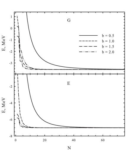
Fig. 1.: Convergence of the ground-state energy for the Gauss and exponential potentials

For all potentials, we take the radius of the potential $a=1$ fm, and the depth $V_{0}=-85$ MeV.  With such a choice of parameters, we obtain one bound state for all potentials, whose energies are listed in Table.  It was established by the numerical solution of the set of equations (20) with a maximal number of oscillator functions (see the text bellow).  One can see that we obtained a deeply bound state for the Yukawa potential, a weakly bound state for the Gaussian potential, and a moderately bound state for the exponential and square-well potentials.  The results demonstrated in Table are obtained with $N=300$ functions and the oscillator length $b=a=1.0$ fm.

Energy of the bound state

Potential	G	E	Y	SW
$E$, MeV	$-3.564$	$-7.006$	$-26.744$	$-9.388$

In what follows, we will use four values of the oscillator radius $b=0.5$, 1.0, 1.5, and 2.0 fm to study the dependence of the T-matrix expansion coefficients on the oscillator radius.  Calculations are organized in the following way.  First, we construct the $N\times N$ matrix of the Hamiltonian, where 1$\leq N\leq 500$.  (We do not dwell here on the calculations of matrix elements of the potential energy operator between oscillator functions.  We make use of the technique of generating functions, details of which can be found in Refs. [17,​ 18]).  Second, we calculate the eigenvalues (spectrum) and the eigenfunctions of the matrix by using the discrete form of the Schrödinger equation (20).  Then we obtain the T-matrix of bound and pseudobound states in the oscillator representation, by using Eq.  (34).  Third, we solve the system of linear equation (22), which determine the wave function and the phase shift of the scattering state with fixed energy $E,$ and then we construct the T-matrix by using Eq.  (34).  Finally, on the fourth step, we solve the set of linear equations (29) and obtain directly the T-matrix for a fixed energy $E$.  We make use of the third way to check the correctness of the calculations of the T-matrix in the fourth way.

In this section for the sake of convenience, we will denote the T-matrix as $t\left(p,E\right)$ explicitly indicating the energy of the discrete or continuous-spectrum state.

3.1 Convergence

First of all, we consider whether the oscillator basis is large enough to provide the convergent results for the bound state energy and the phase shift of continuous-spectrum states.  In Fig.  1, we show the dependence of the bound state energy $E$ on the number of oscillator functions $N$ involved in calculations.  These results are obtained for two potentials (Gaussian and exponential) and for four different values of oscillator length $b$.  One can see that one hundred functions give a very stable value of ground state energy for all oscillator lengths.  The dependence of the phase shift on the number of oscillator functions $N$ used in calculations is demonstrated in Fig.  2.  The phase shift is determined for the energy $E=5.0$ MeV.  The exact values of phase shift are calculated within the variable phase method [19,​ 20].  To obtain the stable phase shift independent of $N$, we need to use more oscillator functions than for bound state calculations.

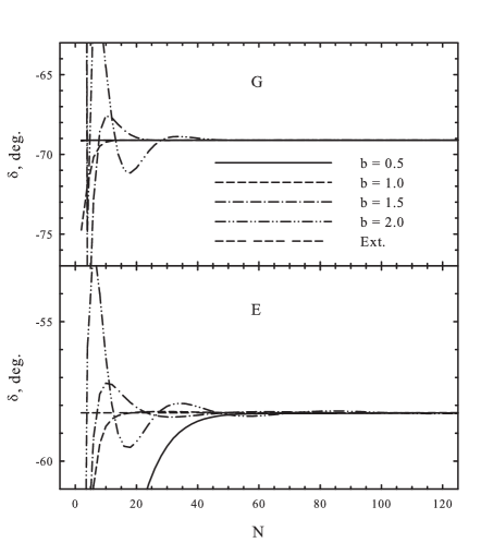
Fig. 2.: Phase shift as a function of the number of oscillator functions involved in calculations.  Results are obtained for the Gauss and exponential potentials with the energy $E=5.0$

3.2 Ground state

In this section, we consider the T-matrix of bound states.  In Fig.  3, we show the T-matrix for bound states with the Yukawa and exponential potentials. To demonstrate the rate of decreasing of the T-matrix expansion coefficients, we display the renormalized expansion coefficients $t_{n}/t_{0}=t_{n}\left(b,E\right)/t_{0}\left(b,E\right)$. For the Yukawa potential, the bound state is a deeply bound one with its energy to be $-26.74$ MeV.  This explains why the T-matrix for this potential decreases very rapidly, as $n$ increases.  The common feature of the T-matrix for the Yukawa and exponential potentials is that the larger the oscillator length $b$, the slower is the decreasing of the T-matrix expansion coefficients.  The same tendency is observed for the Gaussian and square-well potentials.

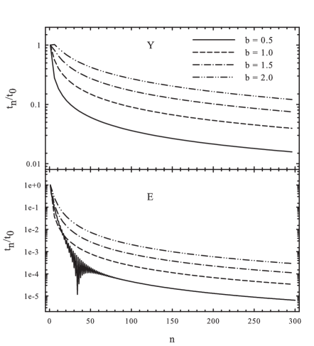
Fig. 3.: T-matrix for bound states calculated with the Yukawa and exponential potentials

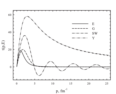
Fig. 4.: T-matrix of the bound state as a function of the momentum $p$ calculated with four potentials

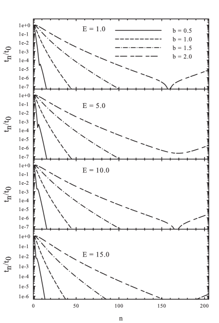
Fig. 5.: T-matrix expansion coefficients for continuous-spectrum states obtained with the Gaussian potential

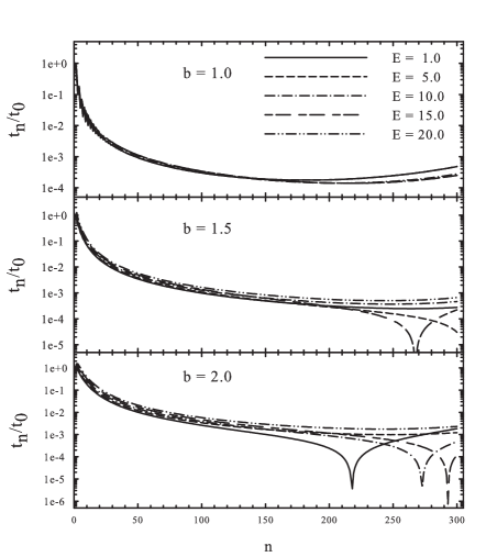
Fig. 6.: The T-matrix expansion coefficients as a function of $n$ calculated with the exponential potential

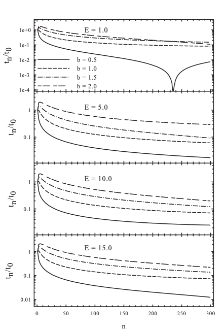
Fig. 7.: Expansion coeficients $t_{n}/t_{0}$, obtained with the Yukawa potential

With the help of relation (25), we can easily construct the T-matrix of a bound state in the momentum space.  In Fig. 4, we display the T-matrix $t\left(p,E\right)$ as a function of the momentum $p$ for the bound state for four potentials.  These results are obtained with the oscillator length $b=1$ fm and with $N=300$ oscillator functions.  However, by using other values of oscillator length, we obtain the same results.  It is worth to note that the T-matrix for a deeply bound state (Yukawa potential) is very dispersed in the momentum space.  This reflects the fact that the behavior of the T-matrix in the momentum space is determined by the wave function in the internal and asymptotic regions (see Eq.  (11)).  In some cases, the internal part of wave functions gives a larger contribution than the asymptotic part.  The same is true for the square-well potential, where the T-matrix is fully determined by the internal part of the wave function (as was pointed out above (see Eq.  (38))).  Contrary to the case of the Yukawa and square-well potentials, the T-matrix for the Gaussian and exponential potentials is represented by the small values of momentum $p$: $0\leq p\leq 7$ fm^-1.

3.3 Continuous-spectrum states

We selected five values of energy ($E=1$, 5, 10, 15, and 20 MeV) to study the dependence of the T-matrix expansion coefficients on the energy in the continuous spectrum.  The energy range $0<E\leq 20$ MeV selected in our calculations represents the region, where the effect of the potential energy is stronger than in the high-energy region.

As we are interested in the study of the rate of decreasing of $t_{n}$, we will display the renormalized expansion coefficients $\overline{t}_{n}=t_{n}/t_{0}$.  In Fig.  5, we show the T-matrix expansion coefficients for the Gauss potential for four values of energy $E=1$, 5, 10, and 15  MeV. One can see that $\overline{t}_{n}$ drops to zero very rapidly, as $n$ is increased.  The smaller the oscillator length, the faster is the decreasing of the T-matrix expansion coefficients for the Gauss potential.  Note that the rate of decreasing of $\overline{t}_{n}$ almost independent of the energy used in our calculations.

By comparing Fig.  5 with Figs. 6, 7, and 8, we can see that the fast decrease of expansion coefficients is observed only for the Gaussian potential, while the other potentials exhibit a much more slower decrease.

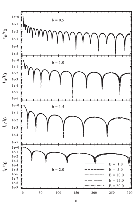
Fig. 8.: Square-well potential.  The renormalized T-matrix expansion coefficients as a function of $n$

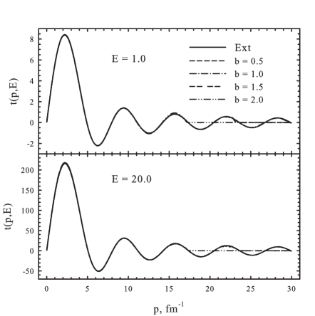
Fig. 9.: T-matrix convergence for the square-well potential calculated for two values of energy $E=1$ and $E=10$ MeV

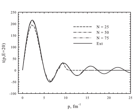
Fig. 10.: Convergence of the T-matrix for the square-well potential.  Results are obtained for $E=20.0$ MeV and with the oscillator length $b=1$ fm

Contrary to the Gaussian and square-well potentials, the T-matrix expansion coefficients for the exponential and Yukawa potentials are more strongly dependent on the energy.  This is explicitly demonstrated in Fig.  8, where the expansion coefficients for the T-matrix are displayed for a fixed oscillator length $b$ and for five different values of energy $E$.

The T-matrix as a function of the momentum $p$ for the square-well potential is shown in Fig.  9.  These results are obtained with $N=300$ oscillator functions.  In Fig. 9, we compare the calculated T-matrix with the exact one (marked as Ext) represented by Eq.  (39).  One can see that the calculated T-matrix coincides with the exact one in a wide range of momenta $p$.  The upper limit of the range depends on the number of functions $N$ and the oscillator length $b$ and, in view of the properties of oscillator functions, can be expressed as

$$p\leq\frac{\sqrt{4N+2L+3}}{b}.$$ (45)

Thus, the smaller the oscillator length, the larger is the range of momenta, which can be covered by $N$ oscillator functions.  Indeed, with $b=2.0$ fm, the nonzero values of the T-matrix are obtained for $p\leq$ $\leq 17$ fm^-1, which is in accordance with formula (45).

So far, to be on a safe side, we used the large basis of functions ($N=300$) to describe the bound and continuous-spectrum states.  Now, we are going to determine a minimal set of oscillator functions, which gives solutions with necessary precision.  We again turn our attention to the square-well potential, because the wave function and the T-matrix for this potential are obtained in a simple analytic form. This helps us to verify the precision of our calculations.  The exact (39) and calculated T-matrices determined with $N=25,$ 50, and 75 oscillator functions are shown in Fig.  10.  As is seen, 25 functions cannot provide with a good precision for the T-matrix.  The calculated T-matrix noticeably deviates from the exact one, whereas the T-matrix calculated with $N=50$ and $N=75$ is sufficiently close to the exact T-matrix.  We note that the larger the number of oscillator functions involved in calculations, the larger is the range of momenta $p$, where the T-matrix is described by these functions.  Note that this number of functions is consistent with the results presented in Figs.  1 and 2 as for the convergence of calculations of the bound state and the phase shift.

A similar picture is observed for the Gaussian and exponential potentials.  Unfortunately, we do not know the exact T-matrix for both of them.  For these potentials, the T-matrix calculated with $N=300$ oscillator functions can be considered as ‘‘exact’’, as this number of functions provides us with a stable solution and the exact phase shift.  With this definition, the calculations with $N=50$ and $N=75$ basis functions are almost indistinguishable for the ‘‘exact’’ T-matrix.  As for the Yukawa potential, one needs at least $N=125$ to be close to the ‘‘exact’’ T-matrix.

3.4 Asymptotics

In this section, we consider the asymptotic behavior of the T-matrix as a function of $n$ for large values of $n$.  In Refs. [1,​ 2], it was shown that the expansion coefficients for wave functions have the following asymptotic form:

$$C_{n}=\left\langle n|\Psi_{kL}\right\rangle\simeq\sqrt{2R_{n}}\Psi_{kL}\left(bR_{n}\right)\!.$$ (46)

Thus, the expansion coefficients $t_{n}=t_{nL}(b,k)$ for the T-matrix can be represented as

$$t_{n}=t_{nL}\left(b,k\right)=\left\langle\!n\left|\widehat{V}\right|\Psi_{kL}\!\right\rangle\simeq$$

$$\simeq\sqrt{2R_{n}}V\left(bR_{n}\right)\Psi_{kL}\left(bR_{n}\right)=V\left(bR_{n}\right)C_{n},$$ (47)

where

$$R_{n}=\sqrt{4n+2L+3}$$ (48)

is the turning point for a classical harmonic oscillator in the three-dimensional space.

In Ref.  [8] (see also [21]), it was discovered that there is another contribution (which was called as the short-range (SR) contribution, while the asymptotic term in Eqs.  (46) and (47) is called as the long-range (LR) contribution) to the asymptotic form, which relates the expansion coefficients $C_{n}$ and $t_{n}$ with the wave function and the T-matrix

$$\left\langle n|\Psi_{kL}\right\rangle\simeq\left(-1\right)^{n}\sqrt{2R_{n}}\Psi_{kL}\left(R_{n}/b\right)\!,$$ (49)

$$t_{nL}=\left\langle n\left|\widehat{V}\right|\Psi_{kL}\right\rangle\simeq\left(-1\right)^{n}\sqrt{2R_{n}}t_{L}\left(R_{n}/b,k\right)\!.$$ (50)

Equations (46) and (47) establish some relations between the expansion coefficients $C_{n}$ and $t_{n}$ and the wave function and the T-matrix for the large values of momentum $p=R_{n}/b$.

Let us consider the calculation of $t_{n}$ for the square-well potential in more details.  To determine $t_{n},$ one has to calculate the integral

$$t_{n}=t_{n}\left(b,k\right)=V_{0}\mathcal{A}_{kL}\sqrt{\frac{2}{\pi}}k\!\!\int\limits_{0}^{a}\!\!drr^{2}\Phi_{nL}\!\left(r,b\right)j_{L}\!\left(k_{0}r\right)=$$

$$=V_{0}\mathcal{A}_{kL}\sqrt{\frac{2}{\pi}}kb^{3}\!\!\int\limits_{0}^{a/b}\!\!d\rho\rho^{2}\Phi_{nL}\left(\rho,1\right)j_{L}\left(bk_{0}\rho\right)\!,$$

where $\rho=r/b$.  If $a/b\gg 1$ or $a/b>\sqrt{4n+2l+3}$, then the integral can be extended to infinity, and it gives the expansion coefficients for Bessel functions.  Thus, we obtain the long-range approximation.  For small values of the ratio $a/b\ll 1$ or $a/b\ll$ $\ll\sqrt{4n+2l+3}$, we can use the approximate formula for oscillator functions (Laguerre polynomials).

It was also demonstrated in [8] that, in some cases (which depend on the value of oscillator length $b$ and the shape of a potential), the SR contribution is much larger than the LR one.  In addition, one has to consider both of them in some cases. Unfortunately, we do not know the exact asymptotic form of the wave function $\Psi_{kL}(p)$ in the momentum space and the T-matrix for large values of $p$ as well.  It makes difficult to realize the short-range approximation.

Note that the knowledge of the asymptotics for the wave function and the T-matrix allowed us to formulate strategies (see Ref.  [7] and also Ref.  [10]) to obtain convergent results for the phase shift with a minimal set of oscillator functions.

We have explicit forms of the wave function and the T-matrix only for the square-well potential.  We will use it to check the asymptotic behavior of the T-matrix.

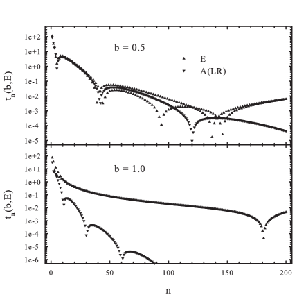
Fig. 11.: Exact (E) and asymptotic (A(LR)) forms of expansion coefficients $t_{n}$ calculated with the exponential potential for the energy $E=10.0$

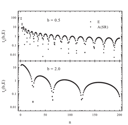
Fig. 12.: Expansion coefficient for the exact T-matrix (E) compared with the asymptotic short-range form (A(SR)). Calculations are made for $E=10.0$ with the square-well potential

In Fig.  11, we compare the calculated (E) and asymptotic long-range (A(LR)) forms of the T-matrix with the exponential potential.  As is seen, the asymptotic long-range form is valid for small values of $b$.  Starting from $b=1.0$, the asymptotic form is much smaller than the exact form.  A similar picture is observed for the Gaussian potential.  However, for the Yukawa and square-well potentials, the long-range form gives a very small contribution comparing with the exact form.

In Fig.  12, we demonstrate how the asymptotic short-range approximation works for the square-well potential.  We show results for two values of oscillator length $b$: the smallest ($b=0.5$) and largest ($b=2.0$) ones.  As is seen, the asymptotic short-range form is valid for small values of $b$.  For large values of $b,$ the asymptotic form coincides with the exact one for the whole range of the quantum number $n$.

It should be stressed that the long-range asymptotic form gives zero contribution to the presented results due to a specific shape of the square-well potential.

4 Conclusion

We have studied the properties of the T-matrix in the discrete oscillator representation.  It is demonstrated that the T-matrix in the oscillator representation can be presented in the vector and matrix forms.  The vector form is suitable for investigating the T-matrix on the half-on-shell space, while the matrix form is more appropriate for the full off-shell space.  The set of linear equations for the T-matrix expansion coefficients is deduced for both vector and matrix forms.

We calculated the T-matrix expansion coefficients for four different potentials.  It is shown that the rate of decreasing of the T-matrix expansion coefficients depends on the shape of a potential and on the oscillator length.  It is also shown that the T-matrix expansion coefficients slightly depend on the continuous-spectrum state energy.  We recall that the energy of scattering states is considered in the range $0\leq E\leq 20$, which is typical of the low-energy nuclear processes.

It is shown that the calculations of the T-matrix in the discrete representation is a reliable way for obtaining the information on the behavior of a quantum mechanical system.

We have investigated thoroughly the asymptotic properties of the T-matrix in the discrete space and established a relation with its asymptotic form in the continuous coordinate and momentum spaces.

The present discretization method can be easily extended for the T-matrix of real physical systems such as many-channel and many-cluster systems.

В.С. Василевський, М.Д. Солоха-Климчак
Т-МАТРИЦЯ В ДИСКРЕТНОМУ,
ОСЦИЛЯТОРНОМУ ПРЕДСТАВЛЕННI
Р е з ю м е
Дослiджено властивостi Т-матрицi для зв’язаних станiв та станiв неперервного спектра у дискретному, осциляторному представленнi. Дослiдження проводяться для модельної проблеми – частинка в полi центрального потенцiалу. Виведено систему лiнiйних рiвнянь, розв’язок яких визначає коефiцiєнти розкладу Т-матрицi по осциляторних функцiях. Ми вибрали чотири потенцiали (гаусiвський, юкавiвський, експоненцiальний та потенцiал прямокутної ями) для демонстрацiї особливостей Т-матрицi та її залежностi вiд форми потенцiалу. Ми також вивчаємо як коефiцiєнти розкладу Т-матрицi залежать вiд параметрiв осциляторного базису – осциляторної довжини та числа базисних функцiй, залучених у розрахунках.

References

- [1] G.F. Filippov and I.P. Okhrimenko, Sov. J. Nucl. Phys. 32, 480 (1981).
- [2] G.F. Filippov, Sov. J. Nucl. Phys. 33, 488 (1981).
- [3] E.J. Heller and H.A. Yamani, Phys. Rev. A 9, 1201 (1974).
- [4] H.A. Yamani and L. Fishman, J. Math. Phys. 16, 410 (1975).
- [5] The J-Matrix Method. Developments and Applications, edited by A.D. Alhaidari, H.A. Yamani, E.J. Heller, and M.S. Abdelmonem (Springer, Berlin, 2008).
- [6] O.A. Rubtsova and V.I. Kukulin, Phys. At. Nucl. 64, 1799 (2001).
- [7] F. Arickx, J. Broeckhove, P.V. Leuven, V. Vasilevsky, and G. Filippov, Amer. J. Phys. 62, 362 (1994).
- [8] V.S. Vasilevsky and F. Arickx, Phys. Rev. A 55, 265 (1997).
- [9] J. Broeckhove, V. Vasilevsky, F. Arickx, and A. Sytcheva, ArXiv Nuclear Theory e-prints, nucl-th/0412085 (2004).
- [10] J. Broeckhove, V.S. Vasilevsky, F. Arickx, and A.M. Sytcheva, in The J-Matrix Method. Developments and Applications, edited by A.D. Alhaidari, H.A. Yamani, E.J. Heller, and M.S. Abdelmonem (Springer, Berlin, 2008), p. 117.
- [11] R.G. Newton, Scattering Theory of Waves and Particles (McGraw-Hill, New York, 1966).
- [12] H. Friedrich, Scattering theory (Springer, Berlin, 2013).
- [13] Y.I. Nechaev and Y.F. Smirnov, Sov. J. Nucl. Phys. 35, 808 (1982).
- [14] E.J. Heller, Phys. Rev. A 12, 1222 (1975).
- [15] L.P. Kok, J.W. de Maag, H.H. Brouwer, and H. van Haeringen, Phys. Rev. C 26, 2381 (1982).
- [16] T. Dolinszky, J. Phys. G. Nucl. Phys. 10, 1639 (1984).
- [17] G.F. Filippov, V.S. Vasilevsky, and L.L. Chopovsky, Sov. J. Part. Nucl. 15, 600 (1984).
- [18] G.F. Filippov, V.S. Vasilevsky, and L.L. Chopovsky, Sov. J. Part. and Nucl. 16, 153 (1985).
- [19] F. Calogero, Variable Phase Approach to Potential Scattering (Academic Press, New York, 1967).
- [20] V.V. Babikov, Phase Function Method in Quantum Mechanics (Nauka, Moscow, 1976) (in Russian).
-
[21]
J. Broeckhove, F. Arickx, W. Vanroose, and
V.S. Vasilevsky, J. Phys. A Math. Gen. 37, 7769
(2004).
Received 18.07.14