Study of extremely reddened AGB stars in the Galactic bulge

Abstract

Context. Extremely reddened asymptotic giant branch stars (AGB) lose mass at high rates of $>$ 10^-5 M_⊙ yr^-1. This is the very last stage of AGB evolution, in which stars in the mass range $\sim$2.0 – 4.0 M_⊙ (for solar metallicity) should have been converted to C stars already. The extremely reddened AGB stars in the Galactic bulge are however predominantly O-rich, implying that they might be either low-mass stars or stars at the upper end of the AGB mass range.

Aims. Our goal is to determine the mass range of the most reddened AGB stars in the Galactic bulge.

Methods. Using Virtual Observatory tools, we constructed spectral energy distributions of a sample of 37 evolved stars in the Galactic bulge with extremely red IRAS colours. We fitted DUSTY models to the observational data to infer the bolometric fluxes. Applying individual corrections for interstellar extinction and adopting a common distance, we determined luminosities and mass-loss rates, and inferred the progenitor mass range from comparisons with AGB evolutionary models.

Results. The observed spectral energy distributions are consistent with a classification as reddened AGB stars, except for two stars, which are proto-planetary nebula candidates. For the AGB stars, we found luminosities in the range $\sim$ 3000 – 30,000 L_⊙ and mass-loss rates $\sim$ 10^-5 – $3\times 10^{-4}$ M_⊙ yr^-1. The corresponding mass range is $\sim$ 1.1 – 6.0 M_⊙ assuming solar metallicity.

Conclusions. Contrary to the predictions of the evolutionary models, the luminosity distribution is continuous, with many O-rich AGB stars in the mass range in which they should have been converted into C stars already. We suspect that bulge AGB stars have higher than solar metallicity and therefore may avoid the conversion to C-rich. The presence of low-mass stars in the sample shows that their termination of the AGB evolution also occurs during a final phase of very high mass-loss rate, leading to optically thick circumstellar shells.

1 Introduction

Low- and intermediate-mass stars pass along the asymptotic giant branch (AGB) towards the end of their evolution. Stellar evolution models predict that stars approaching the tip of the AGB experience thermal pulses. In this so-called ‘thermal pulses AGB’ (TP-AGB) phase, stars steadily increase in luminosities and mass-loss rates. This increase is interrupted on timescales of several ten thousand years by short-term variations due to the pulses. The heavy mass loss leads to the formation of circumstellar envelopes (CSE) of gas and dust. If the mass-loss rate surpasses $\dot{\rm{M}}$ $\geq$ 10^-6 M_⊙ yr^-1, the dust shell eventually becomes opaque to visible light (Habing, 1996). In addition, the stars may change their photospheric chemistry from O- to C-rich as a consequence of the so-called third dredge-up following a thermal pulse. The range of initial masses, in which the star will end as C-rich, depends on the metallicity. This range, defined on the main sequence, is 2 $\la$ M_MS $\la$ 4 M_⊙ for solar metallicities (Marigo & Girardi, 2007). At lower metallicities, as for example in the Magellanic Clouds, this mass range is extended to lower masses, significant increasing the fraction of C stars in the AGB population at the end of the TP-AGB phase (Blum et al., 2006). The stars ending the TP-AGB O-rich must have developed either from low-mass stars with main-sequence masses M_MS $\la$ 2 M_⊙ (Bertelli et al., 2008), for which the TP-AGB phase is terminated before the conversion is completed, or from intermediate-mass stars with M_MS $\ga$ 4 M_⊙, in which hot bottom burning (HBB) is active at the base of the convective envelope, preventing the formation of carbon.

Low-mass stars are expected to experience only moderate mass-loss rates during most of their AGB lifetime, leading to the formation of optically thin CSE. Low-mass AGB stars have been discovered predominantly in the optical and near-infrared wavelength range. Classical Mira variables belong to these kind of stars. AGB stars descending from progenitors with larger main-sequence masses are expected to be more luminous and to have higher mass-loss rates. They probably spend a larger fraction of their TP-AGB life in an optically obscured state (Mouhcine, 2002), which constrains their detection to the infrared or radio wavelength range. OH/IR stars, originally discovered by their radio OH maser emission and later identified in the infrared are an example of these kind of stars. OH maser emission is however also widespread among Mira variables, so that the term ‘OH/IR star’ encompasses low- and intermediate-mass stars.

If low-mass stars develop high mass-loss rates at the end of their evolution on the TP-AGB, they will form optically thick CSEs at lower mass-loss rates than intermediate-mass stars because they have more compact shells with smaller outflow velocities. Also, because of their frequency they should outnumber the intermediate-mass stars even among the obscured stars. However, in the Galactic disk, Chen et al. (2001) and Likkel (1989) found that the reddest (e.g. with highest mass-loss rates) OH/IR stars are dominated by progenies of main-sequence intermediate-mass stars. A dearth of low-mass stars among infrared bright sources in clusters of the Magellanic Clouds was also noted by van Loon et al. (2005). Therefore, low-mass stars may never evolve into the high mass-loss regime observed for the very red OH/IR stars, or it might be a very brief phase because the envelope mass above the core is rapidly depleted.

These stars should have relatively low luminosities, L $<$ 8000 L_⊙ for M_MS $\la$ 2 M_⊙ (Bertelli et al., 2008). Because of the uncertain distances in the Galactic disk and the strong variability, mean luminosities for AGB stars are difficult to determine and objects with relatively low luminosities are difficult to single out. A way to overcome this pitfall is to study AGB stars in the Galactic bulge, where a common distance can be used (van der Veen & Habing, 1990). AGB stars are luminous enough to be detectable there, especially in the mid-infrared. During their heavily obscured stage, they emit most of their radiation in the 10 – 30 $\mu$m range, which is less affected by the significant interstellar extinction towards many parts of the Galactic bulge.

The Galactic bulge is the central part of the Milky Way galaxy, consisting of a dominant old population of stars (t $>$ 8 Gyr; Zoccali et al. 2003; Vanhollebeke et al. 2009) and a smaller population of younger stars with no well constrained ages of $\sim$ 200 Myr – 7 Gyr (van Loon et al., 2003) or 1 – 3 Gyr (Groenewegen & Blommaert, 2005), to which the AGB stars in the Galactic bulge belong. In Baade’s window two metallicity populations have been found, of which the metal-poor population is associated with the old stellar population and the metal-rich population is consistent with a younger stellar population supporting a bar (Hill et al., 2011). A metallicity gradient was noted along the minor axis of the bulge (Zoccali et al., 2008) with the metallicity decreasing towards higher latitudes. No luminous C-rich AGB stars are known in the Galactic bulge (Blanco & Terndrup, 1989), suggesting that the younger stellar population in the Galactic bulge may be restricted to low-mass stars with AGB evolutionary timescales too short to experience enough dredge-ups to convert them into C stars (Buell, 2013). Then, the Galactic bulge OH/IR stars should also exclusively be descendants from low-mass stars, including the extremely red stars. This was implied by the findings of van der Veen & Habing (1990), who derived low progenitor masses of 1.0 – 1.4 M_⊙ for a sample of these red sources from the IRAS survey.

Although subsequent studies of AGB stars in the Galactic bulge also concluded that their samples originate from low-mass stars, luminosity distributions are not necessarily compatible with an exclusive origin from low-mass stars. For example, Glass et al. (2001) studied the variability properties of long-period, large-amplitude variable stars near the Galactic centre, and found a period-luminosity (P-L) relation that is compatible with the existence of a young population with initial masses in the range 2.5 – 3.0 M_⊙. In a later study on Mira variables in the optical gravitational lensing experiment (OGLE) bulge fields, Groenewegen & Blommaert (2005) found a different P-L relation, which they explained with a population with low initial masses (1.5 – 2.0 M_⊙). However, possibly more massive stars with P $>$ 700 days, such as obscured OH/IR stars, might have been missed in the I-band of the OGLE survey. Blommaert et al. (2006) studied a small sample of Galactic bulge AGB stars with near-infrared spectroscopy, and found a luminosity range from 1700 to 7700 L_⊙ with a mean of 4100 L_⊙, as expected for a population of AGB stars with low initial masses. Again, their study was restricted to objects with relatively low mass-loss rates, and may therefore have excluded more massive stars. This can be inferred from Ojha et al. (2007), who focussed their study on high mass-loss AGB stars, and found a wider luminosity distribution with a peak at 8000 L_⊙ and an appreciable number of sources with a luminosity exceeding 20,000 L_⊙.

A number of studies have been specifically focussed on OH/IR stars. Blommaert et al. (1998) and Wood et al. (1998) found that the OH/IR stars of the Galactic centre do not fit the classical Mira P-L relations (Feast et al., 1989; Whitelock et al., 1991). They systematically have lower luminosity and higher expansion velocity for a given period. OH/IR stars with periods as long as 1000 days, expected to have higher initial masses, were found to have low luminosities corresponding to Miras with masses below 1.5 M_⊙. These findings were explained by Wood et al. (1998) with a higher metallicity in the Galactic centre compared to the rest of the bulge. This fits into the general view that at low latitudes the metal-rich stellar population of the disk merges with the generally more metal-poor population of the bulge prevailing at larger latitudes. The origin from low-mass stars was confirmed by Ortiz et al. (2002) for other OH/IR stars observed by the ISOGAL survey. They concluded that the small number of objects more luminous than M_bol = –5.5 (L = 12,000 L_⊙) indicates that the initial masses of stars in the sample are rarely higher than $\sim$ 3 M_⊙, but instead the masses are about 1 – 2 M_⊙, on average.

All AGB star samples studied in the Galactic bulge were dominated by objects with blue or moderate reddened colours. This may have biased the studies towards low-mass objects, which would explain the scarcity of high-luminosity sources. In this paper, we study a sample of AGB stars of the Galactic bulge with extremely reddened colours. These stars are expected to be at the very end of the TP-AGB evolution. If low-mass stars evolve into the high mass-loss regime, the sample should include objects with rather low luminosities. If not, they must have originated from intermediate mass stars with correspondingly higher luminosities.

Currently, with new infrared surveys available, the spectral energy distributions (SED) of heavily obscured objects are covered with unprecedented coverage. Together with theoretical models of the CSEs of AGB stars, reliable bolometric fluxes can be derived without invoking uncertain bolometric corrections. Finally, it is also possible to obtain individual extinctions for each source leading to more reliable luminosities.

The sample of extremely reddened AGB stars is presented in Sect. 2. Section 3 describes the construction of the spectral energy distributions (SED), their fitting with DUSTY models, and the estimation of luminosities and mass-loss rates. The nature of the sources in the sample is discussed in Sect. 4, and the conclusions are presented in Sect. 5.

2 The sample

Our sample of AGB stars of the Galactic bulge (hereafter: GB sample) was selected from the sample of sources in Jiménez-Esteban et al. (2006). They studied around 100 IRAS sources distributed throughout the Milky Way with very red IRAS colours ($[12]-[25]$ $\geq$ 0.75 mag), located in a characteristic region of the IRAS two-colour diagram along the sequence of colours predicted for O-rich AGB stars with increasing mass loss (Bedijn, 1987), and having a high (VAR $>$ 50) IRAS variability index (Beichman et al., 1988). The high value of this index implies that all sources should be large-amplitude variables. By comparison with the colours of the ‘Arecibo sample’ of O-rich AGB stars (Jiménez-Esteban et al., 2005), they concluded that their sample of extremely reddened IRAS sources was also mainly made up of O-rich AGB stars highly obscured by their CSEs. To define the GB sample presented here, we selected the extremely reddened IRAS sources from Jiménez-Esteban et al. (2006) with angular distances $\leq$ 10^∘ from the Galactic centre.

Of the 39 sources selected in this region of the sky, two (IRAS 17317–3331 and IRAS 17411–3154) do not belong to the bulge. They are known to be foreground sources, located at a distance of 3.2 and 1.2 kpc, respectively (Cohen et al., 2005; Yuasa et al., 1999). The remaining 37 sources, presented in Table 1, define our sample of extremely reddened AGB stars in the Galactic bulge.

Although the sample is small, it is probably rather complete within its selection boundaries. Its flux density distribution at 25 $\mu$m peaks at $F_{25}$ $\sim$ 7 Jy, while the weakest source has $F_{25}$ $\sim$ 4 Jy (Table 2). AGB stars in the bulge matching the colour selection criterion $[12]-[25]$ $\geq$ 0.75 mag and $F_{25}$ $>$ 7 Jy are probably all contained in the sample, except those that are missing because of incompleteness of the IRAS catalogue. Surpassing the $F_{25}$ flux limit requires a minimum luminosity, which depends on the optical thickness of the CSE. This minimum luminosity is the lowest for sources in which the bulk of the emission is emitted in the 15–35 $\mu$m wavelength range. This minimum luminosity is also not biased by extinction, which is low at these wavelengths. As we show below, the minimum luminosity required to surpass the $F_{25}$ flux limit is low enough for high optical thickness, so that low-mass stars will also be present in the sample, if they develop the corresponding high mass-loss rates.

In accordance with the two foreground disk sources identified, we also expect contamination of the sample by background disk sources. The number of background disk sources can be roughly estimated as follows. Considering the foreground disk sources as “typical” for contaminating disk sources and using 4 Jy as the $F_{25}$ flux limit, all such disk sources within the solar orbit around the centre of the Milky Way should have been detected by IRAS. Assuming the same disk source density in front and behind the Galactic bulge, the number of foreground and background disk sources is coarsely proportional to the surface area of the Galactic disk segments in front and behind the bulge. Using a distance to the Galactic centre of 8.0 ($\pm$ 0.5) kpc (Reid, 1993), the adopted 10^∘ angular size of the Galactic bulge corresponds to a radius of $\sim$ 1.4 kpc. Based on this consideration, we expect $\sim$4 times more background sources than foreground sources. This yields about 8 sources out of 37, which could be background sources and whose luminosities would be underestimated in the following.

We searched in the literature for information on the predominant chemistry in the CSE of our objects. Six sources have IRAS Low Resolution Spectra (LRS) spectral classifications by Kwok et al. (1997). IRAS 17292–2727, IRAS 17316–3523, IRAS 17367–2722, IRAS 17418–2713, and IRAS 17495–2534 were classified as LRS class A, meaning that their spectra present the 9.7$\mu$m silicate dust feature in absorption. IRAS 18092–2347 was classified as LRS class I, meaning that the LRS was noisy or incomplete. For the rest of the sources, we searched for LRS spectra in the Calgary database. Only the LRS of IRAS 17367–3633 was found and visually classified. It shows a clear 9.7$\mu$m silicate dust feature in absorption. We also visually inspected the LRS of IRAS 18092–2347, which also showed the silicate dust feature in absorption. In addition, Golriz et al. (2014) have recently observed three of our sources that lack LRS classifications (IRAS  17251–2821, IRAS 17276–2846, and IRAS 17323–2424) with the Spitzer-Infrared Spectrograph. All three Spitzer spectra show the 9.7$\mu$m silicate in absorption. We classified these five sources as LRS class A.

Table 1: The GB sample. Observational parameters.

(1)	(2)	(3)	(4)	(5)	(6)	(7)	(8)	(9)	(10)	(11)	(12)	(13)	(14)	(15)
IRAS	WISE coordinates				IRAS				Radio datae			vexpf	AKs	Commentg
name	RA(J2000)	Dec(J2000)	Gal Long (∘)	Gal Lat (∘)	[12]-[25]a	[25]-[60]a	LRSb	Vard	OH	H2O	SiO	[km s-1]	mag
16582–3059	17:01:29.85	-31:04:19.1	352.843477	6.688608	0.89	–0.86		57	Y			13.4	0.15
17030–3053	17:06:14.06	-30:57:38.2	353.547542	5.945143	0.77	–0.73		99	Y			15.3	0.15
17107–3330	17:14:05.05	-33:33:57.9	352.421186	3.067547	0.86	–0.96		99	N				0.40
17128–3528	17:16:12.91	-35:32:12.8	351.072561	1.563949	1.52	0.12		98					0.82	NIR-Exc
17151–3642	17:18:29.53	-36:46:01.9	350.333858	0.477947	0.99	–0.30		99	N				1.63
17171–2955	17:20:20.35	-29:58:21.7	356.131283	4.050980	0.82	–1.30		99	N				0.30
17207–3632	17:24:07.27	-36:35:40.6	351.118359	–0.351526	0.95	0.46		99	Y	N		16.1	2.45
17251–2821	17:28:18.61	-28:24:00.5	358.413518	3.491327	0.94	–0.75	Ac	99	Y			16.0	0.35
17276–2846	17:30:48.32	-28:49:02.0	358.366433	2.804559	1.25	–0.12	Ac	79	Y			15.5	0.48	PPNc; DP
17292–2727	17:32:23.57	-27:30:01.2	359.662488	3.230668	0.81	–0.79	A	64	Y		Y	17.6	0.53	FIR-Exc
17316–3523	17:34:57.50	-35:25:52.5	353.298313	–1.536651	1.02	–0.72	A	99	Y			12.3	0.98
17323–2424	17:35:25.92	-24:26:30.5	2.611416	4.308932	0.99	–0.73	Ac	97	Y			13.8	0.60
17341–3529	17:37:30.29	-35:31:04.4	353.504370	–2.020286	0.88	–1.26		97	N		Y		0.50
17350–2413	17:38:08.86	-24:14:49.2	3.107790	3.890090	0.85	–1.50		99	Sp				0.32
17351–3429	17:38:26.28	-34:30:40.7	354.457640	–1.643595	0.95	–0.58		99	Y			20.0	0.56
17361–2358	17:39:14.82	-23:59:56.8	3.451800	3.809114	0.80	–0.88		99	N				0.31
17367–2722	17:39:52.43	-27:23:31.7	0.646949	1.889337	0.98	–0.47	A	97	Y			7.7	0.54	FIR-Exc
17367–3633	17:40:07.62	-36:34:41.4	352.888394	–3.033409	0.88	–0.75	Ac	92	Y			14.5	0.46	FIR-Exc
17368–3515	17:40:12.98	-35:16:40.8	354.002057	–2.360174	0.77	–0.71		99	Y			13.5	0.35
17392–3020	17:42:30.54	-30:22:07.4	358.425640	–0.174669	1.09	0.81		54	Y	Y,N		21.1	1.80
17418–2713	17:44:58.73	-27:14:42.7	1.369081	1.002630	1.34	–0.12	A	99	Y	N		15.2	0.76
17428–2438	17:45:56.94	-24:39:57.9	3.685349	2.159567	0.86	–1.04		73	Y			13.8	0.58
17495–2534	17:52:39.54	-25:34:39.1	3.684492	0.388289	0.80	–1.31	A	99	N			16.0f	1.28
17504–3312	17:53:50.25	-33:13:26.5	357.219129	–3.708828	1.17	0.21		84	Y			15.7	0.26	PPNc; DP
17521–2938	17:55:21.80	-29:39:13.0	0.471972	–2.191825	1.07	–0.17		98	Y			16.3	0.28
17545–3056	17:57:48.41	-30:56:25.8	359.621118	–3.292745	1.36	–0.04		89	Y			15.0	0.29
17545–3317	17:57:49.20	-33:17:47.6	357.573330	–4.466135	0.86	–0.91		99	Y			13.9	0.25
17583–3346	18:01:39.29	-33:46:00.5	357.556949	–5.393255	0.76	–0.99		99	Y			13.4	0.20	FIR-Exc
17584–3147	18:01:42.04	-31:47:54.7	359.284968	–4.439273	1.04	–0.53		99	Y			16.8	0.20
18019–3121	18:05:12.26	-31:21:43.2	0.032084	–4.878452	0.99	–1.00		99	Sp				0.21
18040–2726	18:07:08.92	-27:25:52.4	3.685892	–3.345684	1.05	–0.58		84	Y			16.3	0.19
18040–2953	18:07:18.44	-29:53:11.2	1.547809	–4.562185	0.82	–0.64		99	N				0.17
18091–2437	18:12:16.15	-24:36:42.9	6.715421	–2.997292	0.80	–0.60		99	Y			15.7	0.47
18092–2347	18:12:20.44	-23:46:55.9	7.452681	–2.614618	0.94	–0.15	I-Ac	92	Y	N		17.4	0.45
18092–2508	18:12:21.87	-25:07:20.6	6.276710	–3.260295	0.80	–0.80		91	Y			14.5	0.40	NIR-Exc
18195–2804	18:22:40.21	-28:03:08.8	4.760139	–6.667509	0.81	–0.70		99	Y			16.3	0.13
18201–2549	18:23:12.28	-25:47:58.7	6.828182	–5.738816	0.77	–1.50		98	N				0.16

• ^a IRAS colours as defined in Jiménez-Esteban et al. (2005); ^b IRAS Low Resolution Spectra; ^c Classification by this work (see Sections 2 and 3.1);^d IRAS variability index. ^e Radio data. Y: detection, N: no detection, Sp: single peak; ^f Expansion velocity from the OH maser velocity range, or from CO data for IRAS 17495–2534; ^g SED peculiarities (see Section 3.1). DP: double peaked, NIR-Exc: near-infrared excess, FIR-Exc: far-infrared excess, PPN: proto-planetary nebula candidate.

In addition, all sources of our sample except IRAS 17128–3528 were observed for OH maser emission (te Lintel Hekkert et al., 1991; David et al., 1993; Sevenster et al., 1997). Of these, eight were not detected, two (IRAS 17350–2413 and IRAS 18019–3121) presented single-peak OH emission, and the rest showed the typical double-peak spectrum commonly shown by OH/IR stars. Expansion velocities of the CSEs were derived for our objects from the velocity separations between the two OH peaks. For IRAS 17495–2534, with no OH maser emission detected, the expansion velocity was obtained from CO data (Loup et al., 1993). Four sources (IRAS 17207–3632, IRAS 17392–3020, IRAS 17418–2713, and IRAS 18092–2347) were observed for H₂O maser emission (Deacon et al., 2007; Suárez et al., 2007). Only IRAS 17392–3020 was detected by Deacon et al. (2007) in April 2003, although it was not detected two years later, in September 2005, by Suárez et al. (2007). Finally, two sources (IRAS 17292–2727 and IRAS 17341–3529) were detected as SiO masers (Nyman et al., 1998; Nakashima & Deguchi, 2003). Evidence for the O-rich nature of 30 sources is therefore provided by either detection of a maser and/or the presence of the silicate dust feature.

In Table 1 we present the observational parameters for the sources in our sample and summarise the above information. The IRAS object name is listed in the first column. Columns 2 to 5 give the equatorial and Galactic WISE coordinates (see Sect 3.1). Columns 6 and 7 give the IRAS colours. The IRAS LRS spectral classification and the IRAS variability index are given in the eight and ninth columns, respectively. In columns 10 to 12, we summarise the detection status for OH, H₂O, and SiO maser emission, respectively. The expansion velocity, if available, is listed in column 13, and the estimated individual extinction in the line of sight used to de-redden the observational photometry (see Sect. 3.2) is in column 14. Some comments on individual SEDs, discussed below, are given in the last column.

3 Analysis

3.1 Spectral energy distributions

To create the SEDs of the sources of our sample we collected, when available, photometric information from astronomical catalogues. To do that, we took advantage of the Virtual Observatory (VO). In particular, we made use of the Multiple Cone Search utility of Topcat, an interactive graphical viewer and editor for tabular data that allows the user to examine, analyse, combine, and edit astronomical tables. With Topcat, we cross-matched our sample with several available astronomical catalogues within the VO, using different search radii depending on the particular catalogue.

This way, we populated the SEDs from the near- to the far-infrared, wavelength range where these objects radiate the majority of their energy. We collected data from the following catalogues: Two Micron All Sky Survey (2MASS; Cutri et al. 2003) and VISTA variables in the Vía Láctea catalogue (VVV-DR1; Saito et al. 2012) at 1.25, 1.65, and 2.2 $\mu$m (filter J, H, and K_s, respectively); GLIMPSE (Churchwell et al., 2009) at 3.56, 4.51, 5.76, and 7.96 $\mu$m (filters I1, I2, I3, and I4, respectively); WISE catalogue (Wright et al., 2010) at 3.4, 4.6, 11.6, and 22.1 $\mu$m (filters W1, W2, W3, and W4, respectively); MSX6C Infrared Point Source Catalogue (Egan et al., 2003) at 8.28, 12.13, 14.65, and 21.3 $\mu$m (filters A, C, D, and E, respectively); AKARI Point Source Catalogue (Ishihara et al., 2010; Yamamura et al., 2010) at 9, 18, 65, 90, 140, and 160 $\mu$m (filters S09, S18, S65, S90, S140, and S160, respectively); and IRAS Point Sources Catalogue (Beichman et al., 1988) at 12, 25, 60 and 100 $\mu$m (filters 12, 25, 60, and 100, respectively). Since WISE data were not available through the VO, they were downloaded directly from the NASA/IPAC Infrared Science Archive.

We plotted the SED for each source and visually inspected them to check the consistency of the photometric data. When deviating photometric data were found, we used Aladin (Bonnarel et al., 2000), another VO tool, to visualise the astronomical images of the field and to check the reliability of the selected counterpart. Aladin allows users to visualise and analyse digitised astronomical images, and superimpose entries from astronomical catalogues or databases available from the VO services.

We found few inconsistencies, basically because of chance coincidences with field stars within our search radii. In all these cases the offending counterparts were removed. In the case of missing counterparts both in 2MASS and VISTA catalogues, we used a nearby ($<$30″) faint star to define an upper flux limit, preferably in the VISTA catalogue.

The photometric data are presented in Table 2, and the SEDs are plotted in Fig. 7. This figure shows the observational data after correcting for interstellar extinction and the DUSTY model that best fits the observations (see Sect. 3.2). Most of the sources present the typical SEDs of an AGB star heavily obscured by an optically thick CSE, with the maximum of their emission in the mid-IR. Note that most of the sources were not detected in the near-IR, or only barely in the K_s band.

Two sources (IRAS 17276–2846 and IRAS 17504–3312) show a peculiar double-peaked SED (Fig. 7). In the case of IRAS 17276–2846, the photospheric emission extends into the visual so that we added VVVDR1 data for filters Z (0.88 $\mu$m) and Y (1.02 $\mu$m) to the SED. These SEDs appear as soon as the mass-loss rates have greatly decreased and the obscuration has substantially diminished. The bluer peak at $\sim$ 2 $\mu$m is then attributed to the reddened stellar photosphere, and the redder peak corresponds to the emission at longer wavelengths by the cool circumstellar dust (e.g. see Fig. 9 in Sánchez Contreras et al., 2008). This kind of drop in mass-loss rate can be expected in the aftermath of a thermal pulse or when the stellar envelope has nearly been lost at the end of AGB evolution. Stars with this characteristic SED are generally considered to be proto-planetary nebula (PPN) (Oudmaijer, 1996), and therefore we assume that these stars have left the AGB. Since post-AGB evolution is outside the scope of the present paper, the two PPN candidates are not included in the following analyses.

Table 2: Photometric data collected.

Filter	J	H	$K_{\rm s}$	W1	I1	I2	W2	I3	I4	A	S09	W3	12	C
$\lambda$ ($\mu$m)	1.25	1.65	2.20	3.4	3.56	4.51	4.6	5.76	7.96	8.28	8.61	11.6	11.60	12.13
Flux in Jy $\times$	$10^{-4}$	$10^{-4}$	$10^{-4}$	$10^{-3}$	$10^{-3}$	$10^{-3}$	$10^{-2}$	$10^{-2}$	$10^{-2}$	$10^{-1}$	$10^{-1}$	$10^{-1}$	$10^{0}$	$10^{0}$
16582–3059	a2.6	a3.9	a25.1$\pm$1.3	138$\pm$3			77.3$\pm$1.6				20.5$\pm$0.2	23.1$\pm$0.4	2.5$\pm$0.2
17030–3053	a1.6	a1.8	a66.8$\pm$1.7	514$\pm$16			310$\pm$10			20.0$\pm$0.8	31.3$\pm$1.6	32.0$\pm$0.7	2.0$\pm$0.3	3.2
17107–3330	a4.0	a29.3$\pm$1.5	a609$\pm$16	680$\pm$20			270$\pm$9			20.3$\pm$0.8	47$\pm$3	34.2$\pm$0.7	2.60$\pm$0.16	2.87$\pm$0.16
17128–3528	a24	b1.52$\pm$0.14	b17.6$\pm$0.2	25.0$\pm$1.0			20.9$\pm$0.4			29.0$\pm$1.2	50$\pm$40	36.3$\pm$0.7	2.2$\pm$0.3	7.9$\pm$0.4
17151–3642	b0.2	b3.5	b0.7	132$\pm$4			69.0$\pm$1.6			47$\pm$2	20.3$\pm$0.2	30.4$\pm$0.6	5$\pm$2	7.1$\pm$0.4
17171–2955	b0.5	b20.2	b156.4$\pm$0.3	219$\pm$5			100$\pm$3			35.2$\pm$1.4	23.0$\pm$0.4	17.5$\pm$0.3	3.2$\pm$1.7	4.7$\pm$0.3
17207–3632	b0.2	b1.39	b38.9	43.7$\pm$1.6			163$\pm$5			56$\pm$2	54.7$\pm$0.7	104.7$\pm$1.2	6.2$\pm$1.2	8.8$\pm$0.4
17251–2821	a75	b12.1	b1.2	38.0$\pm$1.4	192$\pm$6	859$\pm$40	41.8$\pm$0.8	263$\pm$4	404$\pm$9	21.3$\pm$0.9		24.2$\pm$0.5	3.6$\pm$0.8	3.7$\pm$0.2
17276–2846d	a700$\pm$30	a1700	b1441.0$\pm$1.3	135$\pm$4	138$\pm$4	261$\pm$7	32.7$\pm$0.7	137$\pm$3	340$\pm$20	21.3$\pm$0.9		34.0$\pm$0.7	2.5$\pm$0.5	3.4$\pm$0.2
17292–2727	a70	a64	a63	870$\pm$30			780$\pm$30			80$\pm$3	88$\pm$12	145.1$\pm$0.8	11.6$\pm$0.6	11.4$\pm$0.6
17316–3523	b0.7	b1.1	a42$\pm$2	437$\pm$12			608$\pm$16			62$\pm$3	61$\pm$7	145.1$\pm$0.5	10$\pm$3	10.7$\pm$0.5
			b24.4$\pm$0.3
17323–2424	b0.4	b3.8	b0.6	24.2$\pm$0.9			44.1$\pm$0.9			23.4$\pm$1.0		30.6$\pm$0.6	3.4$\pm$0.5	2.9$\pm$0.2
17341–3529	a22.6$\pm$1.3	a316$\pm$8	a1590$\pm$30	1140$\pm$40			409$\pm$14			83$\pm$3	41$\pm$4	63.7$\pm$0.8	6.3$\pm$1.6	12.5$\pm$0.6
	b3.0$\pm$0.3	b67.0$\pm$0.4	b279.2$\pm$0.5
17350–2413	b0.7	b0.8	b175.7$\pm$0.3	178$\pm$4			63.8$\pm$1.3			14.8$\pm$0.6		12.9$\pm$0.2	3.6$\pm$1.3	1.99$\pm$0.13
17351–3429	b1.3	b1.8	a107$\pm$4	414$\pm$11			457$\pm$15			45$\pm$2		58.5$\pm$0.7	3.2$\pm$0.7	6.1$\pm$0.3
			b16.3$\pm$0.5
17361–2358	b0.5	b0.8	b19.2$\pm$0.3	253$\pm$7			253$\pm$7			19.6$\pm$0.8	63.5$\pm$0.8	49.2$\pm$0.4	3.6$\pm$0.8	2.70$\pm$0.15
17367–2722	b1.0	b1.1	b1.1	29$\pm$2			50$\pm$1			24.1$\pm$1.0		32.0$\pm$0.7	3.7$\pm$0.4	3.8$\pm$0.2
17367–3633	b0.3	b8.4$\pm$0.2	a66$\pm$2	690$\pm$20			710$\pm$20			62$\pm$3		147.2$\pm$1.0	8.8$\pm$1.1	8.2$\pm$0.4
			b43.9$\pm$0.4
17368–3515	b0.2	b1.2	b0.8	27.9$\pm$1.6			60.6$\pm$1.3			31.4$\pm$1.3		39.3$\pm$0.7	4.0$\pm$1.1	4.6$\pm$0.2
17392–3020	b0.2	b0.3	b1.0	74$\pm$5	37.7$\pm$1.5	350$\pm$20	80.7$\pm$1.8	179$\pm$3		40.1$\pm$1.6	20.30$\pm$0.03	33.9$\pm$0.7	6.3$\pm$0.5	5.2$\pm$0.3
17418–2713	b1.0	b1.3	b2.0	40$\pm$3	22.6$\pm$1.0	490$\pm$30	175$\pm$4	368$\pm$7		179$\pm$7	179.3$\pm$0.6	384.4$\pm$1.1	15$\pm$3	29.8$\pm$1.5
17428–2438	b0.9	b1.1	b20.6$\pm$0.4	292$\pm$8	246$\pm$8	630$\pm$40	308$\pm$9	240$\pm$5		36.6$\pm$1.5	45$\pm$15	57.0$\pm$0.6	6.6$\pm$0.4	4.73$\pm$0.13
17495–2534	b0.3	b0.3	b144.3$\pm$0.5	1108$\pm$49	370$\pm$20	8400$\pm$800	1140$\pm$30	436$\pm$11		85$\pm$4		314.5$\pm$1.2	29$\pm$5	13.7$\pm$0.7
17504–3312	b54.1$\pm$0.3	a70.3$\pm$1.4	a209$\pm$4	59$\pm$2			11.4$\pm$0.3			7.3$\pm$0.3	6.97$\pm$0.05	18.1$\pm$0.3	4.1$\pm$0.8	2.42$\pm$0.15
		b193.1$\pm$0.4	b425.8$\pm$0.4
17521–2938	a31	a44	b2.3	3.6$\pm$1.7	29.2$\pm$1.5	269$\pm$9	16.5$\pm$0.4	130$\pm$3		15.2$\pm$0.6	26$\pm$6	18.3$\pm$0.4	3.1$\pm$0.6	2.36$\pm$0.12
17545–3056	b1.3	b1.4	b1.6	2.2	1.52$\pm$0.08	31.6$\pm$1.2	5.72$\pm$0.16	33.4$\pm$0.7	119$\pm$3	11.1$\pm$0.5		22.4$\pm$0.4	2.9$\pm$0.4	2.53$\pm$0.13
17545–3317	b0.8	b1.3	a45$\pm$3	204$\pm$5			140$\pm$4			46$\pm$2		32.7$\pm$0.6	3.6$\pm$0.3	6.2$\pm$0.3
			b11.4$\pm$0.3
17583–3346	b25.8$\pm$0.2	a39$\pm$2	a522$\pm$9	631$\pm$19			210$\pm$6					36.2$\pm$0.7	2.00$\pm$0.14
		b265.1$\pm$0.2	b1082.0$\pm$1.0
17584–3147	b0.7	b0.7	b1.0	46.9$\pm$1.6			95$\pm$2			22.6$\pm$0.9		67.7$\pm$0.8	6.9$\pm$1.0	3.4$\pm$0.2
18019–3121	b0.5	b0.7	b0.8	25.2$\pm$0.9			50.0$\pm$1.0			24.5$\pm$1.0	28$\pm$4	29.3$\pm$0.6	3.5$\pm$1.1	3.0$\pm$0.2
18040–2726	b1.1	b1.1	b0.8	39.1$\pm$1.3			97$\pm$2			24.2$\pm$1.0	51$\pm$15	59.4$\pm$0.9	6.5$\pm$0.5	3.5$\pm$0.2
18040–2953	b0.9	b1.0	b8.6$\pm$0.3	345$\pm$9			492$\pm$17			28.3$\pm$1.2	30$\pm$4	84.4$\pm$0.6	5.0$\pm$0.8	3.7$\pm$0.2
18091–2437	b0.8	b0.7	b10.6$\pm$0.3	177$\pm$4	236$\pm$8		150$\pm$4	212$\pm$5		16.3$\pm$0.7	20.2$\pm$0.9	32.8$\pm$0.7	4.6$\pm$0.7	2.30$\pm$0.14
18092–2347	b0.5	b1.0	b1.0	4.3$\pm$1.1	13.9$\pm$0.6	279$\pm$13	36.5$\pm$0.7	230$\pm$5		50$\pm$2	55$\pm$3	121.2$\pm$0.9	10.9$\pm$0.8	9.8$\pm$0.5
18092–2508	b1.5$\pm$0.2	b2.4$\pm$0.3	b20.2$\pm$0.3	311$\pm$9			352$\pm$13			49$\pm$2	51.8$\pm$7	58.4$\pm$0.5	5.6$\pm$0.7	6.6$\pm$0.3
18195–2804	a0.4	b0.5	b21.76$\pm$0.16	362$\pm$8			341$\pm$10				20.6$\pm$6	49.2$\pm$0.5	3.6$\pm$0.8
18201–2549	a11.1$\pm$0.7	a323$\pm$7	a3260$\pm$60	2340$\pm$140			678$\pm$16				93.627$\pm$0.003	95.0$\pm$0.5	5.0$\pm$0.7
	b14.22$\pm$0.18	b366.9$\pm$0.3	b2759$\pm$3

• Data without errors are upper limits; ^a 2MASS data; ^b VVV-DR1 data; ^c No confirmed detection; ^d VVV-DR1 fluxes in Jy $\times$ 10^-5: F_z=761$\pm$2 and F_Y=3017$\pm$4.

Table 2: Photometric data collected. Continued

Filter ($\lambda$ ($\mu$m))	D	S18	E	W4	25	60	S65	S90	100	S140	S160
$\lambda$ ($\mu$m)	14.65	18.39	21.3	22.1	23.88	60	65	90	100	140	160
Flux in Jy $\times$	$10^{0}$	$10^{-1}$	$10^{0}$	$10^{-1}$	$10^{0}$	$10^{0}$	$10^{0}$	$10^{-1}$	$10^{0}$	$10^{0}$	$10^{0}$
16582–3059				51.7$\pm$0.9	5.8$\pm$0.6	2.6$\pm$0.3	c1.6	13$\pm$2	20		c1.3
17030–3053	3.5$\pm$0.2		5.5	58.0$\pm$0.8	4.1$\pm$0.7	2.1$\pm$0.2			26
17107–3330	3.4$\pm$0.2		3.8$\pm$0.2	64.9$\pm$0.8	5.7$\pm$1.0	2.4$\pm$0.5			20
17128–3528	13.0$\pm$0.8	93.0$\pm$0.3	13.8$\pm$0.8	114.9$\pm$1.5	9.1$\pm$1.4	10.1$\pm$0.8	17$\pm$5	86$\pm$8	55	c9.9	c7.3
17151–3642	11.2$\pm$0.7		11.3$\pm$0.7	73.2$\pm$1.6	13$\pm$4	10.1$\pm$1.6	c6.8	71$\pm$5	320	c30$\pm$4	c82$\pm$7
17171–2955	5.8$\pm$0.4		6.1$\pm$0.4	33.6$\pm$0.3	7$\pm$4	2.1$\pm$0.6	c1.1	16.5$\pm$0.2	18
17207–3632	15.4$\pm$0.9		12.6$\pm$0.8	194$\pm$3	15$\pm$3	23$\pm$3	16$\pm$4	113$\pm$6	1500		c45$\pm$9
17251–2821	4.9$\pm$0.3	47$\pm$8	5.8$\pm$0.4	58.8$\pm$0.7	8.5$\pm$1.6	4.2$\pm$0.4	c1.7$\pm$0.6	22$\pm$2	20	c1.8
17276–2846d	5.7$\pm$0.4	59.20$\pm$4	5.4$\pm$0.3	75.7$\pm$0.9	7.9$\pm$0.9	7.2$\pm$0.8	c6.2	37$\pm$3	30	c1.4
17292–2727	16.1$\pm$1.0	153.3$\pm$0.7	19.5$\pm$1.2	213$\pm$6	24$\pm$2	11.8$\pm$1.1	8.9$\pm$0.4	71$\pm$9	12	4.6$\pm$1.2	c4.4
17316–3523	16.4$\pm$1.0		19.6$\pm$1.2	246$\pm$4	25$\pm$4	13$\pm$2			170
17323–2424	5.5$\pm$0.3	43.0$\pm$1.6	7.1$\pm$0.5	67.9$\pm$0.9	8.5$\pm$1.7	4.3$\pm$0.5	c3.8	19$\pm$4	13		c0.66
17341–3529	13.3$\pm$0.8	87$\pm$10	16.4$\pm$1.0	116.9$\pm$1.3	14$\pm$2	4.5$\pm$0.9			100
17350–2413	2.76$\pm$0.18		3.1	27.6$\pm$0.3	7.8$\pm$0.6	2.0$\pm$0.2	c1.4	13.1$\pm$0.6	13	c0.61
17351–3429	8.6$\pm$0.5	106.9$\pm$1.6	10.2$\pm$0.6	117.1$\pm$1.1	7.8$\pm$1.4	4.6$\pm$0.7	6.0$\pm$0.8	29$\pm$6	160	c2.0	c0.13
17361–2358	3.7$\pm$0.2		4.1$\pm$0.3	85.9$\pm$1.7	7.5$\pm$1.4	3.3$\pm$0.4			11
17367–2722	6.1$\pm$0.4	90$\pm$30	6.6$\pm$0.4	76.7$\pm$1.3	9.2$\pm$1.2	6.0$\pm$0.5	c4.0	44$\pm$7	36	c4.4$\pm$1.1	c4.7
17367–3633	11.6$\pm$0.7		13.3$\pm$0.8	204$\pm$4	20$\pm$2	9.9$\pm$1.0	11$\pm$5	69.6$\pm$0.4	10	c6$\pm$4	c0.92
17368–3515	7.3$\pm$0.5	74.3$\pm$1.3	7.5$\pm$0.5	85.0$\pm$1.0	8$\pm$2	4.2$\pm$1.0	c5.9$\pm$1.5	21$\pm$3	13
17392–3020	9.0$\pm$0.5	90$\pm$30	9.4$\pm$0.6	91.6$\pm$1.6	17.3$\pm$1.6	36$\pm$7			210
17418–2713	58$\pm$4		68$\pm$4	720$\pm$9	51$\pm$7	46$\pm$5			500
17428–2438	6.3$\pm$0.4	103.5$\pm$1.1	7.2$\pm$0.4	110.5$\pm$1.7	14.6$\pm$1.2	5.6$\pm$0.6			47
17495–2534	19.9$\pm$1.2	500$\pm$40	23.7$\pm$1.4	521$\pm$8	61$\pm$8	18$\pm$2	17$\pm$4	88.9$\pm$1.7	370
17504–3312	4.7$\pm$0.3	59.34$\pm$0.13	7.8$\pm$0.5	87.6$\pm$1.0	12.0$\pm$1.2	15$\pm$2			43
17521–2938	4.3$\pm$0.3	69$\pm$13	5.4$\pm$0.3	49.8$\pm$0.7	8.2$\pm$1.7	7.0$\pm$1.1			110
17545–3056	5.5$\pm$0.3	50$\pm$20	6.5$\pm$0.4	75.6$\pm$0.9	10.2$\pm$0.9	9.8$\pm$1.2	5.3$\pm$1.2	c45.56	57	c7.0	c0.25
17545–3317	7.9$\pm$0.5		9.1$\pm$0.6	50.1$\pm$0.5	8.0$\pm$1.1	3.5$\pm$0.4	c1.7	14$\pm$2	34		c0.42
17583–3346		35.0$\pm$0.8		59.0$\pm$0.6	4.0$\pm$0.3	1.6$\pm$0.4	c1.1	13.0$\pm$1.6	26	c1.0
17584–3147	5.1$\pm$0.3	99$\pm$17	6.6$\pm$0.4	167$\pm$4	18$\pm$3	11.0$\pm$1.3	6.82$\pm$0.13	c43.67	12
18019–3121	5.7$\pm$0.4	69.17$\pm$0.04	5.2$\pm$0.3	64.5$\pm$0.8	9$\pm$2	3.4$\pm$0.9			62
18040–2726	6.5$\pm$0.4	130$\pm$20	6.4$\pm$0.4	137$\pm$2	17.0$\pm$1.4	9.9$\pm$1.2	8.8$\pm$0.4	69$\pm$3	66	c1.7	c1.1
18040–2953	5.7$\pm$0.4	60$\pm$7	6.3$\pm$0.4	143$\pm$2	11$\pm$2	5.9$\pm$1.0	c2.9	25.01$\pm$0.02	42		c1.7
18091–2437	3.1$\pm$0.2		3.8$\pm$0.2	63.8$\pm$0.7	9.7$\pm$1.5	5.6$\pm$0.6			86
18092–2347	17.7$\pm$1.1		18.1$\pm$1.1	245$\pm$5	26$\pm$2	22.4$\pm$3	13.2$\pm$0.3	115$\pm$7	110		c4.7
18092–2508	9.5$\pm$0.6	121.0$\pm$0.9	10.6$\pm$0.7	115$\pm$2	11.8$\pm$1.1	5.6$\pm$0.7	c4.7	26.9$\pm$0.9	90	c0.79	c2.0
18195–2804		30.4$\pm$0.5		95.1$\pm$1.7	7.7$\pm$1.5	4.0$\pm$0.5	1.7$\pm$0.3	16$\pm$2	17	c0.6$\pm$0.8	c1.4
18201–2549		64.9$\pm$0.4		133.7$\pm$1.1	10.2$\pm$1.4	2.6$\pm$0.2	c1.2	13$\pm$3	23		c1.3

• Data without errors are upper limits; ^a 2MASS data; ^b VVV-DR1 data; ^c No confirmed detection; ^d VVV-DR1 fluxes in Jy $\times$ 10^-5: F_z=761$\pm$2 and F_Y=3017$\pm$4.

3.2 Observed bolometric flux

The bulge sample of AGB stars is nowadays covered over a large part of their SED by a multitude of infrared surveys. This allows us to determine the bolometric flux with much higher accuracy compared to earlier times, when (uncertain) bolometric corrections or (unsuitable) black-body fitting had to be applied to cover the unobserved parts of the SED (e.g. van der Veen & Breukers, 1989; Ortiz et al., 2002). However, the photometric data available is not complete for all sources so that a determination of the bolometric flux by integration of an interpolated curve between the available data points will be unsatisfactory. Also bolometric corrections (although small ones) for the spectral ranges outside the infrared are still required. We therefore decided to fit the observed SEDs with models of stars obscured by a dusty radial symmetric CSE and to determine the bolometric fluxes from the models. Because of the large distance of the Galactic bulge, the stars may be observed through large columns of intervening dust, such that extinction may have a noticeable influence on the shape of the SEDs and on the observed bolometric flux.

To de-redden the photometric data, we corrected the flux at 2.2 $\mu$m ($K_{S}$ band) using the extinction maps towards the Galactic bulge given by Gonzalez et al. (2012). The absolute extinctions towards the sources of our sample are 0.13 $\leq$ A_Ks $\leq$ 2.45 mag (see Table 1). Two sources (IRAS 16582–3059 and IRAS 17030–3053) are not covered by the maps and we assigned $A_{Ks}$ = 0.15 mag to them. About half of the sources are also covered by the extinction maps of Nidever et al. (2012). Their absolute extinctions are 0.14 $\pm$ 0.04 mag higher for $A_{Ks}$ $<$ 1.0 mag than those of Gonzalez et al. (2012). Because the uncertainties given in both papers are 0.1 mag, we considered this difference as not significant. For higher extinctions, the scatter $\sigma$ between the maps is larger with $\sigma$ = 0.3 mag.

To correct the other photometric bands, we determined the extinction coefficients A_λ/A_Ks from the extinction curves given by Chen et al. (2013) up to $\lambda$ = 8 $\mu$m and from Gao et al. (2009) up to 24 $\mu$m. The extinction coefficients beyond $\lambda$ = 24 $\mu$m were determined by extrapolation using a power law with $\beta$ = –1.7.

The de-reddened SEDs were modelled using the radiation transport code DUSTY (Ivezić et al., 1999). Because the observed photometry taken at different epochs is likely affected by variability, the photometric data are expected to scatter around the mean SED. The relatively sparse coverage of the SEDs with photometry and the variability preclude the determination of accurate models. We therefore decided to use a standard model, in which most of the parameters are fixed, and only the optical depth of the shell was left as variable parameter.

Combining the information from the IRAS LRS classifications and the maser detections, O-rich chemistry can be inferred for 28 objects. Carbon stars are extremely rare in the Galactic bulge (Blanco & Terndrup, 1989). Hence, we decided to assume O-rich chemistry for the remaining seven objects, following Lewis (1992), who found that infrared sources without OH maser detection but with IRAS colours similar to those of OH/IR stars are most probably O-rich variable AGB stars. Consequently, we only used models with O-rich chemistry.

The standard model assumes a central star with an effective temperature T_eff = 2500 K, and a dust condensation temperature T_d = 1000 K. We used the optical constants for amorphous cold silicates from Ossenkopf et al. (1992) and took the standard MRN (Mathis et al., 1977) dust size distribution with $n(a)$ $\propto$ $a^{-3.5}$, where $n$ is the number density and $a$ is the size of the grains. The grain sizes were limited to 0.005 $\leq$ $a$ $\leq$ 0.25 $\mu$m. The inner radius $R_{min}$ of the CSE is determined by DUSTY from the dust condensation temperature assumed. The outer radius of the shell was set to $R_{max}$ = 100 $R_{min}$. Instead of describing the density distribution in the shell by an analytic profile, the option to calculate the wind structure from hydrodynamics was chosen, which allows us to determine mass-loss rates from the models (Ivezic & Elitzur, 1995). Models were calculated for optical depths 0.2 $<$ $\tau_{9.7\mu m}$ $<$ 50 and the best model was found by minimising the deviations from the de-reddened flux densities. In several cases two models were fitted representing the star at different variability states. Because of the requirement of a very red IRAS colour, most stars possess a CSE with a high optical depth $\tau_{9.7\mu m}$ $>$ 10, and only four have 5 $<$ $\tau_{9.7\mu m}$ $<$ 10. The bolometric fluxes determined vary by a factor 20 and are in the range $f_{bol}$ = $10^{-12}$ – $2\times 10^{-11}$ Watt m^-2.

The results are given in Table 3. It lists the object name in the first column. The best-fit optical depth $\tau_{9.7\mu m}$, and the bolometric flux $f_{bol}$ delivered by DUSTY are given in the two following columns. The last two columns give luminosities and mass-loss rates discussed in the next Section.

The uncertainties of $\log f_{bol}$ are approximately 0.2 dex, which we attribute mostly to variability. For the cases where models for different variability states are given, the difference is $\sim$ 0.3 dex. We conclude therefore that the peak-to-peak luminosity variation of the large-amplitude variable objects is $\geq$ 2. This number is probably a lower limit, as Suh (2004) determined for two extremely obscured OH/IR stars in the Galactic disk luminosity variations by a factor 3 – 3.6. The bolometric fluxes determined here cannot be individually corrected for variability, but in general we expect them to be close to the mean bolometric fluxes. The deviations of the observed bolometric fluxes from the mean fluxes is at most half of the peak-to-peak variations, and very likely even lower in those cases where average bolometric fluxes are available from fits at different variability states.

The de-reddened SEDs and the models are shown in Fig. 7. The observed SEDs are the result of the emission from the circumstellar dust with high optical depths, which in addition are reddened further by interstellar extinction. The removal of the interstellar extinction makes the SEDs bluer and brighter than the observed SEDs. As an example, the influence of extinction on photometry and model fit is shown in Fig. 1 for IRAS 17392$-$3020. We found that the increase in logarithmic bolometric flux surpasses 0.2 dex only if A_Ks $>$ 1.0 mag, which applies for four sources in the sample. Therefore, the largest contributions to the uncertainties of the $f_{bol}$ determination is in general from the variability and not from interstellar extinction.

For several sources the DUSTY models predict less flux than observed in the near infrared at $\lambda$ $<$ 3 $\mu$m and in the far infrared at wavelengths 60 $<$ $\lambda$ $<$ 160 $\mu$m. These sources are marked in Table 1 as ‘NIR-Exc’ and ‘FIR-Exc’. The observed excess emission makes only a minor contribution to the overall luminosity and has been neglected for the luminosity determination.

The near-infrared excess presented by IRAS 17128–3528 and IRAS 18092–2508 (see Fig. 7) is evident from the unexpectedly high brightness in the J, H, and K filters measured by the VVV-DR1 survey. We verified that this is not due to missidentification or contamination of neighbouring objects. These stars may have developed deviations of their dust distribution from spherical symmetry or their circumstellar shell may have been diluted after the end of the strong AGB mass loss, so that the light of the central star could escape to form the excess. They might currently be starting the post-AGB evolution and may later develop double-peaked SEDs as seen in the PPN candidates IRAS 17276–2846 and IRAS 17504–3312 (cf. Sect. 3.1). Alternatively, they might belong to binary systems, where the excess emission comes from the companion. In any case, additional photometry is required to verify the near-IR excesses for these sources.

The SEDs of IRAS 17292–2727, IRAS 17367–2722, IRAS 17367–3633, and IRAS 17583–3346 (Fig. 7) present a far-infrared excess. This far-infrared excess emission can not be attributed to photometric errors or variability since consistent flux densities have been measured at different times by more than one survey. Such excess emission has been seen before in a number of objects, in which the excess can be followed over a large wavelength interval extending up to the submillimeter and millimeter ranges. To account for the excess flux an additional dust component of larger cool grains is required to model the SEDs of these stars (Sánchez Contreras et al., 2007).

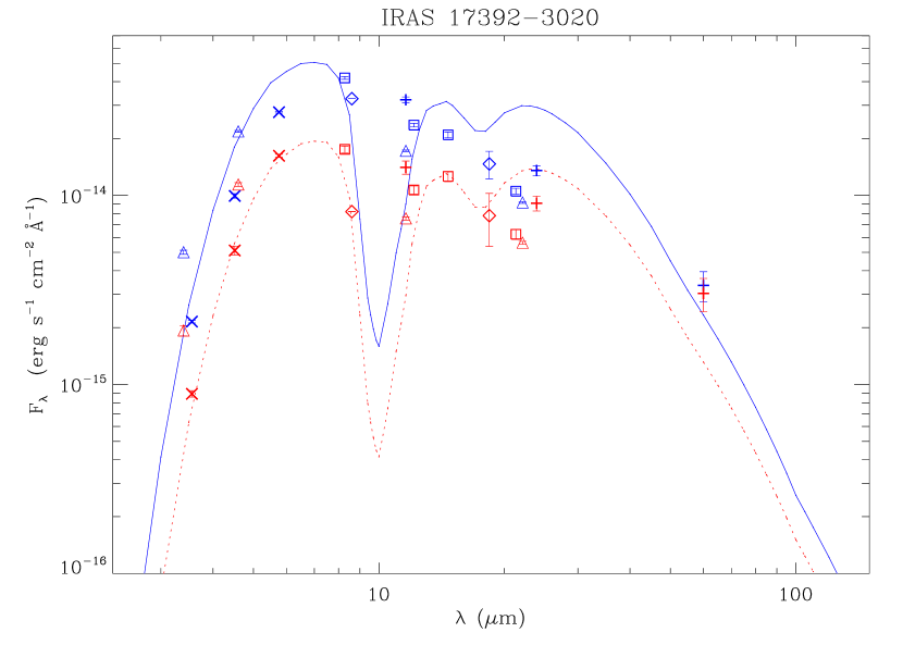
Figure 1: Observational photometry and model fits of IRAS 17392$-$3020. For each photometric observation, the uncorrected flux density (lower red symbols) and the de-reddened flux density for A_Ks = 1.8 mag (upper blue symbols) are given. The best-fitting models are given as dotted (red) curve for the observed photometry and as solid (blue) curve for the de-reddened photometry. The de-reddened bolometric flux is a factor 2.2 enhanced. Symbols are as in Fig. 7.

Table 3: Result of the DUSTY model fit.

(1)	(2)	(3)	(4)	(5)
IRAS	$\tau_{9.7\mu m}$	$-$log($f_{bol}$)a	Lb	$\dot{\rm{M}}$
name			$\times$$10^{3}$ L⊙	$\times$$10^{-5}$ M⊙ yr-1
16582–3059	15.9	11.70	4.0	1.7
17030–3053	10.9	11.75	3.5	1.0
17107–3330c	6.2	11.64	4.5	1.0
17128–3528c	41.3	11.30	9.9	8.7
17151–3642c	23.4	11.25	11.1	6.0
17171–2955c	10.9	11.63	4.7	1.4
17207–3632	34.2	11.00	19.8	12.8
17251–2821	23.3 – 28.2	11.44 – 11.80	7.2 – 3.1	1.7 – 3.4
17292–2727	15.9	11.05	17.7	5.7
17316–3523	15.9	11.08	16.5	7.6
17323–2424	28.2	11.67	4.2	2.7
17341–3529c	5.1 – 6.2	11.05 – 11.30	17.7 – 9.9	2.1 – 3.4
17350–2413c	9.0 – 10.9	11.50 – 11.95	6.3 – 2.2	0.7 – 1.7
17351–3429	13.2	11.30	9.9	2.4
17361–2358c	15.9	11.57	5.3	2.1
17367–2722	34.2	11.60	5.0	6.8
17367–3633	10.9 – 13.2	10.80 – 11.15	31.4 – 14.0	4.7 – 9.3
17368–3515	28.2	11.56	5.5	3.6
17392–3020	41.3	11.01	19.4	11.3
17418–2713	50.0 – 50.0	10.67 – 11.02	42.4 – 18.9	18.0 – 40.4
17428–2438	15.9	11.40	7.9	3.2
17495–2534	15.9 – 28.2	10.70 – 11.00	39.6 – 19.8	11.1 – 14.0
17521–2938	41.3 – 50.0	11.60 – 11.88	4.9 – 2.6	2.3 – 3.7
17545–3056	50.0	11.77	3.4	3.3
17545–3317	15.9	11.50	6.3	2.6
17583–3346	5.1	11.40	7.9	1.6
17584–3147	34.2	11.45	7.0	4.3
18019–3121c	28.2	11.71	3.9	2.5
18040–2726	34.2 – 34.2	11.35 – 11.65	8.9 – 4.4	2.8 – 5.7
18040–2953c	19.3 – 23.3	11.30 – 11.65	9.9 – 4.4	2.4 – 4.6
18091–2437	15.9 – 19.3	11.50 – 11.85	6.3 – 2.8	1.2 – 2.3
18092–2347	50.0	11.19	12.8	10.6
18092–2508	19.3	11.35	8.9	4.0
18195–2804	15.9	11.55	5.6	1.9
18201–2549c	5.1	11.25	11.2	2.2

• ^a $f_{bol}$ in Watt m^-2; ^b Luminosity estimated using the distance of 8.0 kpc to the Galactic centre. ^c v_exp = 14 km s^-1 was assumed. Otherwise v_exp is derived from either OH or CO radio data.

3.3 Luminosity

We estimated the luminosity from the bolometric fluxes $f_{bol}$, assuming a common distance to all of the sources in the sample equivalent to the distance to the Galactic centre (8.0 $\pm$ 0.5 kpc). The luminosity values obtained are tabulated in the fourth column of Table 3. In case of two fits, representing a brighter and a fainter phase, both luminosities are given in the table.

To quantify the uncertainties of the luminosity determination, we take the uncertainties of the distances and of the bolometric flux determination into account. Taking the Galactic centre distance uncertainty and the estimated size of the bulge ($\sim$ 2.8 kpc) into account, the distance dependent uncertainty of the luminosity is $\sim$ 35%. This is of the same order as the uncertainty of the bolometric flux due to variability and extinction (see Sect. 3.2). Therefore, luminosities of individual objects are only accurate to within a factor of $\sim$ 2.

Figure 2: Luminosity distribution of the Galactic bulge sample. Luminosities were obtained from the model fitting of the SEDs. In the case of two fits for the same source, the average has been taken.

Figure 2 shows a histogram of the luminosities in our Galactic bulge sample. In the case of two model fits, we used the average luminosity. The range of luminosities found goes from $\sim$ 3000 to $\sim$ 30,000 L_⊙, peaking at about 4500 L_⊙.

As mentioned in Section 2, the minimum luminosity required by AGB stars to be present in the current sample (e.g. $F_{25}$ $>$ 7 Jy) depends on the optical depth of the shells. Stars at a distance of 8.0 kpc and a SED represented by one of the DUSTY models would need for $\tau_{9.7\mu m}$ $>$ 20 merely a minimum luminosity of 2000 – 3000 L_⊙. For lower optical depths 5 $<$ $\tau_{9.7\mu m}$ $<$ 20 this minimum luminosity rises to $\sim$ 8500 L_⊙. Luminosities of the order of a few thousand solar luminosities in Table 3 are therefore found only for high optical depths $\tau_{9.7\mu m}>10$. Stars with CSEs of lower optical depths could enter the sample only with larger luminosities.

3.4 Mass-loss rates

The calculations of mass-loss rates by DUSTY assume that the mass loss is radiatively driven. The model rates and terminal outflow velocities are given for stars with a luminosity $10^{4}$ L_⊙, fixed gas-to-dust ratio $r_{gd}=200$ and dust grain bulk density $\rho_{s}=3$ g cm^-3. Using the observed luminosities $L$ (Table 3) and the expansion velocities v_exp listed in Table 1 as proxies for terminal outflow velocities, the mass-loss rates were adjusted according to the scaling relations given in the DUSTY manual (Ivezić et al., 1999). For stars without OH maser or CO observations v_exp = 14 km s^-1 was adopted. The mass-loss rates $\dot{\rm{M}}$ obtained, are in the range $\sim$ $10^{-5}$ – 3$\times$$10^{-4}$ M_⊙ yr^-1. The rates for individual stars are listed in Table 3. Because of uncertainties inherent to the DUSTY code of 30% and the uncertainties of the luminosities, the error of individual mass-loss rates is also a factor $\sim$ 2.

Figure 3: Mass-loss rates and luminosities derived from the DUSTY models fitting of the AGB star SEDs in our Galactic bulge sample. In cases where ranges of luminosities and mass-los rates are given in Table 3, we plot the average. Stars with envelopes of unknown chemistry are plotted with asterisks. The classical limit for mass-loss rates caused by radiation pressure on dust is shown by a dashed line, and the empirical mass-loss rate upper boundary for AGBs and red supergiants in the Large Magellanic Cloud found by van Loon et al. (1999) is plotted as a dotted line. Also the maximum luminosity achievable by AGB stars is marked by the vertical dash-dot line.

The scaling relations adjust the product $r_{gd}\cdot\rho_{s}$ to accommodate the observed expansion velocities. With the DUSTY values for the gas-to-dust ratio $r_{gd}$ and dust grain bulk density $\rho_{s}$, the model outflow velocities are generally only about half as large as the observed velocities. To increase the model velocities, the product needs to be decreased, as v${}_{exp}\propto L^{0.25}\cdot(r_{gd}\cdot\rho_{s})^{-0.5}$. As $\rho_{s}=3$ g cm^-3 is already considered as a conservatively low density for astronomical silicates (Draine & Lee, 1984), the gas-to-dust ratio is probably smaller. For the 27 sources with observed expansion velocities (cf. Table 1), $r_{gd}=44\pm 20$ is required to bring the model and observed expansion velocities into agreement. This value corresponds to the lower end of the range $50<r_{gd}<180$ determined for OH/IR stars in the Galactic disk by Justtanont et al. (2006).

The mass-loss rates in general are rather high. To check their reliability, we compared them with those of Groenewegen (2006), who calculated mid- and far-infrared colours for mass losing AGB and post-AGB stars based on own models. From the different dust compositions Groenewegen (2006) employed, we used his pure silicate models for comparison. The range of mid-IR colours he considered covers only about 40% (the blue part) of the colours of the GB sample, but among these the mass-loss rates are in reasonable agreement. The mean ratio between Groenewegen’s and our mass-loss rates is 0.9 $\pm$ 0.4.

Figure 3 plots the mass-loss rates against the luminosities of the sample. Because of scaling relations the two quantities are not independent from each other, and in the classical case a relation $\dot{M}_{classic}=L\cdot(c\,v_{exp})^{-1}\propto$ $L^{0.75}$ (van Loon et al., 1999; Elitzur & Ivezić, 2001) is expected. The scatter of the mass-loss rates for a given luminosity is caused mainly by the scatter of optical depths $\tau_{9.7\mu m}$ required to model the SEDs and to a lesser degree by the variations of the expansion velocities. In general, the luminosities and mass-loss rates cover the range between the classical limit in the $(\dot{M},L)$-plane and the empirical limit found by van Loon et al. (1999) in the Large Magellanic Cloud (LMC). The classical limit is determined by the assumption that the photons transfer momentum to the dust by a single scattering event. This limit is superseded however at high optical depths, where photons experience multiple scattering events, before escaping from the dust shell. Compliance with this empirical limit was found also for the AGB stars in the central regions of M33, which have a near solar metallicity comparable with the Galactic bulge (Javadi et al., 2013).

Few stars exceed the empirical limit. For example, IRAS 17418$-$2713 has the largest mass-loss rate in the sample of $3\times 10^{-4}$ M_⊙ yr^-1, and exceeds the empirical limit by a factor $\sim 1.5$. The very steep rise of the SED in the near-infrared requires a high optical depth for the model dust shell, which leads to a high mass-loss rate in combination with the inferred high luminosity of $\sim$ 30,000 L_⊙. However, given the uncertainties for the luminosities and mass-loss rates, a systematic difference of the upper limit of the $(\dot{M},L)$-relation of AGB stars in the bulge and the LMC cannot be inferred.

4 The nature of the sample

4.1 The distribution of luminosities and mass-loss rates

Our sample is made up of the most reddened AGB stars of the Galactic bulge known so far. We found a large range of luminosities with a peak in the luminosity distribution at L $\sim$ 4500 L_⊙ consistent with low-mass progenitors, and with a tail extending to high luminosities.

This result is in good agreement with other studies of less reddened AGB stars in the Galactic bulge. The luminosity distribution of Blommaert et al. (1998) for a sample of OH/IR stars located close to the Galactic centre spans a similar range and has a median value of $\sim$ 4600 L_⊙. The median luminosity of Galactic centre OH/IR stars monitored by Wood et al. (1998) for variability is $\sim$ 6400 L_⊙, and their range of luminosities extends to L $>$ 30,000 L_⊙ consistent with an upper limit for the mass range $>6$ M_⊙. Both studies relied on measurements in the near-infrared (K, L-band), making the colours of their stars bluer than in our sample.

Intermediate in colours between the Galactic centre OH/IR stars of the just above mentioned studies and the colours of our sample are the OH/IR stars observed by the ISOGAL survey (Ortiz et al., 2002) and of the MSX-selected selected sample of AGB stars (Ojha et al., 2007). Their luminosity distributions peak around 8000 L_⊙, and objects with higher luminosities are found in both samples. The red IRAS sources studied by van der Veen & Habing (1990) are very similar to our sample. Their sources cover the colour range 0.0 $\leq$ $[12]-[25]$ $\leq$ 1.3, which overlaps in its red part with the colour range ($[12]-[25]$ $\geq$ 0.75 mag) of the present sample. Most of their sources are bluer than ours, with only seven sources in common. They find the luminosities to be strongly peaking at 5000–5500 L_⊙ and observed a tail of high luminosity sources extending to well above 20,000 L_⊙.

We therefore conclude that the luminosity distributions of the different samples of AGB stars observed in the Galactic bulge are consistent with our result in showing that the majority of the stars have luminosities well below 10,000 L_⊙, but that stars with luminosities up to the AGB limit are present as well. There is no evidence for differences in the luminosity distribution with colour, which would indicate the presence of mass segregation.

Mass-loss rates in the range from $10^{-7}$ to $10^{-4}$ M_⊙ yr^-1 for Galactic bulge AGB stars were derived by Ojha et al. (2007), using the models of Groenewegen (2006). There are nine sources in common with our sample. The deviations in the mass-loss rates are a factor 0.6 – 1.5, except for IRAS 17418$-$2713, in which the rates differ by a factor of 10. Ojha et al. (2007) underestimate the rate in this case, because of their adoption of a mean luminosity for all objects to scale the model mass-loss rates. IRAS 17418$-$2713 is actually a factor $\sim$ 4 more luminous, which explains at least part of the difference in the mass-loss rates.

4.2 Predictions from AGB evolutionary models

High mass-loss rates of the order $10^{-5}$ M_⊙ yr^-1 or higher (dubbed superwind hereafter) imply that the stars lose most of their mass in a relatively short time. Actually the mass-loss rate determines the stellar lifetime on the AGB. According to the models, during the evolution on the TP-AGB, lasting $\sim\,$0.25 – 2.2 million years, luminosities and mass-loss rates steadily increase, until the last $\sim$ 60,000 – 120,000 years when the stars enter the superwind phase (Vassiliadis & Wood, 1993). These time ranges vary slightly depending on the metallicity assumed and how the mass-loss process is implemented in model calculations (Blöcker, 1995; Marigo & Girardi, 2007; Weiss & Ferguson, 2009). The stars of our sample have mass-loss rates in the range from ($\sim$ 1 – 30) $\times$$10^{-5}$ M_⊙ yr^-1, characteristic of the superwind phase, and we assume that they will leave the AGB within the next $\sim$ $10^{5}$ years. Hence, a comparison with stellar evolutionary models has to assign these stars to the low-temperature, high-luminosity ends of the evolutionary tracks on the AGB for low- and intermediate mass stars.

The final phases of these tracks on the AGB are characterised by similar effective temperatures of 2500 – 3000 K, and models for different zero-age main-sequence (ZAMS) masses are then basically distinguished by the final luminosity reached and in part by their chemical composition (Marigo & Girardi, 2007; Weiss & Ferguson, 2009). While Vassiliadis & Wood (1993) and Blöcker (1995) do not discuss the conversion of O-rich to C-rich chemistry in their AGB models due to the third dredge-up, Marigo & Girardi (2007) predict that stars in the mass range $\sim$ 2.0 – 4.0 M_⊙ with solar metallicity (Z = 0.019), or $\sim$ 1.5 – 4.0 M_⊙ with typical metallicity for the LMC, (Z = 0.008), end as C stars. In Weiss & Ferguson (2009), the corresponding mass range for solar metallicity is 1.8 – 3.0 M_⊙ and, for Z = 0.008, no model with M_MS $<$ 5.0 M_⊙ ends O-rich. For most stars of our sample (80%), however, the O-rich chemistry is evident from the presence of masers and/or a signature of silicates in the infrared. Hence, if these stars are indeed close to the end of their TP-AGB evolution, they should have evolved either from intermediate-mass stars with M_MS $>$ 4.0 M_⊙ experiencing HBB, or from low-mass stars of at least solar metallicity. This conclusion would be avoided by the suppression of carbon star formation for the rest of the masses, which may occur for higher than solar metallicity or for increased helium content (Karakas, 2014).

Figure 4: Location of the GB sample stars in the Hertzsprung-Russell diagram overlayed on evolutionary tracks on the AGB from Bertelli et al. (2008, 2009) for solar composition. Tracks are for main-sequence masses 0.7 $\leq$ M_MS $\leq$ 6.0 M_⊙. Segments of the tracks, where the photospheric chemical composition is C-rich, are shown in red (dotted). Stars with envelopes of unknown chemistry are plotted with asterisks. Average luminosities of the GB sample stars are taken from Table 3. For the unknown effective temperatures random values between 2500 and 2800 K were adopted.

Figure 4 compares the locations of the GB sample stars in the Hertzsprung-Russell diagram with the models of Bertelli et al. (2008, 2009), describing the TP-AGB stellar evolution for ZAMS masses 0.7 $\leq$ M_MS $\leq$ 6.0 M_⊙, assuming solar composition (Z = 0.017, Y = 0.26). The effective temperatures $T_{eff}$ of the stars are not known, but we assume that they are $<$ 3000 K. To avoid crowding in the figure, we assigned random effective temperatures to the stars in the range 2500 $\leq$ $T_{eff}$ $\leq$ 2800 K. Contrary to the model predictions, the mass range 1.1 $\la$ M_MS $\la$ 6.0 M_⊙ is continuously covered by the sample, including the range in which the stars should end as C-rich. Most of the stars, in which the chemistry of the envelope is unknown, have relatively low luminosity in line with our assumption that they are all oxygen rich.

4.3 The high-luminosity group

The luminosity distribution of the GB sample (Fig. 2) has a steep increase at low luminosities, peaks at $\sim$ 4500 L_⊙, and falls off less steeply towards higher luminosities. For the following discussion, we name sources with L $\geq$ 10,000 L_⊙ the ‘high-luminosity group’ and those with L $\leq$ 7000 L_⊙ the ‘low-luminosity group’.

In the ‘high-luminosity group’ two sources (IRAS 17418$-$2713 and IRAS 17495–2534) have the highest luminosities ($\sim$ 30,000 $\pm$ 10,000 L_⊙; Table 3). Apart from the possibility that they could be foreground sources and hence are actually less luminous, their luminosities are compatible with intermediate-mass stars (M_MS $\sim$ 4 – 6 M_⊙) experiencing HBB, preventing them from becoming C stars. Both show the absorption feature from amorphous silicates at 10 $\mu$m (Table 1), confirming their O-rich chemical composition. Furthermore, IRAS 17418–2713 shows crystalline silicate emission features in the infrared (García-Hernández et al., 2007), while IRAS 17495–2534 is the only source known so far showing these features in absorption (Speck et al., 2008). Speck et al. argue that the rarity of such a distinctive feature is due to their emergence only in massive AGB stars, which is consistent with our findings.

The rest of the group, making up about one quarter of the whole GB sample, has luminosities between 10,000 – 25,000 L_⊙. These luminosities are predicted for the mass range, where for solar composition, stars end as C-rich. For lower metallicities, this group will even increase, as conversion to C-rich chemistry also occurs for smaller masses. However, masers and silicate features in the infrared are observed in most stars from this group, ruling out a C-rich chemistry. It is unlikely that a C-rich central star coexists with OH maser emission in all these stars, because such a configuration can last only for $\sim$ 1000 years, which is the time needed to replace the O-rich material in the OH maser shell at $R_{OH}$ $\approx$ 5 $\times$$10^{16}$ cm, assuming typical outfow velocities of 15 km s^-1. As the effective temperatures are unknown, these stars in principle could have temperatures $T_{eff}$ $>$ 3000 K, assigning them to an earlier evolutionary phase, where the chemical composition is still O-rich, and the luminosities are almost the same (cf. Fig. 4). However, none of the model calculations (Vassiliadis & Wood, 1993; Blöcker, 1995; Marigo & Girardi, 2007; Weiss & Ferguson, 2009) predict the observed high mass-loss rates at less advanced phases of TP-AGB evolution.

The presence of O-rich objects at the tip of the AGB with luminosities, corresponding to masses where the stars should be already converted to C stars, may have two possibility. Either phases of very high mass-rates can occur, before the O $\longrightarrow$ C transition is experienced, or for some of the stars from this mass range the transition might be delayed or avoided. The first possibility is unlikely except in the case of higher mass stars, because it is likely that very little mass is left over after a superwind phase to continue the evolution with further thermal pulses, allowing an O $\longrightarrow$ C transition before the stars leave the AGB. Therefore, the second possibility may be more rewarding to follow. Weiss & Ferguson (2009) find that models with super-solar metallicities can avoid the conversion to C/O $>$ 1 before the end of the AGB simply because they start with smaller C/O ratios, and therefore more thermal pulses are needed to reach C/O $\sim$ 1. Also, Karakas (2014) finds that at a super-solar metallicity Z=0.03, no carbon stars are formed except in a narrow mass range of 3.25–4 M_⊙. Therefore, in environments where a mix of metallicities is present, a mix of stars originating from similar ZAMS masses, but with different chemistries, might also be present. It would imply that most of the objects from the GB sample were born in bulge regions with higher than solar metallicities. A similar line of argument was forwarded by Jura et al. (1993) to explain the differences in the period distribution of Mira variables in the solar neighbourhood and the Galactic centre. They suggested that Mira variables have higher metallicity in the Galactic centre and are therefore oxygen rich, while stars of the same mass in the solar neighbourhood are less metal rich and already converted into carbon stars.

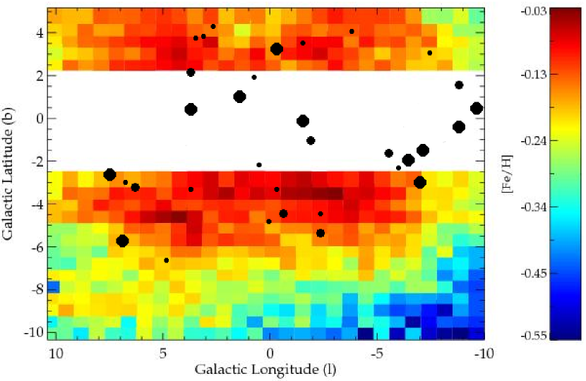
Figure 5: Distribution of the GB sample stars overlayed on the distribution of mean metallicities in the Galactic bulge of Gonzalez et al. (2013). The different symbol sizes mark the members of the low- and high-luminosity group and the stars with luminosities in between.

The metallicity argument can be tested for consistency in comparison with the spatial distribution of the GB sample with the global metallicity distribution in the Galactic bulge. Fig. 5 shows the metallicity map of Gonzalez et al. (2013), which clearly confirms the vertical metallicity gradient with metal-rich stars dominating the inner bulge in regions closer to the Galactic plane ($\mid b\mid<5^{\circ}$). The GB sample members are overplotted. They are completely confined to the more metal rich part of the bulge. Although the mean metallicities in the $30^{\prime}\times 45^{\prime}$ bins of the metallicity map do not reach super-solar metallicities, higher metallicities may occur on smaller spatial scales, where the GB sample members may be located. Therefore, at least this comparison does not contradict the model predictions that the chemistry of intermediate-mass stars at the termination of TP-AGB evolution depends on the metal content of the environment in which they were born.

4.4 The low-luminosity group

Almost half of the sample has luminosities L $<$ 7000 L_⊙ (log L $<$ 3.85) and mass-loss rates (1 – 5) $\times$$10^{-5}$ M_⊙ yr^-1. These kinds of combinations of relatively low luminosities and very high mass-loss rates are not predicted by the models either, at least as long the stars are considered to be on the TP-AGB and in between two thermal pulses (the interpulse phase). Assuming that the stars are in the final phase of their AGB evolution (the last couple of interpulse periods) and making the requirement that the luminosities do not surpass 7000 L_⊙, these stars must have descended from 1.1 $\la$ M_MS $\la$ 1.8 M_⊙ main-sequence stars (Fig. 4).

In models of TP-AGB evolution, mass-loss rates exceeding $10^{-7}$ M_⊙ are not assumed to occur before large amplitude pulsations of the stellar envelope have been established. Most members of the GB sample have not been monitored for variability, except the few sources in common with van der Veen & Habing (1990), for which they report large amplitude variability with periods P$>750$ days. The other sources usually have high IRAS variability index ($>95$, see Table 1), indicating that they are also, in the majority, large amplitude variable stars. We therefore exclude the remote possibility that the members of the low-luminosity group are intermediate-mass stars (M_MS ¿ 3.0 M_⊙) on the early AGB preceding the TP-AGB, although the observed luminosities (L $<$ 7000 L_⊙) are achieved by models during this phase (Bertelli et al., 2008).

During the TP-AGB, the mass-loss rates steadily increase, modulated by the intervening thermal pulses, which affect the surface luminosity and radius of the stars. During the interpulse phase, the stellar luminosity reaches its maximum shortly before the next thermal pulse happens and is referred here to as quiescent luminosity. The models of Vassiliadis & Wood (1993) provide the mass-loss rates ($>$ $10^{-5}$ M_⊙ yr^-1) observed for M_MS $>$ 2.0 M_⊙ during the last couple of interpulse periods, but the correspondent model luminosities are too high. Blöcker (1995) presents models with M_MS = 1, 3, 4, 5, and 7 M_⊙. While the 1 M_⊙ model does not reach the TP-AGB phase, the M_MS = 3 M_⊙ model has quiescent luminosities in the required range, but does not reach mass-loss rates surpassing $10^{-5}$ M_⊙ yr^-1. Models for larger masses do reach the required mass-loss rates, but are again too luminous. Marigo & Girardi (2007) and Weiss & Ferguson (2009) also arrive at the same result: the high observed mass-loss rates are not predicted for the mass ranges corresponding to the observed quiescent luminosities. Given the short times the thermal pulses last ($\sim$ several hundred years, Vassiliadis & Wood 1993), it is unlikely that all these stars are currently experiencing a boost of the mass-loss rate following the brief increases of the luminosity.

A possible explanation for the discrepancies between the observed properties and the model predictions may originate in the assumptions concerning the relation between mass-loss rates and other properties in the TP-AGB models. As no complete mass-loss theory for AGB stars is available, mass-loss rates are empirically coupled to pulsational period. The periods are theoretically determined from relations involving mass and radius, which are provided by the models. While these relations provide resonable values in general, there might be brief phases where the predictions are insufficient. At least for the low luminosity part of our sample, which had main-sequence masses M_MS $<$ 2 M_⊙, the models predict mass-loss rates that are too low in the brief final evolutionary phase.

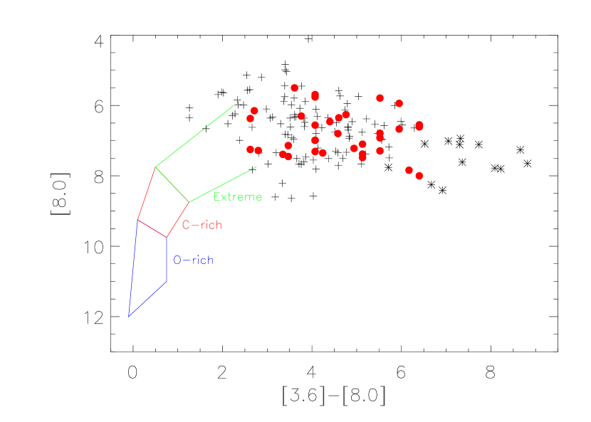
Figure 6: Location of the GB sample stars (red filled circles) in the [3.6]–[8.0] vs. [8.0] colour-magnitude diagram assuming a distance corresponding to the LMC. The boundaries of the locations of the different type of AGB stars (O-rich, C-rich and extreme) as defined by the SAGE project are taken from Blum et al. (2006). In addition, the ‘evolved stars’ in the LMC (plus signs) identified by Gruendl & Chu (2009), and the spectroscopically confirmed C stars (asterisks) from Gruendl et al. (2008) are overplotted.

4.5 Comparison with the AGB population in the LMC

In the LMC, the AGB population has been studied extensively by the SAGE project (Blum et al., 2006). The chemistry of the population was determined from photometry using basically the J–[3.6] vs. [3.6] colour-magnitude diagram (CMD). In Fig. 6 the boundaries for different chemistries are delineated in the [3.6]–[8.0] vs. [8.0] CMD, which is more appropriate for very obscured stars. While C stars are in general found to be redder than O-rich stars, Blum et al. also define a group of ‘extreme stars’ with even redder colours ($J-[3.6]$ $>$ 3.1 mag), for which the chemistry could not be determined. The few known stars of this group, which have been observed spectroscopically, are predominantly C-rich. Along with the model predictions that the lowest effective temperatures and hence the largest mass-loss rates are achieved when the stars become C-rich, the ‘extreme stars’ are uniformly classified as predominantly C-rich (Srinivasan et al., 2011; Riebel et al., 2012). However, a minority population of O-rich stars is not excluded and contamination with red supergiants and young stellar objects is probably also present (Srinivasan et al., 2009; Blum et al., 2014).

We determined synthetic apparant magnitudes in the [3.6] and [8.0] bands of the GLIMPSE photometric system (Churchwell et al., 2009) for all stars of the GB sample using the DUSTY model fits. Comparison with the actually observed magnitudes by GLIMPSE gives an uncertainty of $\sim$ 1 mag. To compare the location of the sample in the CMD of Blum et al. (2006), a distance modulus of 4.0 mag was used to account for the distance difference between the LMC and the Galactic bulge. As shown in Fig. 6, the GB sample stars are located in a sparsely populated region extending the branch populated by the ‘extreme stars’ towards redder colours $[3.6]-[8.0]$ $>$ 2.5 mag. This region of the CMD was also found by Gruendl & Chu (2009) to be populated by ‘evolved stars’. The reddest of them (dubbed EROS for ‘Extremely Red ObjectS’) were spectroscopically observed by Gruendl et al. (2008), showing C-rich chemistry. It follows that while the SAGE ‘extreme stars’ and the even redder ‘evolved stars’ of Gruendl & Chu (2009) in the LMC are predominantly C-rich, the corresponding population in the Galactic bulge represented by the GB sample seem to be O-rich.

Riebel et al. (2012) determined dust mass-loss rates for the SAGE stars using model SEDs. Almost all ‘extreme stars’ were matched with C-rich models. Most dust mass-loss rates for O-rich stars are in the range $10^{-11}$ – $10^{-9}$ M_⊙ yr^-1, and for C-rich stars $>$ $10^{-10}$ M_⊙ yr^-1. With a gas-to-dust ratio of $\sim$ 200 their total mass-loss rates are well below the rates achieved during the superwind. The separation of O-rich and C-rich sources in the SAGE CMDs is very likely valid only as long as mass-loss rates are low, the CSEs are optically thin and therefore the stellar temperature is able to influence the infrared colours. As soon as the mass-loss rates increase, and especially during superwind phases, the stars migrate in CMDs towards redder colours, independent of their current chemistry. Gruendl et al. (2008) find a mean luminosity of 7100 L_⊙ for their EROS sources, and conclude that these stars must have descended from 1.5 – 2.5 M_⊙ main-sequence stars. The total mass-loss rates derived are in the range of (4 – 23) $\times$ $10^{-5}$ M_⊙ yr^-1, much larger than derived for the SAGE AGB stars. The EROS luminosities, main-sequence masses, and mass-loss rates are in perfect agreement with those derived here for the GB sample. The main difference is the chemical composition. As we previously concluded for the GB sample, Gruendl et al. (2008) noted that the mass-loss rates of the EROS sources typically exceed the maximum expected for both O-rich and C-rich AGB stars with luminosities in the observed range.

5 Conclusions

The reddest bright 25 $\mu$m sources towards the Galactic bulge with IRAS colours expected for AGB stars were found to span a luminosity range from $\sim$ 3000 to $\sim$ 30,000 L_⊙ and mass-loss rates between $\sim$ $10^{-5}$ – 3 $\times$ $10^{-4}$ M_⊙ yr^-1. For the lower luminosity group with L $<$ 7000 L_⊙ the main-sequence progenitor masses are in the range 1.1 – 1.8 M_⊙, assuming solar metallicity. With mass-loss rates (1 – 5) $\times$ $10^{-5}$ M_⊙ yr^-1 their stellar envelopes are lost in mere 10,000 – 200,000 years and AGB evolution is terminated. One concludes that the heavily obscured AGB stars do not necessarily descend from massive AGB stars (M_MS $>$ 4 M_⊙) only. At higher luminosities (10,000 – 25,000 L_⊙), AGB evolutionary models predict that for metallicities similar to the Sun or less these high-mass loss stars should already be converted to C-rich chemistry. On the contrary, in the bulge these stars are mostly O-rich. The models predict that the conversion to C-rich chemistry can be delayed or inhibited for higher than solar metallicities. Our sources might have been born in regions of the bulge, where several generations of stars have leftover processed matter with higher than solar metallicity. Their spatial distribution favourably coincides with regions of higher mean metallicities in the Galactic bulge.

Figure 7: Observation and model fits after correcting for interstellar extinction. 2MASS: circles; VVV-DR1: stars; WISE: triangles pointing up; GLIMPSE: sails; MSX: squares; AKARI: diamonds; IRAS: crosses; Upper limits: filled triangles pointing down; Unconfirmed detection: open triangles pointing down; Model: solid line (in case of two models, the solid line represents the brighter and the pointed line the fainter phase (see Section 3.2)).

Figure 7: continued.

Figure 7: continued.

Figure 7: continued.

Figure 7: continued.

Figure 7: continued.

Figure 7: continued.

Figure 7: continued.

Figure 7: continued.

Figure 7: continued.