DuQuad: an inexact (augmented) dual first order algorithm for quadratic programming

Abstract

In this paper we present the solver DuQuad specialized for solving general convex quadratic problems arising in many engineering applications. When it is difficult to project on the primal feasible set, we use the (augmented) Lagrangian relaxation to handle the complicated constraints and then, we apply dual first order algorithms based on inexact dual gradient information for solving the corresponding dual problem. The iteration complexity analysis is based on two types of approximate primal solutions: the primal last iterate and an average of primal iterates. We provide computational complexity estimates on the primal suboptimality and feasibility violation of the generated approximate primal solutions. Then, these algorithms are implemented in the programming language C in DuQuad, and optimized for low iteration complexity and low memory footprint. DuQuad has a dynamic Matlab interface which make the process of testing, comparing, and analyzing the algorithms simple. The algorithms are implemented using only basic arithmetic and logical operations and are suitable to run on low cost hardware. It is shown that if an approximate solution is sufficient for a given application, there exists problems where some of the implemented algorithms obtain the solution faster than state-of-the-art commercial solvers.

1 Introduction

Nowadays, many engineering applications can be posed as convex quadratic problems (QP). Several important applications that can be modeled in this framework such us model predictive control for a dynamical linear system DomZgr:12 ; NecNed:13 ; NedNec:12 ; PatBem:12 ; StaSzu:14 and its dual called moving horizon estimation FraVuk:14 , DC optimal power flow problem for a power system ZimMur:11 , linear inverse problems arising in many branches of science BecTeb:09 ; WanLin:13 or network utility maximization problems WeiOzd:10 have attracted great attention lately. Since the computational power has increased by many orders in the last decade, highly efficient and reliable numerical optimization algorithms have been developed for solving the optimization problems arising from these applications in very short time. For example, these hardware and numerical recent advances made it possible to solve linear predictive control problems of nontrivial sizes within the range of microseconds and even on hardware platforms with limited computational power and memory JerLin:12 .

The theoretical foundation of quadratic programming dates back to the work by Frank & Wolfe FraWol:56 . After the publication of the paper FraWol:56 many numerical algorithms have been developed in the literature that exploit efficiently the structure arising in this class of problems. Basically, we can identify three popular classes of algorithms to solve quadratic programs: active set methods, interior point methods and (dual) first order methods.

Active set methods are based on the observation that quadratic problems with equality constraints are equivalent to solving a linear system. Thus, the iterations in these methods are based on solving a linear system and updating the active set (the term active set refers to the subset of constraints that are satisfied as equalities by the current estimate of the solution). Active set general purpose solvers are adequate for small-to-medium scale quadratic problems, since the numerical complexity per iteration is cubic in the dimension of the problem. Matlab’s quadprog function implements a primal active set method. Dual active set methods are available in the codes BarBie:06 ; FerKir:14 .

Interior point methods remove the inequality constraints from the problem formulation using a barrier term in the objective function for penalizing the constraint violations. Usually a logarithmic barrier terms is used and the resulting equality constrained nonlinear convex problem is solved by the Newton method. Since the iteration complexity grows also cubically with the dimension, interior-point solvers are also the standard for small-to-medium scale QPs. However, structure exploiting interior point solvers have been also developed for particular large-scale applications: e.g. several solvers exploit the sparse structure of the quadratic problem arising in predictive control (CVXGEN MatBoy:09 , FORCES DomZgr:12 ). A parallel interior point code that exploits special structures in the Hessian of large-scale structured quadratic programs have been developed in GonGro:07 .

First order methods use only gradient information at each iterate by computing a step towards the solution of the unconstrained problem and then projecting this step onto the feasible set. Augmented Lagrangian algorithms for solving general nonconvex problems are presented in the software package Lancelot ConGou:92 . For convex QPs with simple constraints we can use primal first order methods for solving the quadratic program as in Ulm:11 . In this case the main computational effort per iteration consists of a matrix-vector product. When the projection on the primal feasible set is hard to compute, an alternative to primal first order methods is to use the Lagrangian relaxation to handle the complicated constraints and then to apply dual first order algorithms for solving the dual. The computational complexity certification of first order methods for solving the (augmented) Lagrangian dual of general convex problems is studied e.g. in LanMon:08 ; NecNed:13 ; NedNec:12 ; NecFer:15 ; NedOzd:09 and of quadratic problems is studied in Gis:14 ; PatBem:12 ; StaSzu:14 . In these methods the main computational effort consists of solving at each iteration a Lagrangian QP problem with simple constraints for a given multiplier, which allows us to determine the value of the dual gradient for that multiplier, and then update the dual variables using matrix-vector products. For example, the toolbox FiOrdOs Ulm:11 auto-generates code for primal or dual fast gradient methods as proposed in RicMor:11 . The algorithm in PatBem:12 dualizes only the inequality constraints of the QP and assumes available a solver for linear systems that is able to solve the Lagrangian inner problem. However, both implementations Ulm:11 ; PatBem:12 do not consider the important aspect that the Lagrangian inner problem cannot be solved exactly in practice. The effect of inexact computations in dual gradient values on the convergence of dual first order methods has been analyzed in detail in NecNed:13 ; NedNec:12 ; NecFer:15 . Moreover, most of these papers generate approximate primal solutions through averaging NecNed:13 ; NedNec:12 ; NedOzd:09 . On the other hand, in practice usually the last primal iterate is employed, since in practice these methods converge faster in the primal last iterate than in a primal average sequence. These issues motivate our work here.

Contributions. In this paper we analyze the computational complexity of several (augmented) dual first order methods implemented in DuQuad for solving convex quadratic problems. Contrary to most of the results from the literature NedOzd:09 ; PatBem:12 , our approach allows us to use inexact dual gradient information (i.e. it allows to solve the (augmented) Lagrangian inner problem approximately) and therefore is able to tackle more general quadratic convex problems and to solve practical applications. Another important feature of our approach is that we provide also complexity results for the primal latest iterate, while in much of the previous literature convergence rates in an average of primal iterates are given NecNed:13 ; NedNec:12 ; NedOzd:09 ; PatBem:12 . We derive in a unified framework the computational complexity of the dual and augmented dual (fast) gradient methods in terms of primal suboptimality and feasibility violation using inexact dual gradients and two types of approximate primal solutions: the last primal iterate and an average of primal iterates. From our knowledge this paper is the first where both approaches, dual and augmented dual first order methods, are analyzed uniformly. These algorithms are also implemented in the efficient programming language C in DuQuad, and optimized for low iteration complexity and low memory footprint. The toolbox has a dynamic Matlab interface which make the process of testing, comparing, and analyzing the algorithms simple. The algorithms are implemented using only basic arithmetic and logical operations and thus are suitable to run on low cost hardware. The main computational bottleneck in the methods implemented in DuQuad is the matrix-vector product. Therefore, this toolbox can be used for solving either QPs on hardware with limited resources or sparse QPs with large dimension.

Contents. The paper is organized as follows. In section 2 we describe the optimization problem that we solve in DuQuad. In Section 3 we describe the the main theoretical aspects that DuQuad is based on, while in Section 6 we present some numerical results obtained with DuQuad.

Notation. For $x,y\in\mathbb{R}^{n}$ denote the scalar product by $\langle x,y\rangle=x^{T}y$ and the Euclidean norm by $\|x\|=\sqrt{x^{T}x}$. Further, $[u]_{X}$ denotes the projection of $u$ onto convex set $X$ and $\text{dist}_{X}(u)=\|u-[u]_{X}\|$ its distance. For a matrix $G\in\mathbb{R}^{m\times n}$ we use the notation $\|G\|$ for the spectral norm.

2 Problem formulation

In DuQuad we consider a general convex quadratic problem (QP) in the form:

$$F^{*}= \min_{u\in U}F(u)\quad\left(=\frac{1}{2}u^{T}Qu+q^{T}u\right)$$ (1)

$$\text{s.t:}\;\;\;Gu+g\in\mathcal{K},$$

where $F:\mathbb{R}^{n}\rightarrow\mathbb{R}$ is a convex quadratic function with the Hessian $Q\succeq 0$, $G\in\mathbb{R}^{p\times n}$, $U\subseteq\mathbb{R}^{n}$ is a simple compact convex set, i.e. a box $U=[\text{lb}\;\text{ub}]$, and ${\mathcal{K}}$ is either the cone $\mathbb{R}^{p}_{-}$ or the cone $\{0\}$. Note that our formulation allows to incorporate in the QP either linear inequality constraints $\mathcal{K}=\mathbb{R}^{p}_{-}$ (arising e.g. in sparse formulation of predictive control and network utility maximization) or linear equality constraints $\mathcal{K}=\{0\}$ (arising e.g. in condensed formulation of predictive control and DC optimal power flow). In fact the user can define linear constraints of the form: $\bar{\text{lb}}\leq\bar{G}u+\bar{g}\leq\bar{\text{ub}}$ and depending on the values for $\bar{\text{lb}}$ and $\bar{\text{ub}}$ we have linear inequalities or equalities. Throughout the paper we assume that there exists a finite optimal Lagrange multiplier $\lambda^{*}$ for the QP (1) and it is difficult to project on the feasible set of problem (1):

$${\cal X}_{QP}=\{u\in U:\;Gu+g\in\mathcal{K}\}.$$

Therefore, solving the primal problem (1) approximately with primal first order methods is numerically difficult and thus we usually use (augmented) dual first order methods for finding an approximate solution for (1). By moving the complicating constraints $Gu+g\in\mathcal{K}$ into the cost via Lagrange multipliers we define the (augmented) dual function:

$$d_{\rho}(\lambda)=\min_{u\in U}\mathcal{L}_{\rho}(u,\lambda),$$ (2)

where $\mathcal{L}_{\rho}(u,\lambda)$ denotes the (augmented) Lagrangian w.r.t. the complicating constraints $Gu+g\in\mathcal{K}$, i.e.:

$$\mathcal{L}_{\rho}(u,\lambda)=\min\limits_{s\in\mathcal{K}}\;F(u)+\langle\lambda,Gu+g-s\rangle+\frac{\rho}{2}\lVert Gu+g-s\rVert^{2}$$ (3)

where the regularization parameter $\rho\geq 0$. We denote $s(u,\lambda)=\arg\min\limits_{s\in\mathcal{K}}\langle\lambda,Gu+g-s\rangle+\frac{\rho}{2}\lVert Gu+g-s\rVert^{2}$ and observe that:

$$s(u,\lambda)=\begin{cases}\left[Gu+g+\frac{1}{\rho}\lambda\right]_{\mathcal{K}}&\text{if}\;\;\rho>0\\ 0&\text{if}\;\;\rho=0.\end{cases}$$

Using this observation in the formulation (3), we obtain:

$$\mathcal{L}_{\rho}(u,\lambda)=\begin{cases}F(u)+\frac{\rho}{2}\text{dist}_{\mathcal{K}}\left(Gu+g+\frac{1}{\rho}\lambda\right)^{2}-\frac{1}{2\rho}\lVert\lambda\rVert^{2},&\text{if}\;\rho>0\\ F(u)+\langle\lambda,Gu+g\rangle,&\text{if}\;\rho=0.\end{cases}$$ (4)

In order to tackle general convex quadratic programs, in DuQuad we consider the following two options:

Case 1: if $Q\succ 0$, i.e. $Q$ has the smallest eigenvalue $\lambda_{\min}(Q)>0$, then we consider $\rho=0$ and recover the ordinary Lagrangian function.

Case 2: if $Q\succeq 0$, i.e. $Q$ has the smallest eigenvalue $\lambda_{\min}(Q)=0$, then we consider $\rho>0$ and recover the augmented Lagrangian function.

Our formulation of the (augmented) Lagrangian (4) and the previous two cases allow us to thereat in a unified framework both approaches, dual and augmented dual first order methods, for general convex QPs. We denote by $u(\lambda)$ the optimal solution of the inner problem with simple constraints $u\in U$:

$$u(\lambda)=\arg\min_{u\in U}\mathcal{L}_{\rho}(u,\lambda).$$ (5)

Note that for both cases described above the (augmented) dual function is differentiable everywhere. Moreover, the gradient of the (augmented) dual function $d_{\rho}(\lambda)$ is $L_{\text{d}}$-Lipschitz continuous and given by NecNed:13 ; NedNec:12 ; Nes:04 ; Roc:76 :

$$\nabla d_{\rho}(\lambda)=Gu(\lambda)+g-s(u(\lambda),\lambda)\;\;\text{and}\;\;L_{\text{d}}=\frac{\|G\|^{2}}{\lambda_{\min}(Q)+\rho\|G\|^{2}}$$ (6)

for all $\lambda\in\mathbb{R}^{p}$. Since the dual function has Lipschitz continuous gradient, we can derive bounds on $d_{\rho}$ in terms of a linear and a quadratic model (the so-called descent lemma) Nes:04 :

$$0\leq[d_{\rho}(\mu)+\langle{\nabla}d_{\rho}(\mu),\lambda-\mu\rangle]-d_{\rho}(\lambda)\leq\frac{L_{\text{d}}}{2}\|\mu-\lambda\|^{2}\quad\forall\lambda,\mu\in\mathbb{R}^{p}.$$ (7)

Descent lemma is essential in proving convergence rate for first order methods Nes:04 . Since we assume the existence of a finite optimal Lagrange multiplier for (1), strong duality holds and thus the outer problem is smooth and satisfies:

$$F^{*}=\max_{\lambda\in\mathcal{K}_{d}}d_{\rho}(\lambda),$$ (8)

where

$$\mathcal{K}_{d}=\begin{cases}\mathbb{R}^{p}_{+},&\text{if}\;\;Q\succ 0\;\;\text{and}\;\;\mathcal{K}=\mathbb{R}^{p}_{-}\\ \mathbb{R}^{p},&\;\;\text{otherwise}.\end{cases}$$

Note that, in general, the smooth (augmented) dual problem (8) is not a QP, but has simple constraints. We denote a primal optimal solution by $u^{*}$ and a dual optimal solution by $\lambda^{*}$. We introduce $\Lambda^{*}\subseteq\mathcal{K}_{d}$ as the set of optimal solutions of the smooth dual problem (8) and define for some $\lambda^{0}\in\mathbb{R}^{p}$ the following finite quantity:

$$\mathcal{R}_{\text{d}}=\min\limits_{\lambda^{*}\in\Lambda^{*}}\|\lambda^{*}-\lambda^{0}\|.$$ (9)

In the next section we present a general first order algorithm for convex optimization with simple constraints that is used frequently in our toolbox.

2.1 First order methods

In this section we present a framework for first order methods generating an approximate solution for a smooth convex problem with simple constraints in the form:

$$\phi^{*}=\min_{x\in X}\;\phi(x),$$ (10)

where $\phi:\mathbb{R}^{n}\to\mathbb{R}$ is a convex function and $X$ is a simple convex set (i.e. the projection on this set is easy). Additionally, we assume that $\phi$ has Lipschitz continuous gradient with constant $L_{\phi}>0$ and is strongly convex with constant $\sigma_{\phi}\geq 0$. This general framework covers important particular algorithms Nes:04 ; BecTeb:09 : e.g. gradient algorithm, fast gradient algorithm for smooth problems, or fast gradient algorithm for problems with smooth and strongly convex objective function. Thus, we will analyze the iteration complexity of the following general first order method that updates two sequences $(x^{k},y^{k})_{k\geq 0}$ as follows:

Algorithm FOM ($\phi,X$) Given $x^{0}=y^{1}\in X$, for $k\geq 1$ compute: 1. ${x}^{k}=\left[y^{k}-\frac{1}{L_{\phi}}\nabla\phi(y^{k})\right]_{X}$, 2. $y^{k+1}=x^{k}+\beta_{k}(x^{k}-x^{k-1})$,

where $\beta_{k}$ is the parameter of the method and we choose it in an appropriate way depending on the properties of function $\phi$. More precisely, $\beta_{k}$ can be updated as follows:

GM: in the Gradient Method $\beta_{k}=\frac{\theta_{k}-1}{\theta_{k+1}}$, where $\theta_{k}=1$ for all $k$. This is equivalent with $\beta_{k}=0$ for all $k$. In this case $y^{k+1}=x^{k}$ and thus we have the classical gradient update: ${x}^{k+1}=[x^{k}-\frac{1}{L_{\phi}}\nabla\phi(x^{k})]_{X}$.

FGM: in the Fast Gradient Method for smooth convex problems $\beta_{k}=\frac{\theta_{k}-1}{\theta_{k+1}}$, where $\theta_{k+1}=\frac{1+\sqrt{1+4\theta_{k}^{2}}}{2}$ and $\theta_{1}=1$. In this case we get a particular version of Nesterov’s accelerated scheme Nes:04 that updates two sequences $(x^{k},y^{k})$ and has been analyzed in detail in BecTeb:09 .

FGM_σ: in fast gradient algorithm for smooth convex problems with strongly convex objective function, with constant $\sigma_{\phi}>0$, we choose $\beta_{k}=\frac{\sqrt{L_{\phi}}-\sqrt{\sigma_{\phi}}}{\sqrt{L_{\phi}}+\sqrt{\sigma_{\phi}}}$ for all $k$. In this case we get a particular version of Nesterov’s accelerated scheme Nes:04 that also updates two sequences $(x^{k},y^{k})$.

The convergence rate of Algorithm FOM($\phi,X$) in terms of function values is given in the next lemma:

Lemma 1

BecTeb:09 ; Nes:04 For smooth convex problem (10) assume that the objective function $\phi$ is strongly convex with constant $\sigma_{\phi}\geq 0$ and has Lipschitz continuous gradient with constant $L_{\phi}>0$. Then, the sequences $\left(x^{k},y^{k}\right)_{k\geq 0}$ generated by Algorithm FOM($\phi,X$) satisfy:

$$\phi(x^{k})-\phi^{*}\!\leq\!\min\!\left(\!\!\left(\!1\!-\!\sqrt{\frac{\sigma_{\phi}}{L_{\phi}}}\right)^{k-1}\!\!\!\!\!\!L_{\phi}\mathcal{R}^{2}_{\phi},\frac{2L_{\phi}\mathcal{R}^{2}_{\phi}}{(k\!+\!1)^{p(\beta_{k})}}\!\right)$$ (11)

where $\mathcal{R}_{\phi}=\min\limits_{x^{*}_{\phi}\in X^{*}_{\phi}}\|x^{0}-x^{*}_{\phi}\|$, with $X^{*}_{\phi}$ the optimal set of (10), and $p(\beta_{k})$ is defined as follows:

$$p(\beta_{k})=\begin{cases}1&\mbox{if }\beta_{k}=0\\ 2&\mbox{otherwise}.\end{cases}$$ (12)

Thus, Algorithm FOM has linear convergence provided that $\sigma_{\phi}>0$. Otherwise, it has sublinear convergence.

3 Inexact (augmented) dual first order methods

In this section we describe an inexact dual (augmented) first order framework implemented in DuQuad, a solver able to find an approximate solution for the quadratic program (1). For a given accuracy $\epsilon>0$, $u_{\epsilon}\in U$ is called an $\epsilon$-primal solution for problem (1) if the following inequalities hold:

$$\text{dist}_{\mathcal{K}}(Gu_{\epsilon}+g)\leq{\cal O}(\epsilon)\quad\text{and}\quad|F(u_{\epsilon})-F^{*}|\leq{\cal O}(\epsilon).$$

The main function in DuQuad is the one implementing the general Algorithm FOM. Note that if the feasible set ${\cal X}_{QP}$ of (1) is simple, then we can call directly FOM($F,{\cal X}_{QP}$) in order to obtain an approximate solution for (1). However, in general the projection on ${\cal X}_{QP}$ is as difficult as solving the original problem. In this case we resort to the (augmented) dual formulation (8) for finding an $\epsilon$-primal solution for the original QP (1). The main idea in DuQuad is based on the following observation: from (5)–(6) we observe that for computing the gradient value of the dual function in some multiplier $\lambda$, we need to solve exactly the inner problem (5); despite the fact that, in some cases, the (augmented) Lagrangian $\mathcal{L}_{\rho}(u,\lambda)$ is quadratic and the feasible set $U$ is simple in (5), this inner problem generally cannot be solved exactly. Therefore, the main iteration in DuQuad consists of two steps:

Step 1: for a given inner accuracy $\epsilon_{\text{in}}$ and a multiplier $\mu\in\mathbb{R}^{p}$ solve approximately the inner problem (5) with accuracy $\epsilon_{\text{in}}$ to obtain an approximate solution $\bar{u}(\mu)$ instead of the exact solution $u(\mu)$, i.e.:

$$0\leq\mathcal{L}_{\rho}(\bar{u}(\mu),\mu)-d_{\rho}(\mu)\leq\epsilon_{\text{in}}.$$ (13)

In DuQuad, we obtain an approximate solution $\bar{u}(\mu)$ using the Algorithm FOM($\mathcal{L}_{\rho}(\cdot,\mu),U$). From, Lemma 1 we can estimate tightly the number of iterations that we need to perform in order to get an $\epsilon_{\text{in}}$-solution $\bar{u}(\mu)$ for (5): the Lipschitz constant is $L_{\mathcal{L}}=\lambda_{\max}(Q)+\rho\|G\|^{2}$, the strong convexity constant is $\sigma_{\mathcal{L}}=\lambda_{\min}(Q+\rho G^{T}G)$ (provided that e.g. $\mathcal{K}=\{0\}$) and ${\cal R}_{\mathcal{L}}\leq D_{U}$ (the diameter of the box set $U$). Then, the number of iterations that we need to perform for computing $\bar{u}(\mu)$ satisfying (13) can be obtained from (11).

Step 2: Once an $\epsilon_{\text{in}}$-solution $\bar{u}(\mu)$ for (5) was found, we update at the outer stage the Lagrange multipliers using again Algorithm FOM($d_{\rho},{\mathcal{K}}_{d}$). Note that for updating the Lagrange multipliers we use instead of the true value of the dual gradient $\nabla d_{\rho}(\mu)=Gu(\mu)+g-s(u(\mu),\mu)$, an approximate value given by: $\bar{\nabla}d_{\rho}(\mu)=G\bar{u}(\mu)+g-s(\bar{u}(\mu),\mu)$.

In DevGli:14 ; NedNec:12 ; NecNed:13 ; NecFer:15 it has been proved separately, for dual and augmented dual first order methods, that using an appropriate value for $\epsilon_{\text{in}}$ (depending on the desired accuracy $\epsilon$ that we want to solve the QP (1)) we can still preserve the convergence rates of Algorithm FOM($d_{\rho},{\mathcal{K}}_{d}$) given in Lemma 1, although we use inexact dual gradients. In the sequel, we derive in a unified framework the computational complexity of the dual and augmented dual (fast) gradient methods. From our knowledge, this is the first time when both approaches, dual and augmented dual first order methods, are analyzed uniformly. First, we show that by introducing inexact values for the dual function and for its gradient given by the following expressions:

$$\bar{d}_{\rho}(\mu)=\mathcal{L}_{\rho}(\bar{u}(\mu),\mu)\;\;\text{and}\;\;\bar{\nabla}d_{\rho}(\mu)=G\bar{u}(\mu)+g-s(\bar{u}(\mu),\mu),$$ (14)

then we have a similar descent relation as in (7) given in the following lemma:

Lemma 2

Given $\epsilon_{\text{in}}>0$ such that (13) holds, then based on the definitions (14) we get the following inequalities:

$$0\leq[\bar{d}_{\rho}(\mu)\!+\langle\bar{\nabla}d_{\rho}(\mu),\lambda-\mu\rangle]-d_{\rho}(\lambda)\leq\!L_{\text{d}}\|\mu-\lambda\|^{2}+\!2\epsilon_{\text{in}}\quad\forall\lambda,\mu\!\in\!\mathbb{R}^{p}.$$ (15)

Proof

From the definition of $d_{\rho}$, (13) and (14) it can be derived:

$$d_{\rho}(\lambda) =\min\limits_{u\in U,\;s\in\mathcal{K}}F(u)+\langle\lambda,Gu+g-s\rangle+\frac{\rho}{2}\lVert Gu+g-s\rVert^{2}$$

$$\leq F(\bar{u}(\mu))+\left\langle\lambda,G\bar{u}(\mu)+g-s(\bar{u}(\mu),\mu)\right\rangle+\frac{\rho}{2}\left\|G\bar{u}(\mu)+g-s(\bar{u}(\mu),\mu)\right\|^{2}$$

$$=\mathcal{L}_{\rho}(\bar{u}(\mu),\mu)+\langle G\bar{u}(\mu)+g-s(\bar{u}(\mu),\mu),\lambda-\mu\rangle$$

$$=\bar{d}_{\rho}(\mu)+\langle\bar{\nabla}d_{\rho}(\mu),\lambda-\mu\rangle,$$

which proves the first inequality. In order to prove the second inequality, let $\tilde{u}\in U$ be a fixed primal point such that $\mathcal{L}_{\rho}(\tilde{u},\mu)\geq d_{\rho}(\mu)$. Then, we note that the nonnegative function $h(\mu)=\mathcal{L}_{\rho}(\tilde{u},\mu)-d_{\rho}(\mu)\geq 0$ has Lipschitz gradient with constant $L_{d}$ and thus we have Nes:04 :

$$\frac{1}{2L_{d}} \left\|\left(G\tilde{u}+g-s(\tilde{u},\mu)\right)-\nabla d_{\rho}(\mu)\right\|^{2}=\frac{1}{2L_{d}}\lVert\nabla h(\mu)\rVert^{2}$$

$$\leq h(\mu)-\min_{\nu\in\mathbb{R}^{p}}h(\nu)\leq\mathcal{L}_{\rho}(\tilde{u},\mu)-d_{\rho}(\mu).$$

Taking now $\tilde{u}=\bar{u}(\mu)$ and using (13), then we obtain:

$$\lVert\bar{\nabla}d_{\rho}(\mu)-\nabla d_{\rho}(\mu)\rVert\leq\sqrt{2L_{d}\epsilon_{\text{in}}}\qquad\forall\mu\in\mathbb{R}^{p}.$$ (16)

Furthermore, combining (16) with (7) and (13) we have:

$$d_{\rho}(\lambda)\geq\bar{d}_{\rho}(\mu)+\langle\nabla d_{\rho}(\mu),\lambda-\mu\rangle-\frac{L_{d}}{2}\lVert\lambda-\mu\rVert^{2}-\epsilon_{\text{in}}$$

$$\geq\bar{d}_{\rho}(\mu)+\langle\bar{\nabla}d_{\rho}(\mu),\lambda-\mu\rangle-\frac{L_{d}}{2}\lVert\lambda-\mu\rVert^{2}+\langle\nabla d_{\rho}(\mu)-\bar{\nabla}d_{\rho}(\mu),\lambda-\mu\rangle-\epsilon_{\text{in}}$$

$$\geq\bar{d}_{\rho}(\mu)\!+\!\langle\bar{\nabla}d_{\rho}(\mu),\lambda-\mu\rangle-\frac{L_{d}}{2}\lVert\lambda-\mu\rVert^{2}-\lVert\bar{\nabla}d_{\rho}(\mu)\!-\!\nabla d_{\rho}(\mu)\rVert\lVert\lambda-\mu\rVert-\epsilon_{\text{in}}$$

$$\overset{\eqref{inexact_gradient_rel}}{\geq}\bar{d}_{\rho}(\mu)+\langle\bar{\nabla}d_{\rho}(\mu),\lambda-\mu\rangle-\frac{L_{d}}{2}\lVert\lambda-\mu\rVert^{2}-\sqrt{2L_{d}\epsilon_{\text{in}}}\lVert\lambda-\mu\rVert-\epsilon_{\text{in}}.$$

Using the relation $\sqrt{ab}\leq(a+b)/2$ we have:

$$d_{\rho}(\lambda)\geq\bar{d}_{\rho}(\mu)+\langle\bar{\nabla}d_{\rho}(\mu),\lambda-\mu\rangle-L_{d}\lVert\lambda-\mu\rVert^{2}-2\epsilon_{\text{in}},$$

which shows the second inequality of our lemma. ∎

This lemma will play a major role in proving rate of convergence for the methods presented in this paper. Note that in (15) $\epsilon_{\text{in}}$ enters linearly, while in DevGli:14 ; NedNec:12 $\epsilon_{\text{in}}$ enters quadratically in the context of augmented Lagrangian and thus in the sequel we will get better convergence estimates than those in the previous papers. In conclusion, for solving the dual problem (8) in DuQuad we use the following inexact (augmented) dual first order algorithm:

Algorithm DFOM ($d_{\rho},\mathcal{K}_{d}$) Given $\lambda^{0}=\mu^{1}\in\mathcal{K}_{d}$, for $k\geq 1$ compute: 1. $\bar{u}^{k}$ satisfying (13) for $\mu=\mu^{k}$, i.e. $\bar{u}^{k}=\bar{u}(\mu^{k})$ 2. ${\lambda}^{k}=\left[\mu^{k}+\frac{1}{2L_{\text{d}}}\bar{\nabla}d_{\rho}(\mu^{k})\right]_{\mathcal{K}_{d}}$, 3. $\mu^{k+1}=\lambda^{k}+\beta_{k}(\lambda^{k}-\lambda^{k-1})$.

Recall that $\bar{u}^{k}=\bar{u}(\mu^{k})$ satisfying the inner criterion (13) and $\bar{\nabla}d_{\rho}(\mu^{k})=G\bar{u}^{k}+g-s(\bar{u}^{k},\mu^{k})$. Moreover, $\beta_{k}$ is chosen as follows:

• DGM: in (augmented) Dual Gradient Method $\beta_{k}=\frac{\theta_{k}-1}{\theta_{k+1}}$, where $\theta_{k}=1$ for all $k$, or equivalently $\beta_{k}=0$ for all $k$, i.e. the ordinary gradient algorithm.

• DFGM: in (augmented) Dual Fast Gradient Method $\beta_{k}=\frac{\theta_{k}-1}{\theta_{k+1}}$, where $\theta_{k+1}=\frac{1+\sqrt{1+4\theta_{k}^{2}}}{2}$ and $\theta_{1}=1$, i.e. a variant of Nesterov’s accelerated scheme.

Therefore, in DuQuad we can solve the smooth (augmented) dual problem (8) either with dual gradient method DGM ($\beta_{k}=0$) or with dual fast gradient method DFGM ($\beta_{k}$ is updated based on $\theta_{k}$). Recall that for computing $\bar{u}^{k}$ in DuQuad we use Algorithm FOM($\mathcal{L}_{\rho}(\cdot,\mu^{k}),U$) (see the discussion of Step 1). When applied to inner subproblem (5), Algorithm FOM($\mathcal{L}_{\rho}(\cdot,\mu^{k}),U$) will converge linearly provided that $\sigma_{\mathcal{L}}>0$. Moreover, when applying Algorithm FOM($\mathcal{L}_{\rho}(\cdot,\mu^{k}),U$) we use warm start: i.e. we start our iteration from previous computed $\bar{u}^{k-1}$. Combining the inexact descent relation (15) with Lemma 1 we obtain the following convergence rate for the general Algorithm DFOM($d_{\rho},\mathcal{K}_{d}$) in terms of dual function values of (8):

Theorem 3.1

DevGli:14 ; NedNec:12 ; NecNed:13 For the smooth (augmented) dual problem (8) the dual sequences $\left(\lambda^{k},\mu^{k}\right)_{k\geq 0}$ generated by Algorithm DFOM($d_{\rho},\mathcal{K}_{d}$) satisfy the following convergence estimate on dual suboptimality:

$$F^{*}-d_{\rho}(\lambda^{k})\leq\frac{4L_{\text{d}}\mathcal{R}^{2}_{\text{d}}}{(k+1)^{p(\beta_{k})}}+2(k+1)^{p(\beta_{k})-1}\epsilon_{\text{in}},$$ (17)

where recall $\mathcal{R}_{\text{d}}=\min\limits_{\lambda^{*}\in\Lambda^{*}}\|\lambda^{*}-\lambda^{0}\|$ and $p(\beta_{k})$ is defined as in (12). ∎

Note that in (DevGli:14, , Theorem 2), the convergence rate of DGM scheme is provided in the average dual iterate $\hat{\lambda}^{k}=\frac{1}{k+1}\sum\limits_{j=0}^{k}\lambda^{j}$ and not in the last dual iterate $\lambda^{k}$. However, for a uniform treatment in Theorem 3.1 we redefine the dual final point (the dual last iterate $\lambda^{k}$ when some stopping criterion is satisfied) as follows: $\lambda^{k}=\left[\hat{\lambda}^{k}+\frac{1}{2L_{\text{d}}}\bar{\nabla}d_{\rho}(\hat{\lambda}^{k})\right]_{\mathcal{K}_{d}}$.

3.1 How to choose inner accuracy $\epsilon_{\text{in}}$ in DuQuad

We now show how to choose the inner accuracy $\epsilon_{\text{in}}$ in DuQuad. From Theorem 3.1 we conclude that in order to get $\epsilon$-dual suboptimality, i.e. $F^{*}-d_{\rho}(\lambda^{k})\leq\epsilon$, the inner accuracy $\epsilon_{\text{in}}$ and the number of outer iteration $k_{\text{out}}$ (i.e. number of updates of Lagrange multipliers) have to be chosen as follows:

$$\epsilon_{\text{in}}=\begin{cases}\frac{\epsilon}{4}&\mbox{if }\;\;\textbf{DGM}\\ \frac{\epsilon\sqrt{\epsilon}}{8\mathcal{R}_{\text{d}}\sqrt{2L_{\text{d}}}}&\mbox{if }\;\;\textbf{DFGM},\end{cases}\hskip 20.0ptk_{\text{out}}=\begin{cases}\frac{8L_{d}\mathcal{R}_{d}^{2}}{\epsilon}&\text{if}\;\;\textbf{DGM}\\ \sqrt{\frac{8L_{d}\mathcal{R}_{d}^{2}}{\epsilon}}&\text{if}\;\;\textbf{DFGM}.\end{cases}$$ (18)

Indeed, by enforcing each term of the right hand side of (17) to be smaller than $\frac{\epsilon}{2}$ we obtain first the bound on the number of the outer iterations $k_{\text{out}}$. By replacing this bound into the expression of $\epsilon_{\text{in}}$, we also obtain how to choose $\epsilon_{\text{in}}$, i.e the estimates (18). We conclude that the inner QP (5) has to be solved with higher accuracy in dual fast gradient algorithm DFGM than in dual gradient algorithm DGM. This shows that dual gradient algorithm DGM is robust to inexact (augmented) dual first order information, while dual fast gradient algorithm DFGM is sensitive to inexact computations (see also Fig. 1). In DuQuad the user can choose either Algorithm DFGM or Algorithm DGM for solving the (augmented) dual problem (8) and he can also choose the inner accuracy $\epsilon_{\text{in}}$ for solving the inner problem (in the toolbox the default values for $\epsilon_{\text{in}}$ are taken of the same order as in (18)).

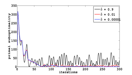
Figure 1: Behavior of Algorithms DGM (left), DFGM(right) in terms of primal suboptimality w.r.t. inner accuracy $\epsilon_{\text{in}}$ for a strongly convex QP with $\epsilon=0.01$.

4 How to recover an $\epsilon$-primal solution in DuQuad

It is natural to investigate how to recover an $\epsilon$-primal solution for the original QP (1). Since dual suboptimality is given in the last dual iterate $\lambda^{k}$, it is natural to consider as an approximate primal solution the last primal iterate generated by Algorithm DFOM in $\lambda^{k}$, i.e.:

$$\bar{u}_{\epsilon}^{k}=\bar{u}(\lambda^{k}).$$ (19)

Note that the last primal iterate $\bar{u}_{\epsilon}^{k}=\bar{u}(\lambda^{k})$ coincides with $\bar{u}^{k}=\bar{u}(\mu^{k})$ for Algorithm DGM. However, for Algorithm DFGM these two sequences are different, i.e. $\bar{u}_{\epsilon}^{k}\not=\bar{u}^{k}$. We will show below that the last primal iterate $\bar{u}_{\epsilon}^{k}$ is an $\sqrt{\epsilon}$-primal solution for the original QP (1), provided that $F^{*}-d_{\rho}(\lambda^{k})\leq\epsilon$. We can also construct an approximate primal solution based on an average of all previous primal iterates generated by Algorithm DFOM , i.e.:

$$\hat{u}_{\epsilon}^{k}=\sum_{j=1}^{k}\frac{\theta_{j}\bar{u}^{j}}{S_{k}},\quad S_{k}=\sum_{j=1}^{k}\theta_{j}.$$ (20)

Recall that $\theta_{j}=1$ in Algorithm DGM and $\theta_{j}$ is updated according to the rule $\theta_{j+1}=\frac{1+\sqrt{1+4\theta_{j}^{2}}}{2}$ and $\theta_{1}=1$ in Algorithm DFGM. In the sequel, we prove that the average of primal iterates sequence $\hat{u}_{\epsilon}^{k}$ is an $\epsilon$-primal solution for the original QP (1), provided that $F^{*}-d_{\rho}(\lambda^{k})\leq\epsilon$.

Before proving primal rate of convergence for Algorithm DFOM we derive a bound on $\lVert\lambda^{k+1}-\lambda^{*}\rVert$, with $\lambda^{k}$ generated by algorithm DFOM, bound that will be used in the proofs of our convergence results. In the case of DGM, using its particular iteration, for any $\lambda\in\mathcal{K}_{d}$, we have:

$$\lVert\lambda^{k+1}-\lambda\rVert^{2} =\lVert\lambda^{k}-\lambda\rVert^{2}+2\langle\lambda^{k+1}-\lambda^{k},\lambda^{k}-\lambda\rangle+\lVert\lambda^{k+1}-\lambda^{k}\rVert^{2}$$

$$=\lVert\lambda^{k}-\lambda\rVert^{2}+2\langle\lambda^{k+1}-\lambda^{k},\lambda^{k+1}-\lambda\rangle-\lVert\lambda^{k+1}-\lambda^{k}\rVert^{2}$$

$$\leq\lVert\lambda^{k}-\lambda\rVert^{2}+\frac{1}{L_{\text{d}}}\langle\bar{\nabla}d_{\rho}(\lambda^{k}),\lambda^{k+1}-\lambda\rangle-\lVert\lambda^{k+1}-\lambda^{k}\rVert^{2}$$

$$=\lVert\lambda^{k}-\lambda\rVert^{2}+\frac{1}{L_{\text{d}}}\langle\bar{\nabla}d_{\rho}(\lambda^{k}),\lambda^{k}-\lambda\rangle$$ (21)

$$\quad\quad+\frac{1}{L_{\text{d}}}\left(\langle\bar{\nabla}d_{\rho}(\lambda^{k}),\lambda^{k+1}-\lambda^{k}\rangle-L_{\text{d}}\lVert\lambda^{k+1}-\lambda^{k}\rVert^{2}\right)$$

$$\leq\lVert\lambda^{k}-\lambda\rVert^{2}+\frac{1}{L_{\text{d}}}(d_{\rho}(\lambda^{k+1})-d_{\rho}(\lambda))+\frac{\epsilon_{\text{in}}}{L_{\text{d}}}.$$

Taking now $\lambda=\lambda^{*}$ and using an inductive argument, we get:

$$\lVert\lambda^{k}-\lambda^{*}\rVert\leq R_{d}+\sqrt{\frac{k\epsilon_{\text{in}}}{L_{\text{d}}}}.$$ (22)

On the other hand, for the scheme DFGM, we introduce the notation $l^{k}=\lambda^{k-1}+\theta_{k}(\lambda^{k}-\lambda^{k-1})$ and present an auxiliary result:

Lemma 3

NecPat:15 ; Tse:08 Let $(\lambda^{k},\mu^{k})$ be generated by Algorithm DFOM($d_{\rho},\mathcal{K}_{d}$) with $\theta_{k+1}=\frac{1+\sqrt{1+4\theta_{k}^{2}}}{2}$, then for any Lagrange multiplier $\lambda\in\mathbb{R}^{p}$ we have:

$$\theta_{k}^{2}(d_{\rho}(\lambda)-d_{\rho}(\lambda^{k}))\!+\!\sum\limits_{j=0}^{k}\theta_{j}\Delta(\lambda,\mu^{j})\!+\!L_{\text{d}}\lVert l^{k}-\lambda\rVert^{2}\!\leq\!L_{\text{d}}\lVert\lambda^{0}-\lambda\rVert^{2}+2\!\sum\limits_{j=0}^{k}\theta_{j}^{2}\epsilon_{\text{in}},$$

for all $k\geq 0$, where $\Delta(\lambda,\mu)=\bar{d}_{\rho}(\mu)+\langle\bar{\nabla}d_{\rho}(\mu),\lambda-\mu\rangle-d_{\rho}(\lambda)$.

Using this result and a similar reasoning as in NecPat:15 we obtain the same relation (22) for the scheme DFGM. Moreover, for simplicity, in the sequel we also assume $\lambda^{0}=0$. In the next two sections we derive rate of convergence results of Algorithm DFOM in both primal sequences, the primal last iterate (19) and an average of primal iterates (20).

4.1 The $\sqrt{\epsilon}$ convergence in the last primal iterate $\bar{u}_{\epsilon}^{k}$

In this section we present rate of convergence results for the Algorithm DFOM, in terms of primal suboptimality and infeasibility for the last primal iterate $\bar{u}_{\epsilon}^{k}$ defined in (19), provided that the relations (18) hold.

Theorem 4.1

Let $\epsilon>0$ be some desired accuracy and $\bar{u}_{\epsilon}^{k}=\bar{u}(\lambda^{k})$ be the primal last iterate sequence generated by Algorithm DFOM($d_{\rho},\mathcal{K}_{d}$) using the inner accuracy from (18). Then, after $k_{\text{out}}$ number of outer iterations given in (18), $\bar{u}_{\epsilon}^{k_{\text{out}}}$ is $\sqrt{\epsilon}$-primal optimal for the original QP (1).

Proof

Using the Lipschitz property of the gradient of $d_{\rho}(\cdot)$, it is known that the following inequality holds Nes:04 :

$$d_{\rho}(\lambda)\leq d_{\rho}(\mu)+\langle\nabla d_{\rho}(\mu),\lambda-\mu\rangle-\frac{1}{2L_{d}}\lVert\nabla d_{\rho}(\lambda)-\nabla d_{\rho}(\mu)\rVert^{2}\quad\forall\lambda,\mu\in\mathbb{R}^{p}.$$

Taking $\mu=\lambda^{*}$ and using the optimality condition $\langle\nabla d_{\rho}(\lambda^{*}),\mu-\lambda^{*}\rangle\leq 0$ for all $\mu\in\mathcal{K}_{d}$, we further have:

$$\lVert\nabla d_{\rho}(\lambda)-\nabla d_{\rho}(\lambda^{*})\rVert\leq\sqrt{2L_{d}(F^{*}-d_{\rho}(\lambda))}\qquad\forall\lambda\in\mathcal{K}_{d}.$$ (23)

Considering $\lambda=\lambda^{k}$ and observing that $s(\bar{u}(\lambda^{k}),\lambda^{k})+Gu^{*}+g\in\mathcal{K}$ we obtain a link between the primal feasibility and dual suboptimality:

$$d_{\mathcal{K}}(G\bar{u}^{k}_{\epsilon}+g) \leq\left\|G\bar{u}(\lambda^{k})+g-s(\bar{u}(\lambda^{k}),\lambda^{k})-Gu^{*}-g\right\|$$

$$=\lVert\bar{\nabla}d_{\rho}(\lambda^{k})-\nabla d_{\rho}(\lambda^{*})\rVert$$

$$\leq\lVert\bar{\nabla}d_{\rho}(\lambda^{k})-\nabla d_{\rho}(\lambda^{k})\rVert+\lVert\nabla d_{\rho}(\lambda^{k})-\nabla d_{\rho}(\lambda^{*})\rVert$$

$$\overset{\eqref{grad_funcbound}+\eqref{inexact_gradient_rel}}{\leq}\sqrt{2L_{d}\epsilon_{\text{in}}}+\sqrt{2L_{d}(F^{*}-d_{\rho}(\lambda^{k}))}.$$ (24)

Provided that $F^{*}-d_{\rho}(\lambda^{k_{\text{out}}})\leq\epsilon$ and using $\epsilon_{\text{in}}$ as in (18), we obtain:

$$d_{\mathcal{K}}(G\bar{u}^{k_{\text{out}}}_{\epsilon}+g)\leq\max\left\{\frac{(L_{d}\epsilon)^{1/2}}{\sqrt{2}},\frac{L_{d}^{1/4}}{(3R_{d})^{1/2}}\epsilon^{3/4}\right\}+(2L_{d}\epsilon)^{1/2}.$$ (25)

Secondly, we find a link between the primal and dual suboptimality. Indeed, we have for all $\mathbf{\lambda}\in\mathcal{K}_{d}$:

$$F^{*} =\min_{u\in U,s\in\mathcal{K}}F(u)+\langle\mathbf{\lambda}^{*},Gu+g-s\rangle$$

$$\leq F(\bar{u}(\lambda^{k}))+\left\langle\mathbf{\lambda}^{*},G\bar{u}(\lambda^{k})+g-\left[G\bar{u}(\lambda^{k})+g\right]_{\mathcal{K}}\right\rangle.$$ (26)

Further, using the Cauchy-Schwartz inequality, we derive:

$$F(\bar{u}^{k_{\text{out}}}_{\epsilon})-F^{*} \geq-\|\lambda^{*}\|\text{dist}_{\mathcal{K}}(G\bar{u}(\lambda^{k_{\text{out}}})+g)$$

$$\geq-R_{d}\max\left\{\frac{(L_{d}\epsilon)^{1/2}}{\sqrt{2}},\frac{L_{d}^{1/4}}{(3R_{d})^{1/2}}\epsilon^{3/4}\right\}-R_{d}(2L_{d}\epsilon)^{1/2}.$$ (27)

On the other hand, from the concavity of $d_{\rho}(\cdot)$ we obtain:

$$F(\bar{u}(\lambda^{k}))-F^{*}\leq\bar{d}_{\rho}(\lambda^{k})-F^{*}-\langle\bar{\nabla}d_{\rho}(\lambda^{k}),\lambda^{k}\rangle$$

$$\leq d_{\rho}(\lambda^{k})-F^{*}-\langle\nabla d_{\rho}(\lambda^{*}),\lambda^{k}\rangle+\langle\nabla d_{\rho}(\lambda^{*})-\bar{\nabla}d_{\rho}(\lambda^{k}),\lambda^{k}\rangle+\epsilon_{\text{in}}$$

$$\leq d_{\rho}(\lambda^{k})-F^{*}-\langle\nabla d_{\rho}(\lambda^{*}),\lambda^{k}-\lambda^{*}\rangle+\lVert\nabla d_{\rho}(\lambda^{*})-\bar{\nabla}d_{\rho}(\lambda^{k})\rVert\lVert\lambda^{k}\rVert+\epsilon_{\text{in}}$$

$$\leq\lVert\lambda^{k}\rVert\lVert\bar{\nabla}d_{\rho}(\lambda^{k})-\nabla d_{\rho}(\lambda^{*})\rVert+\epsilon_{\text{in}}$$

$$\overset{\eqref{aux_feas_bound}}{\leq}\lVert\lambda^{k}\rVert\sqrt{2L_{d}\epsilon_{\text{in}}}+\lVert\lambda^{k}\rVert\sqrt{2L_{d}(F^{*}-d_{\rho}(\lambda^{k}))}+\epsilon_{\text{in}}.$$ (28)

Taking $k=k_{\text{out}}$ and $\epsilon_{\text{in}}$ as in (18), based on (22) and on the implicit assumption that $k_{\text{out}}\geq 1$, we observe that $\lVert\lambda^{k_{\text{out}}}\rVert\leq\lVert\lambda^{k_{\text{out}}}-\lambda^{*}\rVert+\lVert\lambda^{*}\rVert\leq 4R_{d}$ for both schemes DGM and DFGM. Therefore, (4.1) implies:

$$F(\bar{u}^{k_{\text{out}}}_{\epsilon})-F^{*}\overset{\eqref{pfeas_subopt_final}}{\leq}4R_{d}\max\left\{\frac{(L_{d}\epsilon)^{1/2}}{\sqrt{2}},\frac{L_{d}^{1/4}}{(3R_{d})^{1/2}}\epsilon^{3/4}\right\}+4R_{d}(2L_{d}\epsilon)^{1/2}+\epsilon_{\text{in}}.$$

As a conclusion, from (4.1) and the previous inequality, we get the bound:

$$|F(\bar{u}_{\epsilon}^{k_{\text{out}}})-F^{*}|\leq 4R_{d}\max\left\{\frac{(L_{d}\epsilon)^{1/2}}{\sqrt{2}},\frac{L_{d}^{1/4}}{(3R_{d})^{1/2}}\epsilon^{3/4}\right\}+4R_{d}(2L_{d}\epsilon)^{1/2}+\epsilon_{\text{in}},$$

which implies $|F(\bar{u}^{k_{\text{out}}}_{\epsilon})-F^{*}|\leq\mathcal{O}(\sqrt{\epsilon})$. Using this fact and the feasibility bound (25), which also implies $\text{dist}_{\mathcal{K}}(G\bar{u}^{k_{\text{out}}}_{\epsilon}+g)\leq\mathcal{O}(\sqrt{\epsilon})$, we finally conclude that the last primal iterate $\bar{u}^{k_{\text{out}}}_{\epsilon}$ is $\sqrt{\epsilon}$-primal optimal. ∎

We can also prove linear convergence for algorithm DFOM provided that $\lambda_{\min}(Q)>0$ (i.e. the objective function is smooth and strongly convex) and $U=\mathbb{R}^{n}$ (i.e. the inner problem is unconstrained). In this case we can show that the dual problem satisfies an error bound property NecNed:15 ; NecPat:15 . Under these settings DFOM is converging linearly (see NecNed:15 ; NecPat:15 ; WanLin:13 for more details).

4.2 The $\epsilon$ convergence in the average of primal iterates $\hat{u}_{\epsilon}^{k}$

Further, we analyze the convergence of the algorithmic framework DFOM in the average of primal iterates $\hat{u}^{k}_{\epsilon}$ defined in (20). Since we consider different primal average iterates for the schemes DGM and DFGM, we analyze separately the convergence of these methods in $\hat{u}^{k}_{\epsilon}$.

Theorem 4.2

Let $\epsilon>0$ be some desired accuracy and $\hat{u}_{\epsilon}^{k}$ be the primal average iterate given in (20), generated by algorithm DGM, i.e. Algorithm DFOM($d_{\rho},\mathcal{K}_{d}$) with $\theta_{k}=1$ for all $k\geq 0$, using the inner accuracy from (18). Then, after $k_{\text{out}}$ number of outer iterations given in (18), $\hat{u}^{k_{\text{out}}}_{\epsilon}$ is $\epsilon$-primal optimal for the original QP (1).

Proof

First, we derive sublinear estimates for primal infeasibility for the average primal sequence $\hat{u}^{k}_{\epsilon}$ (recall that in this case $\hat{u}^{k}_{\epsilon}=\frac{1}{k+1}\sum\limits_{j=0}^{k}\bar{u}^{j}$). Given the definition of $\lambda^{j+1}$ in Algorithm DFOM($d_{\rho},\mathcal{K}_{d}$) with $\theta_{j}=1$, we get:

$$\lambda^{j+1}=\left[\lambda^{j}+\frac{1}{2L_{\text{d}}}\bar{\nabla}d_{\rho}(\lambda^{j})\right]_{\mathcal{K}_{d}}\quad\forall j\geq 0.$$

Subtracting $\lambda^{j}$ from both sides, adding up the above inequality for $j=0$ to $j=k$, we obtain:

$$\left\|\frac{1}{k+1}\sum_{j=0}^{k}\left[\lambda^{j}+\frac{1}{2L_{d}}\bar{\nabla}d_{\rho}(\lambda^{j})\right]_{\mathcal{K}_{d}}-\lambda^{j}\right\|=\frac{1}{k+1}\lVert\lambda^{k+1}-\lambda^{0}\rVert.$$ (29)

If we denote $z^{j}=\lambda^{j}+\frac{1}{2L_{d}}\bar{\nabla}d_{\rho}(\lambda^{j})-\left[\lambda^{j}+\frac{1}{2L_{d}}\bar{\nabla}d_{\rho}(\lambda^{j})\right]_{\mathcal{K}_{d}}$, then we observe that $z^{j}\in\mathcal{K}$. Thus, we have $\frac{2L_{d}}{k+1}\sum\limits_{j=0}^{k}z^{j}\in\mathcal{K}$. Using the definition of $\bar{\nabla}d_{\rho}(\lambda^{j})$, we obtain:

$$\text{dist}_{\mathcal{K}}(G\hat{u}^{k}_{\epsilon}+g) \leq\left\|\frac{1}{k+1}\sum_{j=0}^{k}(G\bar{u}^{j}+g)-\frac{1}{k+1}\sum\limits_{j=0}^{k}\left(2L_{d}z^{j}+s(\bar{u}^{j},\lambda^{j})\right)\right\|$$

$$=\left\|\frac{1}{k+1}\sum\limits_{j=0}^{k}(\bar{\nabla}d_{\rho}(\lambda^{j})-2L_{d}z^{j})\right\|\overset{\eqref{bound_feas}}{=}\frac{2L_{\text{d}}}{k+1}\lVert\lambda^{k+1}-\lambda^{0}\rVert.$$

Using $\lVert\lambda^{k}-\lambda^{0}\rVert\leq\lVert\lambda^{k}-\lambda^{*}\rVert+R_{d}$ and the bound (22) for the values $\epsilon_{\text{in}}$ and $k=k_{\text{out}}$ from (18) in the previous inequality, we get:

$$\text{dist}_{\mathcal{K}}(G\hat{u}^{k_{\text{out}}}_{\epsilon}+g)\leq\frac{4L_{\text{d}}R_{\text{d}}}{k_{\text{out}}}+2\sqrt{\frac{L_{\text{d}}\epsilon_{\text{in}}}{k_{\text{out}}}}\leq\frac{\epsilon}{R_{d}}.$$ (30)

It remains to estimate the primal suboptimality. First, to bound below $F(\hat{u}^{k_{\text{out}}}_{\epsilon})-F^{*}$ we proceed as follows:

$$F^{*} =\min\limits_{u\in U,s\in\mathcal{K}}F(u)+\langle\lambda^{*},Gu+g-s\rangle$$

$$\leq F(\hat{u}^{k}_{\epsilon})+\langle\lambda^{*},G\hat{u}^{k}_{\epsilon}+g-\left[G\hat{u}^{k}_{\epsilon}+g\right]_{\mathcal{K}}\rangle$$

$$\leq F(\hat{u}^{k}_{\epsilon})+\lVert\lambda^{*}\rVert\lVert G\hat{u}^{k}_{\epsilon}+g-\left[G\hat{u}^{k}_{\epsilon}+g\right]_{\mathcal{K}}\rVert$$

$$=F(\hat{u}^{k}_{\epsilon})+R_{d}\;\text{dist}_{\mathcal{K}}\left(G\hat{u}^{k}_{\epsilon}+g\right).$$

Combining the last inequality with (30), we obtain:

$$-\epsilon\leq F(\hat{u}^{k_{\text{out}}}_{\epsilon})-F^{*}.$$ (31)

Secondly, we observe the following facts: for any $u\in U$, $d_{\rho}(\lambda)\leq F^{*}$ and the following identity holds:

$$\bar{d}_{\rho}(\lambda)-\langle\bar{\nabla}d_{\rho}(\lambda),\lambda\rangle=F(\bar{u}(\lambda))+\frac{\rho}{2}\lVert\bar{\nabla}d_{\rho}(\lambda)\rVert^{2}\geq F(\bar{u}(\lambda)).$$ (32)

Based on previous discussion, (21) and (32), we derive that

$$\lVert\lambda^{k+1}-\lambda\rVert^{2}$$

$$\overset{\eqref{rel_seq1}}{\leq}\lVert\lambda^{k}-\lambda\rVert^{2}+\frac{1}{L_{\text{d}}}\left(d_{\rho}(\lambda^{k+1})-\bar{d}(\lambda^{k})+\langle\bar{\nabla}d_{\rho}(\lambda^{k}),\lambda^{k}-\lambda\rangle+\epsilon_{\text{in}}\right)$$

$$\overset{\eqref{identity_lag}}{\leq}\lVert\lambda^{k}-\lambda\rVert^{2}+\frac{1}{L_{\text{d}}}\left(F^{*}-F(\bar{u}^{k})-\frac{\rho}{2}\lVert\bar{\nabla}d_{\rho}(\lambda^{k})\rVert^{2}+\epsilon_{\text{in}}-\langle\bar{\nabla}d_{\rho}(\lambda^{k}),\lambda\rangle\right).$$

Taking now $\lambda=0$, $k=k_{\text{out}}$ and using an inductive argument, we obtain:

$$F(\hat{u}^{k_{\text{out}}})-F^{*}\leq\frac{L_{\text{d}}\lVert\lambda^{0}\rVert^{2}}{k_{\text{out}}}+\epsilon_{\text{in}}=\frac{\epsilon}{4},$$ (33)

provided that $\lambda^{0}=0$. From (30), (31) and (33), we obtain that the average primal iterate $\hat{u}^{k_{\text{out}}}_{\epsilon}$ is $\epsilon$-primal optimal. ∎

Further, we analyze the primal convergence rate of algorithm DFGM in the average primal iterate $\hat{u}_{\epsilon}^{k}$:

Theorem 4.3

Let $\epsilon>0$ be some desired accuracy and $\hat{u}_{\epsilon}^{k}$ be the primal average iterate given in (20), generated by algorithm DFGM, i.e. Algorithm DFOM($d_{\rho},\mathcal{K}_{d}$) with $\theta_{k+1}=\frac{1+\sqrt{1+4\theta_{k}^{2}}}{2}$ for all $k\geq 0$, using the inner accuracy from (18). Then, after $k_{\text{out}}$ number of outer iterations given in (18), $\hat{u}^{k_{\text{out}}}_{\epsilon}$ is $\epsilon$-primal optimal for the original QP (1).

Proof

Recall that we have defined $S_{k}=\sum\limits_{j=0}^{k}\theta_{k}$. Then, it follows:

$$\frac{k+1}{2}\leq\theta_{k}\leq k\qquad\text{and}\qquad S_{k}=\theta_{k}^{2}.$$ (34)

For any $j\geq 0$ we denote $z^{j}=\mu^{j}+\frac{1}{2L_{\text{d}}}\bar{\nabla}d_{\rho}(\mu^{j})$ and thus we have $\lambda^{j}=\left[z^{j}\right]_{\mathcal{K}_{d}}$. In these settings, we have the following relations:

$$\theta_{j} \left(\frac{1}{2L_{\text{d}}}\bar{\nabla}d_{\rho}(\mu^{j})-(z^{j}-[z^{j}]_{\mathcal{K}_{d}})\right)$$

$$=\theta_{j}\left(\left[\mu^{j}+\frac{1}{2L_{\text{d}}}\bar{\nabla}d_{\rho}(\mu^{j})\right]_{\mathcal{K}_{d}}-\lambda^{j}\right)$$

$$=\theta_{j}(\lambda^{j}-\mu^{j})$$

$$=\theta_{j}(\lambda^{j}-\lambda^{j-1})+(\theta_{j-1}-1)(\lambda^{j-2}-\lambda^{j-1})$$

$$=\underbrace{\lambda^{j-1}+\theta_{j}(\lambda^{j}-\lambda^{j-1})}_{=l^{j}}-\underbrace{(\lambda^{j-2}+\theta_{j-1}(\lambda^{j-1}-\lambda^{j-2}))}_{=l^{j-1}}.$$ (35)

For simplicity consider $\lambda^{-2}=\lambda^{-1}=\lambda^{0}$ and $\theta_{-1}=\theta_{0}=0$. Adding up the above equality for $j=0$ to $j=k$, multiplying by $\frac{2L_{\text{d}}}{S_{k}}$ and observing that $s(\bar{u}^{j},\mu^{j})+z^{j}-[z^{j}]_{\mathcal{K}_{d}}\in\mathcal{K}$ for all $j\geq 0$, we obtain:

$$\text{dist}_{\mathcal{K}}\left(G\hat{u}^{k}_{\epsilon}+g\right) \leq\left\|\sum\limits_{j=0}^{k}\frac{\theta_{j}}{S_{k}}\left(G\bar{u}^{j}+g-s(\bar{u}^{j},\mu^{j})-2L_{\text{d}}(z^{j}-[z^{j}]_{\mathcal{K}_{d}})\right)\right\|$$

$$=\left\|\sum\limits_{j=0}^{k}\frac{\theta_{j}}{S_{k}}\left(\bar{\nabla}d_{\rho}(\mu^{j})-2L_{\text{d}}(z^{j}-[z^{j}]_{\mathcal{K}_{d}})\right)\right\|$$

$$\overset{\eqref{feasibility_aux1}}{=}\frac{L_{\text{d}}}{S_{k}}\lVert l^{k}-l^{0}\rVert\leq\frac{4L_{\text{d}}}{(k+1)^{2}}\lVert l^{k}-l^{0}\rVert.$$

Taking $\lambda=\lambda^{*}$ in Lemma 3 and using that the two terms $\theta_{k}^{2}(F^{*}-d_{\rho}(\lambda^{k}))$ and $\sum\limits_{j=0}^{k}\theta_{j}\Delta(\lambda^{*},\mu^{j})$ are positive, we get:

$$\|l^{k}-\lambda^{*}\| \leq\sqrt{\|\lambda^{0}-\lambda^{*}\|^{2}+\sum\limits_{i=1}^{k}\frac{2\theta_{i}^{2}\epsilon_{\text{in}}}{L_{\text{d}}}}\leq\|\lambda^{0}-\lambda^{*}\|+\sqrt{\frac{8\epsilon_{\text{in}}}{3L_{\text{d}}}(k+1)^{3}}$$

$$\leq\|\lambda^{0}-\lambda^{*}\|+\left(\frac{8\epsilon_{\text{in}}}{3L_{\text{d}}}\right)^{1/2}(k+1)^{3/2}\qquad\forall k\geq 0.$$

Thus, we can further bound the primal infeasibility as follows:

$$\text{dist}_{\mathcal{K}}\left(G\hat{u}^{k}_{\epsilon}+g\right) \leq\frac{4L_{\text{d}}}{(k+1)^{2}}\|l^{k}-l^{0}\|\leq\frac{4L_{\text{d}}}{(k+1)^{2}}(\|l^{k}-\lambda^{*}\|+R_{d})$$

$$\leq\frac{8L_{\text{d}}R_{\text{d}}}{(k+1)^{2}}+8\left(\frac{L_{d}\epsilon_{\text{in}}}{k+1}\right)^{1/2}.$$ (36)

Therefore, using $k_{\text{out}}$ and $\epsilon_{\text{in}}$ from (18), it can be derived that:

$$\text{dist}_{\mathcal{K}}(G\hat{u}^{k_{\text{out}}}_{\epsilon}+g)\leq\frac{8L_{\text{d}}R_{\text{d}}}{k_{\text{out}}^{2}}+8\left(\frac{L_{d}\epsilon_{\text{in}}}{k_{\text{out}}}\right)^{1/2}\leq\frac{3\epsilon}{R_{d}}.$$ (37)

Further, we derive sublinear estimates for primal suboptimality. First, note the following relations:

$$\Delta(\lambda, \mu^{k})=\bar{d}_{\rho}(\mu^{k})+\langle\bar{\nabla}d_{\rho}(\mu^{k}),\lambda-\mu^{k}\rangle-d_{\rho}(\lambda)$$

$$=\mathcal{L}_{\rho}(\bar{u}^{k},\mu^{k})+\langle\bar{\nabla}d_{\rho}(\mu^{k}),\lambda-\mu^{k}\rangle-d_{\rho}(\lambda)$$

$$=F(\bar{u}^{k})+\langle\lambda,G\bar{u}^{k}+g-s(\bar{u}^{k},\mu^{k})\rangle+\frac{\rho}{2}\lVert G\bar{u}^{k}+g-s(\bar{u}^{k},\mu^{k})\rVert^{2}-d_{\rho}(\lambda)$$

$$\geq\min\limits_{s\in\mathcal{K}}\;\;F(\bar{u}^{k})+\langle\lambda,G\bar{u}^{k}+g-s\rangle+\frac{\rho}{2}\lVert G\bar{u}^{k}+g-s\rVert^{2}-d_{\rho}(\lambda)$$

$$=\mathcal{L}_{\rho}(\bar{u}^{k},\lambda)-d_{\rho}(\lambda).$$

Summing on the history and using the convexity of $\mathcal{L}_{\rho}(\cdot,\lambda)$, we get:

$$\sum\limits_{j=0}^{k} \theta_{j}\Delta(\lambda,\mu^{j})\geq\sum\limits_{j=1}^{k}\theta_{j}(\mathcal{L}_{\rho}(\bar{u}^{j},\lambda)-d_{\rho}(\lambda))$$

$$\geq S_{k}\left(\mathcal{L}_{\rho}(\hat{u}^{k}_{\epsilon},\lambda)-d_{\rho}(\lambda)\right)=\theta_{k}^{2}\left(\mathcal{L}_{\rho}(\hat{u}^{k}_{\epsilon},\lambda)-d_{\rho}(\lambda)\right).$$ (38)

Using (38) in Lemma 3, and dropping the term $L_{\text{d}}\lVert l^{k}-\lambda\rVert^{2}$, we have:

$$F(\hat{u}^{k}_{\epsilon})+\langle G\hat{u}^{k}_{\epsilon}+g-s(\hat{u}^{k}_{\epsilon},\lambda), \lambda\rangle-d_{\rho}(\lambda^{k})\leq\frac{L_{\text{d}}}{\theta_{k}^{2}}\lVert\lambda^{0}-\lambda\rVert^{2}+\frac{2\sum\limits_{j=0}^{k}\theta_{j}^{2}}{\theta_{k}^{2}}\epsilon_{\text{in}}.$$ (39)

Moreover, we have that:

$$\frac{1}{\theta_{k}^{2}}\sum\limits_{j=0}^{k}\theta_{j}^{2}=\frac{1}{S_{k}}\sum\limits_{j=0}^{k}\theta_{j}^{2}\leq\max\limits_{0\leq j\leq k}\theta_{j}\leq k\quad\text{and}\quad d_{\rho}(\lambda^{k})\leq F^{*}.$$

Now, by choosing the Lagrange multiplier $\lambda=0$ and $k=k_{\text{out}}$ in (39), we have:

$$F( \hat{u}^{k_{\text{out}}}_{\epsilon})-F^{*}\leq F(\hat{u}^{k_{\text{out}}}_{\epsilon})-d_{\rho}(\lambda^{k_{\text{out}}})\leq\frac{2L_{\text{d}}R_{\text{d}}^{2}}{k^{2}_{\text{out}}}+2k_{\text{out}}\epsilon_{\text{in}}\leq\frac{5\epsilon}{4}.$$ (40)

On the other hand, we have:

$$F^{*} =\min_{u\in U,s\in\mathcal{K}}F(u)+\langle\lambda^{*},Gu+g-s\rangle\leq F(\hat{u}^{k}_{\epsilon})+\langle\lambda^{*},G\hat{u}^{k}_{\epsilon}+g-\left[G\hat{u}^{k}_{\epsilon}+g\right]_{\mathcal{K}}\rangle$$

$$\leq F(\hat{u}^{k}_{\epsilon})+R_{d}\;\text{dist}_{\mathcal{K}}(G\hat{u}^{k}_{\epsilon}+g).$$

Taking $k=k_{\text{out}}$ and $\epsilon_{\text{in}}$ from (18), and using (37), we obtain:

$$-3\epsilon\leq F(\hat{u}^{k_{\text{out}}}_{\epsilon})-F^{*}.$$ (41)

Finally, from (37), (40) and (41), we get that the primal average sequence $\hat{u}^{k_{\text{out}}}_{\epsilon}$ is $\epsilon$ primal optimal. ∎

In conclusion, in DuQuad we generate two approximate primal solutions $\bar{u}_{\epsilon}^{k}$ and $\hat{u}_{\epsilon}^{k}$ for each algorithm DGM and DFGM. From previous discussion it can be seen that theoretically, the average of primal iterates sequence $\hat{u}_{\epsilon}^{k}$ has a better behavior than the last iterate sequence $\bar{u}_{\epsilon}^{k}$. On the other hand, from our practical experience (see also Section 6) we have observed that usually dual first order methods are converging faster in the primal last iterate than in a primal average sequence. Moreover, from our unified analysis we can conclude that for both approaches, ordinary dual with $Q\succ 0$ and augmented dual with $Q\succeq 0$, the rates of convergence of algorithm DFOM are the same.

5 Total computational complexity in DuQuad

In this section we derive the total computational complexity of the algorithmic framework DFOM. Without lose of generality, we make the assumptions: $R_{d}>1,\epsilon<1,\lambda_{\text{max}}(Q)\geq\lVert G\rVert^{2}.$ However, if any of these assumptions does not hold, then our result are still valid with minor changes in constants. Now, we are ready to derive the total number of iterations for DFOM, i.e. the total number of projections on the set $U$ and of matrix-vector multiplications $Qu$ and $G^{T}\lambda$.

Theorem 5.1

Let $\epsilon>0$ be some desired accuracy and the inner accuracy $\epsilon_{\text{in}}$ and the number of outer iterations $k_{\text{out}}$ be as in (18). By setting $\rho=\frac{8R_{d}^{2}}{\epsilon}$ and assuming that the primal iterate $\bar{u}^{k}$ is obtained by running the Algorithm FOM($\mathcal{L}_{\rho}(\cdot,\mu^{k}),U$), then $\bar{u}_{\epsilon}^{k}$ ($\hat{u}_{\epsilon}^{k}$ ) is $\sqrt{\epsilon}$ ($\epsilon$) primal optimal after a total number of projections on the set $U$ and of matrix-vector multiplications $Qu$ and $G^{T}\lambda$ given by:

$$k_{\text{total}}=\begin{cases}\left\lfloor\frac{24\lVert G\rVert D_{U}R_{d}}{\epsilon}\right\rfloor&\text{if}\quad\sigma_{\mathcal{L}}=0\\ \left\lfloor\frac{16\lVert G\rVert R_{d}}{\sqrt{\sigma_{\mathcal{L}}\epsilon}}\log\left(\frac{8\lVert G\rVert D_{U}R_{d}}{\epsilon}\right)\right\rfloor&\text{if}\quad\sigma_{\mathcal{L}}>0.\end{cases}$$

Proof

From Lemma 1 we have that the inner problem (i.e. finding the primal iterate $\bar{u}^{k}$) for a given $\mu^{k}$ can be solved in sublinear (linear) time using Algorithm FOM($\mathcal{L}_{\rho}(\mu^{k},\cdot),U$), provided that the inner problem has smooth (strongly) convex objective function, i.e. $\mathcal{L}_{\rho}(\mu^{k},\cdot)$ has $\sigma_{\mathcal{L}}=0$ ($\sigma_{\mathcal{L}}>0$). More precisely, from Lemma 1, it follows that, regardless if we apply algorithms DFGM or DGM, we need to perform the following number of inner iterations for finding the primal iterate $\bar{u}^{k}$ for a given $\mu^{k}$:

$$k_{\text{in}}=\begin{cases}\sqrt{\frac{2L_{\mathcal{L}}D_{U}^{2}}{\epsilon_{\text{in}}}},&\text{if}\;\;\sigma_{\mathcal{L}}=0\\ \sqrt{\frac{L_{\mathcal{L}}}{\sigma_{\mathcal{L}}}}\log\left(\frac{L_{\mathcal{L}}D_{U}^{2}}{\epsilon_{\text{in}}}\right)+1,&\text{if}\;\;\sigma_{\mathcal{L}}>0.\end{cases}$$

Combining these estimates with the expressions (18) for the inner accuracy $\epsilon_{\text{in}}$, we obtain, in the first case $\sigma_{\mathcal{L}}=0$, the following inner complexity estimates:

$$k_{\text{in}}=\begin{cases}\left(\frac{8L_{\mathcal{L}}D_{U}^{2}}{\epsilon}\right)^{1/2}&\text{if}\;\;\textbf{DGM}\\ \frac{4(L_{\mathcal{L}}D_{U}^{2})^{1/2}(2L_{d}R_{d}^{2})^{1/4}}{\epsilon^{3/4}},&\text{if}\;\;\textbf{DFGM}.\end{cases}$$

Multiplying $k_{\text{in}}$ with the number of outer iterations $k_{\text{out}}$ from (18) and minimizing the product $k_{\text{in}}k_{\text{out}}$ over the smoothing parameter $\rho$ (recall that $L_{\mathcal{L}}=\lambda_{\max}(Q)+\rho\|G\|^{2}$ and $L_{\text{d}}=\frac{\|G\|^{2}}{\lambda_{\min}(Q)+\rho\|G\|^{2}}$), we obtain the following optimal computational complexity estimate (number of projections on the set $U$ and evaluations of $Qu$ and $G^{T}\lambda$):

$$k_{\text{total}}^{*}=(k_{\text{out}}k_{\text{in}})^{*}=\frac{24\lVert G\rVert D_{U}R_{d}}{\epsilon},$$

which is attained for the optimal parameter choice:

$$\rho^{*}=\frac{8R_{d}^{2}}{\epsilon}.$$

Using the same reasoning for the second case when $\sigma_{\mathcal{L}}>0$, we observe that the value $\rho=\frac{8R_{d}^{2}}{\epsilon}$ is also optimal for this case in the following sense: the difference between the estimates obtained with the exact optimal $\rho$ and the value $\frac{8R_{d}^{2}}{\epsilon}$ are only minor changes in constants. Therefore, when $\sigma_{\mathcal{L}}>0$, the total computational complexity (number of projections on the set $U$ and evaluations of $Qu$ and $G^{T}\lambda$) is:

$$k_{\text{total}}^{*}=(k_{\text{out}}k_{\text{in}})^{*}=\frac{16\lVert G\rVert R_{d}}{\sqrt{\sigma_{\mathcal{L}}\epsilon}}\log\left(\frac{8\lVert G\rVert D_{U}R_{d}}{\epsilon}\right).$$

∎

In conclusion, the last primal iterate $\bar{u}_{\epsilon}^{k}$ is $\sqrt{\epsilon}$-primal optimal after ${\cal O}(\frac{1}{\epsilon})$ (${\cal O}(\frac{1}{\sqrt{\epsilon}}\log\frac{1}{\epsilon})$) total number of projections on the set $U$ and of matrix-vector multiplications $Qu$ and $G^{T}\lambda$, provided that $\sigma_{\mathcal{L}}=0$ ($\sigma_{\mathcal{L}}>0$). Similarly, the average of primal iterate $\hat{u}_{\epsilon}^{k}$ is $\epsilon$-primal optimal after ${\cal O}(\frac{1}{\epsilon})$ (${\cal O}(\frac{1}{\sqrt{\epsilon}}\log\frac{1}{\epsilon})$) total number of projections on the set $U$ and of matrix-vector multiplications $Qu$ and $G^{T}\lambda$, provided that $\sigma_{\mathcal{L}}=0$ ($\sigma_{\mathcal{L}}>0$). Moreover, the optimal choice for the parameter $\rho$ is of order ${\cal O}(\frac{1}{\epsilon})$, provided that $\lambda_{\min}(Q)=0$.

5.1 What is the main computational bottleneck in DuQuad?

Let us analyze now the computational cost per inner and outer iteration for Algorithm DFOM($d_{\rho},\mathcal{K}^{*}$) for solving approximately the original QP (1):

Inner iteration: When we solve the inner problem with the Nesterov’s algorithm FOM($\mathcal{L}_{\rho}(\mu,\cdot),U$), the main computational effort is done in computing the gradient of the augmented Lagrangian $\mathcal{L}_{\rho}(\mu,\cdot)$ defined in (3), which e.g. has the form:

$$\nabla\mathcal{L}_{\rho}(\mu,u)=(Q+\rho G^{T}G)u+(q+G^{T}\mu+\rho G^{T}g).$$

In DuQuad these matrix-vector operations are implemented efficiently in C (matrices that do not change along iterations are computed once and only $G^{T}\mu$ is computed at each outer iteration). The cost for computing $\nabla\mathcal{L}_{\rho}(\mu,u)$ for general QPs is ${\cal O}(n^{2})$. However, when the matrices $Q$ and $G$ are sparse (e.g. network utility maximization problem) the cost ${\cal O}(n^{2})$ can be reduced substantially. The other operations in Algorithm FOM($\mathcal{L}_{\rho}(\mu,\cdot),U$) are just vector operations and thus they are of order ${\cal O}(n)$. Thus, the dominant operation at the inner stage is the matrix-vector product.

Outer iteration: When solving the outer (dual) problem with Algorithm DFOM($d_{\rho},\mathcal{K}^{*}$), the main computational effort is done in computing the inexact gradient of the dual function:

$$\bar{\nabla}d_{\rho}(\mu)=G\bar{u}(\mu)+g-s(\bar{u}(\mu),\mu).$$

The cost for computing $\bar{\nabla}d_{\rho}(\mu)$ for general QPs is ${\cal O}(np)$. However, when the matrix $G$ is sparse, this cost can be reduced. The other operations in Algorithm DFOM($d_{\rho},\mathcal{K}_{d}$) are of order ${\cal O}(p)$. Thus the dominant operation at the outer stage is also the matrix-vector product.

Fig. 2 displays the result of profiling the code with gprof. In this simulation, a standard QP with inequality constraints and dimensions $n=150$ and $p=225$ was solved by Algorithm DFGM. The profiling summary is listed in the order of the time spent in each file. This figure shows that almost all the time for executing the program is spent in the library module math-functions.c. Furthermore, mtx-vec-mul is by far the dominating function in this list. This function is multiplying a matrix with a vector, which is defined as a special type of matrix multiplication.

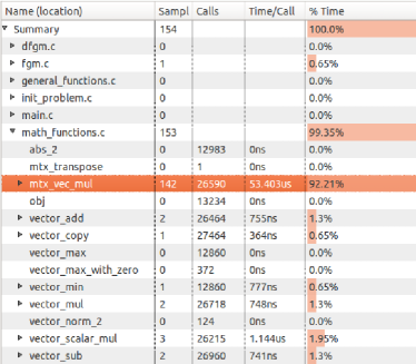
Figure 2: Profiling the code with gprof.

In conclusion, in DuQuad the main operations are the matrix-vector products. Therefore, DuQuad is adequate for solving QP problems on hardware with limited resources and capabilities, since it does not require any solver for linear systems or other complicating operations, while most of the existing solvers for QPs from the literature implementing e.g. active set or interior point methods require the capability of solving linear systems. On the other hand, DuQuad can be also used for solving large-scale sparse QP problems since the iterations are very cheap in this case (only sparse matrix-vector products).

6 Numerical simulations

DuQuad is mainly intended for small to medium size, dense QP problems, but it is of course also possible to use DuQuad to solve (sparse) QP instances of large dimension.

6.1 Distribution of DuQuad

The DuQuad software package is available for download from:

http://acse.pub.ro/person/ion-necoara

and distributed under general public license to allow linking against proprietary codes. Proceed to the menu point “Software” to obtain a zipped archive of the most current version of DuQuad. The user’s manual and extensive source code documentation are available here as well.

An overview of the workflow in DuQuad is illustrated in Fig. 3. A QP problem is constructed using a Matlab script called test.m. Then, the function duquad.m is called with the problem as input and is regarded as a prepossessing stage for the online optimization. The binary MEX file is called, with the original problem and the extra info as input. The main.c file of the C-code includes the MEX framework and is able to convert the MATLAB data into C format. Furthermore, the converted data gets bundled into a C struct and passed as input to the algorithm that solves the problem.

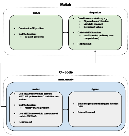
Figure 3: DuQuad workflow.

6.2 Numerical tests: case $\mathcal{K}=\{0\}$

We plot in Fig. 4 the average CPU time for several solvers, obtained by solving $50$ random QP’s with equality constraints ($Q\succeq 0$ and $\mathcal{K}=\{0\}$) for each dimension $n$, with an accuracy $\epsilon=0.01$ and the stopping criteria $\lvert F(\hat{u}^{k}_{\epsilon})-F^{*}\rvert$ and $\lVert G\hat{u}^{k}_{\epsilon}+g\rVert$ less than the accuracy $\epsilon$. In both algorithms DGM and DFGM we consider the average of iterates $\hat{u}^{k}_{\epsilon}$. Since $Q\succeq 0$, we have chosen $\rho={\cal O}(1/\epsilon)$. In the case of Algorithm DGM, at each outer iteration the inner problem is solved with accuracy $\epsilon_{\text{in}}=\epsilon$. For the Algorithm DFGM we consider two scenarios: in the first one, the inner problem is solved with accuracy $\epsilon_{\text{in}}=0.001$, while in the second one we use the theoretic inner accuracy (18). We observe a good behavior of Algorithm DFGM, comparable to Cplex and Gurobi.

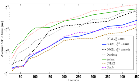
Figure 4: Average CPU time (ms) for solving QPs, with $Q\succeq 0$ and $\mathcal{K}=\{0\}$ of different dimensions, with several solvers.

6.3 Numerical tests: case $\mathcal{K}=\mathbb{R}^{p}_{-}$

We plot in Fig. 5 the number of iterations of Algorithms DGM and DFGM in the primal last and average iterates for $25$ random QPs with inequality constraints ($Q\succ 0$ and $\mathcal{K}=\mathbb{R}^{p}_{-}$) of variable dimension ranging from $n=10$ to $n=500$. We choose the accuracy $\epsilon=0.01$ and the stopping criteria was $\lvert F(u)-F^{*}\rvert$ and $\text{dist}_{\mathcal{K}}(Gu+g)$ less than the accuracy $\epsilon$. From this figure we observe that the number of iterations are not varying much for different test cases and also that the number of iterations are mildly dependent on problem’s dimension. Finally, we observe that dual first order methods perform usually better in the primal last iterate than in the average of primal iterates.

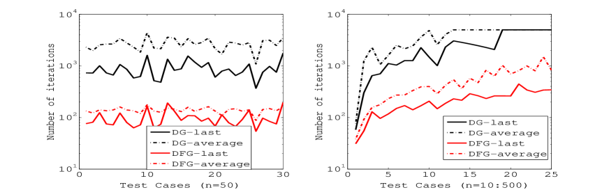
Figure 5: Number of outer iterations on random QPs ($Q\succ 0$, $\mathcal{K}=\mathbb{R}^{p}_{-}$) for DGM and DFGM in primal last/average of iterates for different test cases of the same dimension (left) and of variable dimension (right).

References

- (1) R. Bartlett and L. Biegler, QPSchur: a dual, active set, Schur complement method for large-scale and structured convex quadratic programming algorithm, Optimization and Engineering, 7:5-32, 2006.
- (2) A. Beck and M. Teboulle, A fast iterative shrinkage-thresholding algorithm for linear inverse problems, SIAM Journal on Imaging Sciences, 2(1):183–202, 2009.
- (3) A. Conn, N. Gould and Ph. Toint, LANCELOT: a Fortran package for large-scale nonlinear optimization, Springer Series in Computational Mathematics, Springer, 17, 1992.
- (4) O. Devolder, F. Glineur, Y. Nesterov, First-order methods of smooth convex optimization with inexact oracle Mathematical Programming 146 (1-2):37–75, 2014.
- (5) A. Domahidi, A. Zgraggen, M. Zeilinger, M. Morari and C. Jones, Efficient interior point methods for multistage problems arising in receding horizon control, IEEE Conference Decision and Control, 668–674, 2012.
- (6) M. Frank and P. Wolfe, An algorithm for quadratic programming, Naval Research Logistics Quarterly, 3(1-2):95–110, 1956.
- (7) P. Giselsson, Improved fast dual gradient methods for embedded model predictive control, Tech. rep., 2014.
- (8) J. Gondzio and A. Grothey, Parallel interior point solver for structured quadratic programs: application to financial planning problems, Annals of Operations Research, 152(1):319–339, 2007.
- (9) H. Ferreau, C. Kirches, A. Potschka, H. Bock and M. Diehl, qpOASES: a parametric active-set algorithm for quadratic programming, Mathematical Programming Computation, 2014.
- (10) J. Frasch, M. Vukov, H. Ferreau and M. Diehl, A new quadratic programming strategy for efficient sparsity exploitation in SQP-based nonlinear MPC and MHE, IFAC World Congress, 2014.
- (11) J. Jerez, K. Ling, G. Constantinides and E. Kerrigan, Model predictive control for deeply pipelined field-programmable gate array implementation: algorithms and circuitry, IET Control Theory and Applications, 6(8):1029–1041, 2012.
- (12) M. Kvasnica, P. Grieder, M. Baoti and M. Morari, Multi parametric toolbox (MPT), in Hybrid Systems: Computation and Control (R. Alur et al. Eds.), Springer, 2993:448–462, 2004.
- (13) G. Lan and R.D.C. Monteiro, Iteration-complexity of first-order augmented lagrangian methods for convex programming, Mathematical Programming, 2015.
- (14) J. Mattingley and S. Boyd, Automatic code generation for real-time convex optimization, in Convex Optimization in Signal Processing and Communications, Cambridge University Press, 2009.
- (15) I. Necoara and V. Nedelcu, Rate analysis of inexact dual first order methods: application to dual decomposition, IEEE Transactions on Automatic Control, 59(5):1232–1243, 2014.
- (16) V. Nedelcu, I. Necoara and Q. Tran Dinh, Computational complexity of inexact gradient augmented lagrangian methods: application to constrained MPC, SIAM Journal Control and Optimization, 52(5):3109–3134, 2014.
- (17) I. Necoara and V. Nedelcu, On linear convergence of a distributed dual gradient algorithm for linearly constrained separable convex problems, Automatica, 55(5):209-â216, 2015.
- (18) I. Necoara, L. Ferranti and T. Keviczky, An adaptive constraint tightening approach to linear MPC based on approximation algorithms for optimization, Optimal Control Applications and Methods, DOI: 10.1002/oca.2121, 1-19, 2015.
- (19) I. Necoara and A. Patrascu, Iteration complexity analysis of dual first order methods for conic convex programming, Tech. rep., Univ. Politehnica Bucharest, 1-35, 2014 (www.arxiv.org).
- (20) A. Nedic and A. Ozdaglar, Approximate primal solutions and rate analysis for dual subgradient methods, SIAM Journal on Optimization, 19(4):1757–1780, 2009.
- (21) Y. Nesterov, Introductory Lectures on Convex Optimization: A Basic Course, Kluwer, Boston, 2004.
- (22) Y. Nesterov, Gradient methods for minimizing composite functions, Mathematical Programming, 140(1):125–161, 2013.
- (23) P. Patrinos and A. Bemporad, An accelerated dual gradient-projection algorithm for embedded linear model predictive control, IEEE Transactions on Automatic Control, 59(1):18–33, 2014.
- (24) S. Richter, M. Morari and C. N. Jones, Towards computational complexity certification for constrained MPC based on lagrange relaxation and the fast gradient method, IEEE Conference Decision and Control, 5223–5229, 2011.
- (25) R.T. Rockafellar, Augmented Lagrangian and applications of the proximal point algorithm in convex programming, Mathematics Operation Research, 1:97-â116, 1976.
- (26) G. Stathopoulos, A. Szucs, Y. Pu and C. Jones, Splitting methods in control, European Control Conference, 2014.
- (27) P. Tseng, On accelerated proximal gradient methods for convex-concave optimization, SIAM Journal of Optimization, submitted:1–20, 2008.
- (28) F. Ullmann, FiOrdOs: a matlab toolbox for c-code generation for first order methods, Master thesis, ETH Zurich, 2011.
- (29) P.W. Wang and C.J. Lin, Iteration complexity of feasible descent methods for convex optimization, Journal of Machine Learning Research, 15:1523–1548, 2014.
- (30) E. Wei, A. Ozdaglar, and A. Jadbabaie, A distributed Newton method for network utility maximization–Part I and II, IEEE Transactions on Automatic Control, 58(9), 2013.
- (31) R.D. Zimmerman, C.E. Murillo-Sanchez and R.J. Thomas, Matpower: steady-state operations, planning, and analysis tools for power systems research and education, IEEE Transactions on Power Systems, 26(1):12–19, 2011.