Topologically driven nonequilibrium phase transitions in diagonal ensembles

Abstract

We identify a new class of topologically driven phase transitions when calculating the Hall conductance of two-band Chern insulators in the long-time limit after a global quench of the Hamiltonian. The Hall conductance is expressed as the integral of the Berry curvature in the diagonal ensemble. Even if the topological invariant of the wave function is conserved under unitary evolution, the Hall conductance as a function of the energy gap in the post-quench Hamiltonian displays a continuous but nonanalytic behavior, that is it has a logarithmically divergent derivative as the gap closes. The coefficient of this logarithmic function is the ratio of the change of Chern number in the ground state of the post-quench Hamiltonian to the energy gap in the initial state. This nonanalytic behavior is universal in two-band Chern insulators.

Introduction.– The discovery of the quantum Hall effect klitzing ; tsui , i.e. a quantized Hall conductance in the ground state which jumps from one plateau to another, inspired the study of topological order TKNN ; wen to characterize different topological phases outside the conventional framework of spontaneous symmetry breaking. Considerable effort has been devoted to understanding topological order or symmetry protected topological (SPT) order in the ground state. More recently, a lot of attention was devoted to the nature of topological order and SPT order for a state driven out of equilibrium, in particular for quantum quenches of the Hamiltonian tsomokos09 ; halasz13 ; rahmani10 ; foster ; fosterprb ; dong14 ; wang14 ; perfetto13 ; chung14 .

Consider an isolated system initially in the ground state of a Hamiltonian $\hat{H}_{i}$ and suddenly changing the Hamiltonian to $\hat{H}_{f}$. The wave function follows a unitary time evolution, while the local observables in the long time limit settle to the prediction of the diagonal ensemble rigol08 , which in some cases can be reduced to a thermal ensemble or a generalized Gibbs ensemble rigol07 ; polkovnikov . Topological order or SPT order cannot be expressed as a local observable. Therefore, its identification in a nonequilibrium state is far from trivial. In the toric code model, the topological entropy in the long time limit is found to be the same as its initial value independent from whether the ground states of $\hat{H}_{i}$ or $\hat{H}_{f}$ are topologically trivial or not tsomokos09 ; halasz13 ; rahmani10 . This result agrees with a universal argument for gapped spin liquids chen10 . Similarly, for the Fermi gas on a honeycomb lattice which essentially simulates the Haldane model, the Chern number is proved to be conserved under unitary evolution alessiol ; caio15 . However, in the two-dimensional topological superfluid, the winding number of the retarded Green’s function after a quench shows a strong dependence on the post-quench Hamiltonian $\hat{H}_{f}$ foster ; dong14 , even if the winding of the Anderson pseudo spin texture is conserved fosterprb . Also in the one-dimensional case, an analysis of tunneling spectroscopy by coupling the system to an auxiliary thermal bath shows that the SPT order is mostly determined by $\hat{H}_{f}$ wang14 . But in topological superconductors with proximity-induced superconductivity, the Majorana order parameter perfetto13 or the entanglement spectrum chung14 indicate that the quenched state is topologically trivial if $\hat{H}_{i}$ and $\hat{H}_{f}$ are in different topological phases.

To clarify the issue of SPT order far from equilibrium, we appeal to a measurable physical quantity, namely the Hall conductance in Chern insulators. We first study a paradigmatic model, i.e. the Dirac model shen , and then extend our results to a general two-band Chern insulator. We find that the Chern number of the unitarily evolving wave function is conserved and uniquely determined by $\hat{H}_{i}$. However, while the Hall conductance of the quenched state is a continuous function of the energy gap in $\hat{H}_{f}$, the derivative of this function displays a logarithmic divergence whenever the Chern number of the ground state of $\hat{H}_{f}$ changes. We thus identify a new class of topologically driven phase transitions with an exotic critical behavior, which is quite different from the orthodox one in which the Hall conductance is discontinuous but its derivative is zero everywhere in the phase diagram. The discrepancy in the SPT order obtained from the Chern number (based on unitary time evolution) and the Hall conductance is attributed to the fact that the latter must be calculated from the diagonal ensemble, in which the coherence between different eigenstates of $\hat{H}_{f}$ in the wave function is lost in the long-time limit. In this experimentally relevant sense the SPT order of quenched states depends on $\hat{H}_{f}$.

Real-time dynamics of the Chern number.– The Hamiltonian of a two-band Chern insulator in two dimensions is expressed as

$$\hat{H}=\sum_{\vec{k}}\hat{c}^{\dagger}_{\vec{k}}\mathcal{H}_{\vec{k}}\hat{c}_{\vec{k}},$$ (1)

where $\hat{c}_{\vec{k}}=\left(\hat{c}_{\vec{k}1},\hat{c}_{\vec{k}2}\right)^{T}$ is the fermionic operator and $\sum_{\vec{k}}$ sums over a single Brillouin zone. The single-particle Hamiltonian $\mathcal{H}_{\vec{k}}$ can be decomposed into $\mathcal{H}_{\vec{k}}=\vec{d}_{\vec{k}}\cdot\vec{\sigma}$, where $\vec{\sigma}$ denotes the Pauli matrices.

The Dirac model is a paradigm for two-band Chern insulators shen . In the Dirac model, the coefficients of the Pauli matrices are $\vec{d}_{\vec{k}}=(k_{x},k_{y},M-Bk^{2})$ with two parameters $M$ and $B$, and $\sum_{\vec{k}}$ sums over the whole momentum plane. The ground state is well known to be classified by the Chern number $C=\frac{1}{2}\left(\textbf{sgn}(M)+\textbf{sgn}(B)\right)$, which is quantized and changes only at the phase boundary $M=0$ or $B=0$. The Hall conductance of the ground state is simply the Chern number in units of $e^{2}/h$.

At the time $t=0$, we suddenly change the Hamiltonian from $\hat{H}_{i}=\hat{H}(M_{i},B_{i})$ to $\hat{H}_{f}=\hat{H}(M_{f},B_{f})$. Then the wave function evolves according to $|\Psi(t)\rangle=e^{-i\hat{H}_{f}t}|\Psi(0)\rangle=\prod_{\vec{k}}\otimes|u_{\vec{k}}(t)\rangle$, where $|u_{\vec{k}}(t)\rangle$ is the single-particle wave function obeying $\mathcal{H}_{\vec{k}}^{f}|u_{\vec{k}}(t)\rangle=i\frac{\partial}{\partial t}|u_{\vec{k}}(t)\rangle$. The momentum is a good quantum number both in $\hat{H}_{i}$ and $\hat{H}_{f}$. Therefore, it is natural to generalize the definition of the Chern number for the time-dependent wave function in the following way:

$$C(t)=\frac{i}{2\pi}\int d\vec{k}^{2}\left(\Braket{\frac{\partial u_{\vec{k}}(t)}{\partial k_{x}}}{\frac{\partial u_{\vec{k}}(t)}{\partial k_{y}}}-\text{H.c.}\right).$$ (2)

This real-time Chern number characterizes the topological property of the wave function $|\Psi(t)\rangle$, and can be reexpressed as $C(t)=\frac{i}{2\pi}\int d\vec{S}\cdot\left(\triangledown_{\vec{k}}\times\vec{A}(t)\right)$, where $\vec{S}$ denotes the $k_{x}$-$k_{y}$ plane oriented in the $k_{z}$-direction and $\vec{A}(t)=\langle u_{\vec{k}}(t)|\triangledown_{\vec{k}}|u_{\vec{k}}(t)\rangle$ is the Berry connection. $C(t)$ is determined by the poles of $\vec{A}(t)$ and must remain quantized at all times since locally deforming $\vec{A}(t)$ cannot change it. In fact, the two poles of $\vec{A}(t)$ at $k=0$ and $k=\infty$ have conserved residues under a unitary evolution supp , so that for arbitrary $\hat{H}_{i}$ and $\hat{H}_{f}$ we have $C(t)\equiv C(0)$. The Chern number of the wave function never changes although the system is driven out of equilibrium, which agrees with the no-go theorem proved by D’Alessio and Rigol alessiol . This result suggests that the SPT order of a wave function is generally conserved after a quench if the Hamiltonian in real space contains only local operators chen10 .

Hall conductance in the diagonal ensemble.– The observation that $C(t)$ is independent of $\hat{H}_{f}$ does not imply the absence of nonequilibrium phase transitions because $C(t)$ is not a measurable physical quantity. In this paper, a nonequilibrium phase transition is unambiguously indicated by the nonanalytic behavior of observables as the post-quench Hamiltonian $\hat{H}_{f}$ changes. We choose the Hall conductance as the indicator of nonequilibrium phase transitions. Notice that in the ground state the Hall conductance is directly related to the Chern number.

It is well known that the Hall conductance cannot be expressed as the expectation value of a local operator, but must be written as the long-time response to an external electric field in linear response theory. This fact reflects the topological nature of the Hall conductance and is related to the observation that in order to measure the Hall conductance, one must couple the system to auxiliary reservoirs. However, coupling to reservoirs unavoidably introduces decoherence and therefore in the long-time limit the far-from-equilibrium system will be described by the diagonal ensemble and not the unitarily evolved wave function of the isolated system. This motivates us to pursue a definition of SPT order and topologically driven nonequilibrium phase transitions by studying the Hall conductance in the diagonal ensemble, which is the experimentally relevant setting. In the long-time limit, the off-diagonal terms of the density matrix in the eigenbasis of $\hat{H}_{f}$ are averaged out rigol08 . The time-averaged expectation value of an operator $\hat{O}$ can be expressed as

$$\begin{split}\lim_{T\to\infty}\frac{1}{T}\int^{T}_{0}dt\langle\Psi(t)|\hat{O}|\Psi(t)\rangle&=\sum_{E}|\langle E|\Psi(0)\rangle|^{2}\langle E|\hat{O}|E\rangle\\ &=\textbf{Tr}[\hat{O}\hat{\rho}],\end{split}$$ (3)

where $|E\rangle$ are the eigenstates of $\hat{H}_{f}$ and $\hat{\rho}$ is diagonal in the basis $|E\rangle$ with the elements $|\langle E|\Psi(0)\rangle|^{2}$. If the long-time limit of $\langle\Psi(t)|\hat{O}|\Psi(t)\rangle$ exists, it must be determined by $\hat{\rho}$, the so-called diagonal ensemble rigol08 . While this argument is based on non-degenerate eigenenergies, the applicability of the diagonal ensemble has also been shown in many integrable quantum many-body models rigol09 ; ziraldo .

We build our formalism on the diagonal ensemble with the density matrix written as

$$\hat{\rho}=\prod_{\vec{k}}\otimes\left(\sum_{\alpha=\pm}n_{\vec{k}\alpha}|u^{f}_{\vec{k}\alpha}\rangle\langle u^{f}_{\vec{k}\alpha}|\right),$$ (4)

where $|u^{f}_{\vec{k}\alpha}\rangle$ is the eigenvector of $\mathcal{H}_{\vec{k}}^{f}$ and $\alpha=\pm$ denotes the upper and lower bands with the positive and negative eigenvalues $\pm|\vec{d}^{f}_{\vec{k}}|$, respectively. $n_{\vec{k}\alpha}$ is the occupation number of the band $\alpha$ and can be expressed as the overlap $n_{\vec{k}\alpha}=|\langle u^{f}_{\vec{k}\alpha}|u^{i}_{\vec{k}-}\rangle|^{2}$, where $|u^{i}_{\vec{k}-}\rangle$ is the lower-band eigenvector of the initial Hamiltonian $\mathcal{H}_{\vec{k}}^{i}$, which is in fact the initial wave function. The total occupation at each $\vec{k}$ is conserved to be $n_{\vec{k}+}+n_{\vec{k}-}\equiv 1$. Eq. (4) is obtained by averaging out the off-diagonal elements in $\left(|u_{\vec{k}}(t)\rangle\langle u_{\vec{k}}(t)|\right)$.

Now we calculate the Hall conductance of the diagonal ensemble in linear response theory mahan , i.e., we replace the equilibrium density matrix in linear response theory by the diagonal ensemble $\hat{\rho}$. This replacement does not cause any problem in the formalism because $\hat{\rho}$ is time-independent satisfying $[\hat{\rho},\hat{H}_{f}]=0$. We can then express the Hall conductance as the current-current correlation in the diagonal ensemble:

$$\sigma_{H}=\lim_{\omega\to 0}\frac{1}{S\omega}\int^{\infty}_{0}dte^{i\omega t}\textbf{Tr}\left(\hat{\rho}\left[\hat{J}_{y},\hat{J}_{x}(t)\right]\right),$$ (5)

where $S$ denotes the area of the system and is conventionally set to unity. $\hat{J}_{\beta}=e\sum_{\vec{k}}\hat{c}^{\dagger}_{\vec{k}}\displaystyle\frac{\partial\mathcal{H}^{f}_{\vec{k}}}{\partial k_{\beta}}\hat{c}_{\vec{k}}$ is the current operator along the $\beta$-direction with $e$ denoting the charge of the particle. Following the process for obtaining the celebrated TKNN number TKNN , we reexpress the dimensionless Hall conductance $C_{neq}:=\sigma_{H}/(e^{2}/h)$ as supp

$$C_{neq}=\frac{i}{2\pi}\sum_{\alpha}\int d\vec{k}^{2}n_{\vec{k}\alpha}\left(\Braket{\frac{\partial u^{f}_{\vec{k}\alpha}}{\partial k_{x}}}{\frac{\partial u^{f}_{\vec{k}\alpha}}{\partial k_{y}}}-\text{H.c.}\right),$$ (6)

which is the integral of the weighted mixture of Berry curvatures in different bands of the post-quench Hamiltonian. In the case of $\hat{H}_{i}=\hat{H}_{f}$ (no quench), the occupation is $n_{\vec{k}-}=1$ and $n_{{\vec{k}+}}=0$ everywhere in the Brillouin zone, and $C_{neq}$ is just the Chern number of the initial state as we expect. But for $\hat{H}_{i}\neq\hat{H}_{f}$, $n_{\vec{k}\alpha}\in[0,1]$ becomes a continuous function of $\vec{k}$ so that $C_{neq}$ is not quantized any more but can take an arbitrary value.

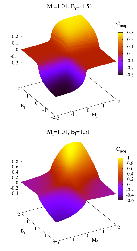
Figure 1: (Color online) The Hall conductance $C_{neq}$ as a function of $(M_{f},B_{f})$ at different $(M_{i},B_{i})$ in the Dirac model. [Top panel] The initial state is topologically trivial. [Bottom panel] The initial state is topologically nontrivial.

It is worth comparing the real time Chern number $C(t)$ in Eq. (2) with the dimensionless Hall conductance $C_{neq}$ in Eq. (6). The former reflects the topology of the wave function, being quantized but not measurable, while the latter is a true observable but not quantized. They are both integrals of the Berry curvature, but $C(t)$ is derived from the wave function while $C_{neq}$ follows from the diagonal ensemble where the coherence is lost. Decoherence plays a crucial role in understanding the SPT order of a quenched state in the long-time limit which is a nonequilibrium steady state.

Nonanalytic behavior of Hall conductance.– In the Dirac model, it is straightforward to determine the Hall conductance as supp

$$C_{neq}=\int_{0}^{\infty}d\tilde{k}\frac{\left(\tilde{k}+(B_{i}\tilde{k}-M_{i})(B_{f}\tilde{k}-M_{f})\right)\left(B_{f}\tilde{k}+M_{f}\right)}{4d^{i}_{\vec{k}}\left(d^{f}_{\vec{k}}\right)^{4}}$$ (7)

with $d^{i/f}_{\vec{k}}=\sqrt{\tilde{k}+(B_{i/f}\tilde{k}-M_{i/f})^{2}}$. The Hall conductance $C_{neq}$ is a function of $(M_{i},B_{i},M_{f},B_{f})$, i.e., the parameters of $\hat{H}_{i}$ and $\hat{H}_{f}$. This function satisfies the properties:

$$\begin{split}C_{neq}(M_{i},B_{i},M_{f},B_{f})=&C_{neq}(B_{i},M_{i},B_{f},M_{f})\\ =&-C_{neq}(-M_{i},-B_{i},-M_{f},-B_{f}).\end{split}$$ (8)

Let us study this function as $(M_{f},B_{f})$ changes, while $(M_{i},B_{i})$ is invariant, i.e., the initial state is fixed. Due to Eq. (8), we only consider the cases $M_{i},B_{i}>0$ and $M_{i}>0,B_{i}<0$. As shown in Fig. 1, $C_{neq}$ is a continuous function of $(M_{f},B_{f})$ in the whole parameter space supp . This result is surprising if we consider the fact that the Chern number of the ground state has a jump whenever $M$ or $B$ change sign. By driving the system out of equilibrium, we smoothen the Hall conductance function. $C_{neq}(M_{f},B_{f})$ has a similar shape at different $(M_{i},B_{i})$, reminiscent of the function $(\textbf{sgn}(M_{f})+\textbf{sgn}(B_{f}))/2$, i.e., the Chern number in the ground-state wave function of the post-quench Hamiltonian $\hat{H}_{f}$. As $M_{f},B_{f}\gg 0$ ($M_{f},B_{f}\ll 0$), $C_{neq}$ takes a positive (negative) value, while $C_{neq}$ is close to zero as $M_{f}$ and $B_{f}$ have different signs. Even if the initial state is topologically trivial (see Fig. 1, the top panel), the Hall conductance is finite as $\hat{H}_{f}$ is in the nontrivial regime, but it cannot reach the quantized values $\pm e^{2}/h$. When the initial state is nontrivial (see Fig. 1, the bottom panel), the Hall conductance is suppressed as $\hat{H}_{f}$ deviates from $\hat{H}_{i}$, and can even change the sign as $M_{f}$ and $B_{f}$ both change their signs.

While $C_{neq}(M_{f},B_{f})$ is continuous, the key finding is that whenever the post-quench Hamiltonian crosses the boundary at $M_{f}=0$ ($B_{f}=0$), the derivative of the Hall conductance $\frac{\partial C_{neq}}{\partial M_{f}}$ ($\frac{\partial C_{neq}}{\partial B_{f}}$) diverges to $+\infty$ in a logarithmic way supp :

$$\begin{split}&\lim_{M_{f}\to 0}\frac{\partial C_{neq}}{\partial M_{f}}\sim\frac{-1}{2|M_{i}|}\ln|M_{f}|,\\ &\lim_{B_{f}\to 0}\frac{\partial C_{neq}}{\partial B_{f}}\sim\frac{-1}{2|B_{i}|}\ln|B_{f}|.\end{split}$$ (9)

As $M_{f}\to 0$, $\frac{\partial C_{neq}}{\partial M_{f}}$ as a function of $\left(\ln|M_{f}|\right)$ asymptotically approaches a straight line with the slope $-1/(2|M_{i}|)$, which is independent of $B_{f},B_{i}$ and the side from which $M_{f}$ goes to zero. As $B_{f}\to 0$, $\frac{\partial C_{neq}}{\partial B_{f}}$ has a similar divergence since $C_{neq}$ is invariant under the exchange of $M_{f}$ and $B_{f}$ according to Eq. (8). We identify a nonequilibrium phase transition when the Chern number in the ground state of $\hat{H}_{f}$ changes. The critical behavior of this phase transition is exotic, compared to that of ground-state phase transitions in which the Hall conductance has a zero derivative everywhere but displays a discontinuity at the phase boundary.

This phase transition reveals different nonequilibrium phases which share the common symmetries of the Dirac model. Apparently, the broken symmetry picture does not account for this transition, which must be topologically driven. Interestingly, the topological invariant of the wave function $C(t)$ is independent of $(M_{f},B_{f})$, and then fails to characterize different phases in this nonequilibrium phase transition. One can assign the Chern number $C(\hat{H}_{f})$ of the ground-state wave function of $\hat{H}_{f}$ to each nonequilibrium phase to distinguish them. We will see that the change of $C(\hat{H}_{f})$ determines the character of this nonequilibrium phase transition in a general two-band Chern insulator.

Now let us consider a general two-band Chern insulator in two dimensions with the Hamiltonian given by Eq. (1). The coefficient vector $\vec{d}_{\vec{k}}=\left(d_{1\vec{k}},d_{2\vec{k}},d_{3\vec{k}}\right)$ is different from model to model. But the nonanalytic behavior of Hall conductance is insensitive to the change of $\vec{d}_{\vec{k}}$. Instead, it depends only upon the lowest-order expansion of $\vec{d}_{\vec{k}}$ at the momentum $\vec{q}$ where the energy gap closes ($d_{\vec{q}}=0$) at a phase boundary. In a generic model, two components of $\vec{d}_{\vec{q}}$ must be zero. Let us suppose them to be $d_{1\vec{q}}$ and $d_{2\vec{q}}$ without loss of generality. The energy gap is $d_{\vec{q}}=|d_{3\vec{q}}|$ when the system is close to the phase boundary. $d_{3\vec{q}}$ is a free parameter in the Hamiltonian (the gap parameter), which is denoted by $m$. Note that $m=M$ in the Dirac model.

Suppose that the system is initially in a ground state with the gap parameter $m=m_{i}$, before we suddenly change $m$ in the Hamiltonian from $m_{i}$ to $m_{f}$. We measure the Hall conductance in the long time limit. The Hall conductance $C_{neq}$ is a function of $m_{f}$, while we fix $m_{i}$ to be nonzero. The function $C_{neq}(m_{f})$ is continuous but nonanalytic at $m_{f}=0$, where the gap of the post-quench Hamiltonian $\hat{H}_{f}$ closes. The derivative of $C_{neq}(m_{f})$ satisfies supp

$$\lim_{m_{f}\to 0}\frac{dC_{neq}}{dm_{f}}\sim\frac{\displaystyle\lim_{m_{f}\to 0^{-}}C(m_{f})-\displaystyle\lim_{m_{f}\to 0^{+}}C(m_{f})}{2|m_{i}|}\ln|m_{f}|,$$ (10)

where $C(m_{f})$ denotes the Chern number in the ground-state wave function of $\hat{H}_{f}$. The derivative of the Hall conductance with respect to the energy gap in $\hat{H}_{f}$ is logarithmically divergent as the gap closes. And the coefficient of this logarithmic function is the ratio of the change of Chern number in the ground state of $\hat{H}_{f}$ to the energy gap in the initial state. Eq. (10) relates the nonequilibrium phase transition in quenched states to the topological phase transition in ground states, indicating that this nonequilibrium phase transition is in fact topologically driven. Eq. (9) for the Dirac model is a special case of Eq. (10) as the change of Chern number is $-1$.

Conclusions.– In summary, we find a new class of topologically driven phase transitions in quenched states of two-band Chern insulators, which are characterized by the Hall conductance as a continuous function of the energy gap in the post-quench Hamiltonian $\hat{H}_{f}$ with a logarithmically divergent derivative. The asymptotic behavior of the Hall conductance function is determined by the ratio of the change of Chern number in the ground state of $\hat{H}_{f}$ to the energy gap in the initial state, which is universal in two-band Chern insulators. We obtain the Hall conductance by applying linear response theory in the diagonal ensemble of the system, which is the physically correct description of the long-time limit in a far-from-equilibrium quench setup. The topological invariant of the real-time wave function fails to predict this phase transition, which can only be correctly identified in the diagonal ensemble where decoherence effects are taken into account. Our finding indicates the possibility of exotic topological phase transitions in systems far from equilibrium.

Finally, we discuss the conditions for observing this phase transition in experiments. The nonequilibrium distribution of particles is responsible for the logarithmically divergent derivative of the Hall conductance. Ultracold atomic gases are known to be well isolated from the environment and suitable for studying the quench dynamics of many-body quantum systems greiner . The Haldane model haldane was recently realized with cold atoms in an optical lattice jotzu14 . The Haldane model is a two-band Chern insulator, in which the quenched-state Hall conductance displays the nonanalytic behavior in Eq. (10) universalargue . The measurement of conductances in cold atoms is difficult, but a two-terminal setup was implemented recently brantut12 ; stadler12 . We expect that our prediction can be checked in a four-terminal setup made of cold atoms simulating the Haldane model.

Acknowledgement.– We thank Prof. Q. Niu for inspiring discussions. We thank J. Oberreuter and M. Medvedyeva for their help in preparing the paper. Pei Wang is supported by NSFC under Grant No. 11304280, and by China Scholarship Council. S. K. was supported through SFB 1073 (project B03) of the Deutsche Forschungsgemeinschaft (DFG).

Supplementary material

Appendix A The real-time Chern number $C(t)$ in the Dirac model

We express the real-time Chern number as

$$C(t)=\frac{i}{2\pi}\int d\vec{S}\cdot\left(\triangledown_{\vec{k}}\times\vec{A}(t)\right),$$ (11)

where $\vec{A}(t)=\langle u_{\vec{k}}(t)|\triangledown_{\vec{k}}|u_{\vec{k}}(t)\rangle$ is the Berry connection with $|u_{\vec{k}}(t)\rangle=(\phi_{1},\phi_{2})^{T}$ denoting the single-particle wave function. In the Dirac model, it is straightforward to calculate the wave function and obtain

$$\begin{split}\phi_{1}(t)=&\frac{1}{\sqrt{2d^{i}_{\vec{k}}(d^{i}_{\vec{k}}-d^{i}_{3\vec{k}})}}\big{[}-\cos(d^{f}_{\vec{k}}t)(d^{i}_{\vec{k}}-d^{i}_{3\vec{k}})\\ &+i\sin(d^{f}_{\vec{k}}t)\frac{d^{f}_{3\vec{k}}\left(d^{i}_{\vec{k}}-d^{i}_{3\vec{k}}\right)-k^{2}}{d^{f}_{\vec{k}}}\big{]},\end{split}$$ (12)

and

$$\begin{split}\phi_{2}(t)=&\frac{k_{+}}{2d^{f}_{\vec{k}}\sqrt{2d^{i}_{\vec{k}}(d^{i}_{\vec{k}}-d^{i}_{3\vec{k}})}}\big{[}2d^{f}_{\vec{k}}\cos(d^{f}_{\vec{k}}t)\\ &+2i\sin(d^{f}_{\vec{k}}t)(d^{i}_{\vec{k}}-d^{i}_{3\vec{k}}+d^{f}_{3\vec{k}})\big{]},\end{split}$$ (13)

where $k_{+}=k_{x}+ik_{y}$, $\vec{d}^{i/f}_{\vec{k}}=(d^{i/f}_{1\vec{k}},d^{i/f}_{2\vec{k}},d^{i/f}_{3\vec{k}})$ is the coefficient vector in the initial and post-quench Hamiltonians, respectively, and ${d}^{i/f}_{\vec{k}}$ is the length of $\vec{d}^{i/f}_{\vec{k}}$. We divide the Berry connection into $\vec{A}(t)=\vec{A}_{1}(t)+\vec{A}_{2}(t)$ with $\vec{A}_{\alpha}=\phi^{*}_{\alpha}\triangledown_{\vec{k}}\phi_{\alpha}$. Noticing that $\phi_{1}$ is a function of $k=\sqrt{k_{x}^{2}+k_{y}^{2}}$, we immediately know that $\left(\triangledown_{\vec{k}}\times\vec{A}_{1}\right)$ must be zero, so that $\vec{A}_{1}$ does not contribute to $C(t)$. We again divide $\vec{A}_{2}$ into the irrelevant term $\vec{A}_{2a}$ with a zero curl and the relevant term $\vec{A}_{2b}$ with its imaginary part written as

$$\begin{split}\textbf{Im}[\vec{A}_{2b}]=&\left[\cos^{2}(d^{f}_{\vec{k}}t)+\sin^{2}(d^{f}_{\vec{k}}t)\frac{(d^{i}_{\vec{k}}-d^{i}_{3\vec{k}}+d^{f}_{3\vec{k}})^{2}}{\left(d^{f}_{\vec{k}}\right)^{2}}\right]\\ &\times\frac{-k_{y}\vec{x}+k_{x}\vec{y}}{2d^{i}_{\vec{k}}(d^{i}_{\vec{k}}-d^{i}_{3\vec{k}})},\end{split}$$ (14)

where $\vec{x}$ and $\vec{y}$ denote the unit vectors in the momentum plane.

Now we reexpress the Chern number by the vector field $\textbf{Im}[\vec{A}_{2b}]$ as

$$C(t)=\frac{-1}{2\pi}\int d\vec{S}\cdot\left(\triangledown_{\vec{k}}\times\textbf{Im}[\vec{A}_{2b}(t)]\right).$$ (15)

$\textbf{Im}[\vec{A}_{2b}]$ is a vortex field with two poles at zero and infinity, respectively. Applying the Kelvin-Stokes theorem in an annulus with inner radius $r$ and outer radius $R$, and then taking the limit $r\to 0$ and $R\to\infty$, we obtain

$$\begin{split}-2\pi C(t)=&\lim_{r\to 0,R\to\infty}\int_{r\leq k\leq R}d\vec{S}\cdot\left(\triangledown_{\vec{k}}\times\textbf{Im}[\vec{A}_{2b}]\right)\\ =&\left(\lim_{R\to\infty}\oint_{k=R}-\lim_{r\to 0}\oint_{k=r}\right)\textbf{Im}[\vec{A}_{2b}]\cdot d\vec{k}\\ =&\lim_{R\to\infty}\left(2\pi R|\textbf{Im}[\vec{A}_{2b}]|_{k=R}\right)\\ &-\lim_{r\to 0}\left(2\pi r|\textbf{Im}[\vec{A}_{2b}]|_{k=r}\right),\end{split}$$ (16)

where $|\textbf{Im}[\vec{A}_{2b}]|_{k=R}$ denotes the length of the vector $\textbf{Im}[\vec{A}_{2b}]$ at the circle of radius $\left(k=R\right)$. The first limit evaluates $\big{(}\pi(1-\textbf{sgn}(B_{i}))\big{)}$, while the second limit evaluates $\big{(}\pi(1+\textbf{sgn}(M_{i}))\big{)}$, being both time-independent. In other words, the residues of $\textbf{Im}[\vec{A}_{2b}]$ at zero and infinity are both time-invariant, which leads to a conserved Chern number:

$$C(t)\equiv\frac{1}{2}\left(\textbf{sgn}(M_{i})+\textbf{sgn}(B_{i})\right).$$ (17)

Appendix B The Hall conductance of quenched states

In this section, we first show how to express the Hall conductance of quenched states as the integral of the Berry curvature. Our derivation is a straightforward extension of the work by Thouless et al. TKNN:app . We then express the Hall conductance by using the coefficient vectors in two-band Chern insulators.

In linear response theory, the Hall conductance is written as

$$\sigma_{H}=\lim_{\omega\to 0}\frac{1}{S\omega}\int^{\infty}_{0}dte^{i\omega t-\eta|t|}\textbf{Tr}\left(\hat{\rho}\left[\hat{J}_{y},\hat{J}_{x}(t)\right]\right),$$ (18)

where $\eta$ is an infinitesimal number corresponding to the adiabatic switch-on of an external electric field, and $\omega$ is the frequency of the electric field with the limit ${\omega\to 0}$ corresponding to the dc-conductance. The diagonal ensemble is known to be $\hat{\rho}=\prod_{\vec{k}}\otimes\left(\sum_{\alpha}n_{\vec{k}\alpha}|u^{f}_{\vec{k}\alpha}\rangle\langle u^{f}_{\vec{k}\alpha}|\right)$, which is a product state. Due to the conversation law $\sum_{\alpha}n_{\vec{k}\alpha}=1$, the state of the system is limited in a subspace of the Fock space in which the empty or doubly-occupied states at each momentum are excluded. We can then reexpress $\sigma_{H}$ in the first-quantization language as

$$\begin{split}\sigma_{H}=\lim_{\omega\to 0}\frac{1}{S\omega}\int^{\infty}_{0}&dte^{i\omega t-\eta|t|}\\ &\times\sum_{\vec{k},\alpha}n_{\vec{k}\alpha}\Bra{u^{f}_{\vec{k}\alpha}}\left[\hat{J}^{y}_{\vec{k}},\hat{J}^{x}_{\vec{k}}(t)\right]\Ket{u^{f}_{\vec{k}\alpha}},\end{split}$$ (19)

where the momentum-resolved current operator is $\hat{J}^{\beta}_{\vec{k}}=e\displaystyle\frac{\partial\mathcal{H}^{f}_{\vec{k}}}{\partial k_{\beta}}$. Since we are interested in the dc Hall conductance which is a real number, we take the real part of $\sigma_{H}$ and obtain

$$\begin{split}\textbf{Re}\sigma_{H}=&\frac{\sigma_{H}+\sigma_{H}^{*}}{2}\\ =&\frac{-ie^{2}}{S}\sum_{\vec{k},\alpha,\beta}\frac{n_{\vec{k}\alpha}}{(\epsilon_{\vec{k}\alpha}-\epsilon_{\vec{k}\beta})^{2}}\\ &\times\biggl{[}\Bra{u^{f}_{\vec{k}\alpha}}\frac{\partial\mathcal{H}^{f}_{\vec{k}}}{\partial k_{y}}\Ket{u^{f}_{\vec{k}\beta}}\Bra{u^{f}_{\vec{k}\beta}}\frac{\partial\mathcal{H}^{f}_{\vec{k}}}{\partial k_{x}}\Ket{u^{f}_{\vec{k}\alpha}}-\text{H.c.}\biggr{]},\end{split}$$ (20)

where $\epsilon_{\vec{k}\alpha}$ denotes the eigenvalue of $\mathcal{H}^{f}_{\vec{k}}$. We make use of the relation $\mathcal{H}^{f}_{\vec{k}}=\sum_{\alpha}\epsilon_{\vec{k}\alpha}|u^{f}_{\vec{k}\alpha}\rangle\langle u^{f}_{\vec{k}\alpha}|$ and finally obtain

$$\begin{split}C_{neq}=&\frac{\textbf{Re}\sigma_{H}}{e^{2}/h}\\ =&\frac{i}{2\pi}\sum_{\alpha}\int d\vec{k}^{2}n_{\vec{k}\alpha}\left(\Braket{\frac{\partial u^{f}_{\vec{k}\alpha}}{\partial k_{x}}}{\frac{\partial u^{f}_{\vec{k}\alpha}}{\partial k_{y}}}-\text{H.c.}\right).\end{split}$$ (21)

In a two-band Chern insulator with the Hamiltonian $\mathcal{H}_{\vec{k}}=\vec{d}_{\vec{k}}\cdot\vec{\sigma}$, the Berry curvatures in different bands are opposite to each other. By using this and the conservation law $n_{\vec{k}+}+n_{\vec{k}-}\equiv 1$, we reexpress Eq. (21) as

$$C_{neq}=\int d\vec{k}^{2}\cos\theta\cdot\mathcal{C},$$ (22)

where $\mathcal{C}$ denotes the Berry curvature in the lower-band of the post-quench Hamiltonian $\hat{H}_{f}$ and can be expressed as

$$\mathcal{C}=\frac{\left(\displaystyle\frac{\partial\vec{d}^{f}_{\vec{k}}}{\partial k_{x}}\times\frac{\partial\vec{d}^{f}_{\vec{k}}}{\partial k_{y}}\right)\cdot\vec{d}^{f}_{\vec{k}}}{4\pi(d^{f}_{\vec{k}})^{3}},$$ (23)

and $\cos\theta$ is the occupation factor defined as

$$\begin{split}\cos\theta:=&(2n_{\vec{k}-}-1)\\ =&(\vec{d}^{f}_{\vec{k}}\cdot\vec{d}^{i}_{\vec{k}})/({d}^{f}_{\vec{k}}{d}^{i}_{\vec{k}})\end{split}$$ (24)

with $\theta$ denoting the angle between $\vec{d}^{i}_{\vec{k}}$ and $\vec{d}^{f}_{\vec{k}}$. $\vec{d}^{i}_{\vec{k}}$ and $\vec{d}^{f}_{\vec{k}}$ are the coefficients of the Pauli matrices in the initial and post-quench Hamiltonians, respectively, and ${d}^{i}_{\vec{k}}$ and ${d}^{f}_{\vec{k}}$ are the length of $\vec{d}^{i}_{\vec{k}}$ and $\vec{d}^{f}_{\vec{k}}$, respectively.

Appendix C Continuity and nonanalyticity of the Hall conductance in the Dirac model

In this section, we show how to prove the continuity of $C_{neq}(M_{f},B_{f})$ and the logarithmic divergence of its derivative at the phase boundary. We only prove the case at $M_{f}=0$ when $B_{f}$ is fixed to be nonzero, since $C_{neq}(M_{f},B_{f})$ is invariant under the exchange of $M_{f}$ and $B_{f}$.

In the Dirac model, both $\mathcal{C}$ and $\cos\theta$ are rotationally invariant in the $k_{x}$-$k_{y}$ plane. We can then carry out the azimuthal integration in Eq. (22). By making a substitution $\tilde{k}=k^{2}$, we express the Hall conductance as

$$C_{neq}=\int_{0}^{\infty}d\tilde{k}\cos\theta\cdot\mathcal{C},$$ (25)

where the Berry curvature is

$$\mathcal{C}=\frac{1}{4}\frac{B_{f}\tilde{k}+M_{f}}{\left(d^{f}_{\vec{k}}\right)^{3}},$$ (26)

and the occupation factor is

$$\cos\theta=\frac{\tilde{k}+(B_{i}\tilde{k}-M_{i})(B_{f}\tilde{k}-M_{f})}{d^{i}_{\vec{k}}d^{f}_{\vec{k}}}$$ (27)

with $d^{i/f}_{\vec{k}}=\sqrt{\tilde{k}+(B_{i/f}\tilde{k}-M_{i/f})^{2}}$. At $M_{f}\neq 0$, we can express the derivative of $C_{neq}$ as

$$\frac{\partial{C_{neq}}}{\partial M_{f}}=\int_{0}^{\infty}d\tilde{k}\frac{\partial(\cos\theta\cdot\mathcal{C})}{\partial M_{f}}.$$ (28)

A straightforward observation is that both $\cos\theta(\tilde{k})$ and $\mathcal{C}(\tilde{k})$ are smooth functions for $\tilde{k}\in(0,\infty)$. However, they do not uniformly converge to $(\cos\theta)_{M_{f}=0}$ or $\mathcal{C}_{M_{f}=0}$ as $M_{f}\to 0$. The unique singularity is $\tilde{k}=0$, at which we have $\lim_{\tilde{k}\to 0}\lim_{M_{f}\to 0}\cos\theta=0$ but $\lim_{M_{f}\to 0}\lim_{\tilde{k}\to 0}\cos\theta=\textbf{sgn}(M_{i})\textbf{sgn}(M_{f})$. And $\mathcal{C}\left(\tilde{k}=0\right)=\textbf{sgn}(M_{f})/(4M_{f}^{2})$ is divergent as $M_{f}\to 0$. We divide the integral into two parts: $\int_{0}^{\infty}d\tilde{k}=\int_{0}^{\eta}d\tilde{k}+\int_{\eta}^{\infty}d\tilde{k}$ with $\eta>0$ a number that can be arbitrarily small. The second integral is a smooth function of $M_{f}$, which can be proved by studying the asymptotic behavior of $(\cos\theta\cdot\mathcal{C})$ in the limit $\tilde{k}\to\infty$, or more precisely, by making a substitution $\tilde{k}\to 1/\tilde{k}$ in the integral. In fact, $\tilde{k}=\infty$ is a true singularity at the boundary $B_{f}=0$, where $\tilde{k}=0$ is a regular point, since $\cos\theta$ and $\mathcal{C}$ are invariant under the substitution $\tilde{k}\leftrightarrow 1/\tilde{k}$ and $M_{i/f}\leftrightarrow B_{i/f}$. If there is any nonanalytic behavior in the function $C_{neq}(M_{f})$, it must come from the first integral denoted by $C^{\eta}_{neq}$ next. Interestingly, we can choose an arbitrarily small $\eta$ so that $d^{i}_{\vec{k}}$ in $\cos\theta$ converges to a constant $d^{i}_{\vec{k}}=|M_{i}|$. We then obtain

$$C^{\eta}_{neq}=\int^{\eta}_{0}d\tilde{k}\frac{\left(\tilde{k}+(B_{i}\tilde{k}-M_{i})(B_{f}\tilde{k}-M_{f})\right)(B_{f}\tilde{k}+M_{f})}{4|M_{i}|\left(\tilde{k}+(B_{f}\tilde{k}-M_{f})^{2}\right)^{2}}.$$ (29)

The calculation of this integral is straightforward since the integrand is rational.

We express the result as $C^{\eta}_{neq}=F(\eta)-F(0)$ with $F$ denoting the original function. The expression of $F$ is lengthy, but it is an elementary function. $F(\eta)$ is a smooth function of $M_{f}$, while $F(0)$ is expressed as

$$\begin{split}F(0)=\frac{1}{8|M_{i}|B^{2}_{f}}&\biggl{[}\frac{2B_{f}(B_{i}+B_{f})M_{f}-B_{i}}{\sqrt{1-4B_{f}M_{f}}}\ln\frac{\left(2B_{f}^{2}M_{f}^{2}-4B_{f}M_{f}+1\right)\sqrt{1-4B_{f}M_{f}}-8B_{f}^{2}M_{f}^{2}+6B_{f}M_{f}-1}{M_{f}^{2}}\\ &+B_{i}\ln M_{f}^{2}+2B_{i}-2B_{f}\biggr{]}.\end{split}$$ (30)

We are interested in $F(0)$ as a function of $M_{f}$ in the neighborhood of the phase boundary $M_{f}=0$. We notice that $\sqrt{1-4B_{f}M_{f}}$ can be expanded at $M_{f}=0$ into

$$\begin{split}\sqrt{1-4B_{f}M_{f}}=&1-2B_{f}M_{f}-2B_{f}^{2}M_{f}^{2}-4B_{f}^{3}M_{f}^{3}\\ &-10B_{f}^{4}M_{f}^{4}+\mathcal{O}(M_{f}^{5}).\end{split}$$ (31)

We substitute this expression into Eq. (30) and obtain

$$\begin{split}F(0)=&\frac{2B_{i}-2B_{f}-B_{i}\ln(2B_{f}^{4})}{8|M_{i}|B_{f}^{2}}+\frac{M_{f}}{4|M_{i}|}\ln M_{f}^{2}\\ &+\mathcal{O}(M_{f})-\frac{B_{i}}{8|M_{i}|B_{f}^{2}}\ln\left(1+\mathcal{O}(M_{f})\right)\\ &+\mathcal{O}(M_{f})\ln\left(1+\mathcal{O}(M_{f})\right)+\mathcal{O}(M_{f}^{2})\ln|M_{f}|.\end{split}$$ (32)

The first term is independent of $M_{f}$. The second term is a continuous function of $M_{f}$, but its derivative with respect to $M_{f}$ is divergent as $M_{f}\to 0$. All the other terms are continuous functions of $M_{f}$, and their derivatives with respect to $M_{f}$ are finite at $M_{f}=0$. The asymptotic behavior of $\partial C_{neq}/\partial M_{f}$ is uniquely determined by the second term. The function $C_{neq}(M_{f})$ then asymptotically approaches $\left(-M_{f}\ln|M_{f}|/(2|M_{i}|)+const.\right)$ in the limit $M_{f}\to 0$. This immediately leads to our results that $C_{neq}(M_{f})$ is continuous continuity and $\partial C_{neq}/\partial M_{f}$ is logarithmically divergent as

$$\lim_{M_{f}\to 0}\frac{\partial C_{neq}}{\partial M_{f}}\sim\frac{-1}{2|M_{i}|}\ln|M_{f}|.$$ (33)

Furthermore, we calculate the Hall conductance by numerically integrate Eq. (22).

Figure 2: ${\partial C_{neq}}/{\partial M_{f}}$ as a function of $(\ln|M_{f}|)$ at different $(M_{i},B_{i},B_{f})$ in the Dirac model. Note the curves at $M_{i}=1$, in which we simultaneously plot the data at $M_{f}\to 0^{+}$ and at $M_{f}\to 0^{-}$, which are in fact undistinguishable at small $|M_{f}|$.

We plot $\frac{\partial C_{neq}}{\partial M_{f}}$ as a function of $\ln|M_{f}|$ in Fig. 2. In the limit $M_{f}\to 0$, the curves asymptotically approach straight lines with the slope $-1/2|M_{i}|$, which is independent of $B_{i}$, $B_{f}$ and the side from which $M_{f}$ goes to zero. The numerical result coincides well with our analysis.

Appendix D Universal nonanalytic behavior of the Hall conductance function in two-band Chern insulators

Let us consider a general two-band Chern insulator in two dimensions with the Hamiltonian expressed as

$$\hat{H}=\sum_{\vec{k}}\hat{c}^{\dagger}_{\vec{k}}\mathcal{H}_{\vec{k}}\hat{c}_{\vec{k}},$$ (34)

where the single-particle Hamiltonian can be decomposed into $\mathcal{H}_{\vec{k}}=\vec{d}_{\vec{k}}\cdot\vec{\sigma}$ with $\vec{\sigma}$ denoting the Pauli matrices. Examples include the Dirac model, the Haldane model supp:haldane or the Kitaev honeycomb model in the fermionic basis kitaev06 ; chen08 . The coefficient vector $\vec{d}_{\vec{k}}=\left(d_{1\vec{k}},d_{2\vec{k}},d_{3\vec{k}}\right)$ is different from model to model. But the nonanalytic behavior of Hall conductance is insensitive to the change of $\vec{d}_{\vec{k}}$, but depends only upon the lowest-order expansion of $\vec{d}_{\vec{k}}$ at the singularities of the Berry curvature.

Let us first show how the Chern number of the ground-state wave function is related to the expansion of $\vec{d}_{\vec{k}}$. The Chern number is expressed by the Berry connection as

$$C=\frac{-1}{2\pi}\int d\vec{S}\cdot\left(\triangledown_{\vec{k}}\times\textbf{Im}\vec{A}\right)$$ (35)

with

$$\textbf{Im}\vec{A}=\frac{d_{1\vec{k}}\triangledown_{\vec{k}}d_{2\vec{k}}-d_{2\vec{k}}\triangledown_{\vec{k}}d_{1\vec{k}}}{2d_{\vec{k}}(d_{\vec{k}}-d_{3\vec{k}})}.$$ (36)

The Chern number must be zero when $\vec{A}$ has no singularity in the Brillouin zone. According to Kelvin-Stokes theorem, the Chern number can be expressed as the line integral of $\vec{A}$ over the boundaries of the infinitesimal neighborhoods of singularities. Suppose that $\vec{A}$ has a set of singularities $\vec{q}_{1},\vec{q}_{2},\cdots,\vec{q}_{N}$ in a single Brillouin zone. The Chern number can be expressed as

$$C=\sum_{j=1}^{N}C^{(\vec{q}_{j})}$$ (37)

with

$$C^{(\vec{q}_{j})}=\frac{1}{2\pi}\lim_{\eta\to 0}\oint_{\partial B_{\eta}(\vec{q}_{j})}\textbf{Im}\vec{A}\cdot d\vec{k},$$ (38)

where $\partial B_{\eta}(\vec{q}_{j})$ denotes the boundary of a circle of radius $\sqrt{\eta}$ centered at $\vec{q}_{j}$, and the integral is along the anticlockwise direction. Here we do not consider the singularity at infinity, since the Brillouin zone is finite in a generic model.

In general, a singularity of $\vec{A}$ is a point $\vec{q}$ at which $\left(d_{\vec{q}}-d_{3\vec{q}}=0\right)$ and then $d_{1\vec{q}}=d_{2\vec{q}}=0$. In a generic model, $d_{\vec{q}}=|d_{3\vec{q}}|$ is the energy gap when the system is close to the phase boundary. $d_{3\vec{q}}$ is a free parameter in the Hamiltonian, which is denoted by $m$ next. Note that $m=M$ in the Dirac model. $m$ is zero if and only if the energy gap closes accompanied by a change of the Chern number.

The Berry connection can be reexpressed as

$$\textbf{Im}\vec{A}=\left(\frac{d_{\vec{k}}+d_{3\vec{k}}}{2d_{\vec{k}}}\right)\left(\frac{d_{1\vec{k}}\triangledown_{\vec{k}}d_{2\vec{k}}-d_{2\vec{k}}\triangledown_{\vec{k}}d_{1\vec{k}}}{\left(d_{1\vec{k}}\right)^{2}+\left(d_{2\vec{k}}\right)^{2}}\right).$$ (39)

Since $d_{\vec{q}}$ and $d_{3\vec{q}}$ are finite at $m\neq 0$, we can replace $\left(\frac{d_{\vec{k}}+d_{3\vec{k}}}{2d_{\vec{k}}}\right)$ by its value at $\vec{k}=\vec{q}$, which is $(1+\textbf{sgn}(m))/2$ with $\textbf{sgn}(m)$ denoting the sign of $m$. This replacement will not change the integral in Eq. (38) in the limit $\eta\to 0$. The value of $d_{3\vec{k}}$ at $\vec{k}\neq\vec{q}$ has nothing to do with the Chern number.

From Eq. (38), we know that the Chern number depends only upon $\vec{d}_{\vec{k}}$ around the singularities of $\vec{A}$. We then expand $d_{1\vec{k}}$ and $d_{2\vec{k}}$ into power series of $\Delta\vec{k}=\vec{k}-\vec{q}$. Without loss of generality, we have

$$\begin{split}d_{1\vec{k}}=&a_{1x}\Delta k_{x}+a_{1y}\Delta k_{y}+\mathcal{O}(\Delta k^{2}),\\ d_{2\vec{k}}=&a_{2x}\Delta k_{x}+a_{2y}\Delta k_{y}+\mathcal{O}(\Delta k^{2}),\\ d_{3\vec{k}}=&m+\mathcal{O}(\Delta k).\end{split}$$ (40)

It is straight forward to prove that the higher-order terms in this expansion do not contribute to the integral in Eq. (38) in the limit $\eta\to 0$, which evaluates

$$C^{(\vec{q})}=\frac{1}{2}\left(1+\textbf{sgn}(m)\right)\textbf{sgn}\left(a_{1x}a_{2y}-a_{2x}a_{1y}\right).$$ (41)

It is worth mentioning that the three components of $\vec{d}_{\vec{k}}$ are on an equal footing. Depending on the basis that is chosen, the components of $\vec{d}_{\vec{k}}$ could be exchanged in some models.

Notice that, in Eq. (40), the coefficients $a_{1x}$, $a_{1y}$, $a_{2x}$ and $a_{2y}$ are $\vec{q}$-dependent. While $m$ at different $\vec{q}_{j}$ may represent different parameters in the Hamiltonian, i.e. the gap parameters at different phase boundaries. An example is the Haldane model supp:haldane . In a single Brillouin zone, $\vec{A}$ has two singularities. And the energy gap closes at one of them as the system is at some phase boundary, but closes at the other singularity as the system is at the different phase boundary. On the other hand, if the system has some symmetries so that at a specific phase boundary the gap closes simultaneously at several $\vec{q}_{j}$, $m$ at these $\vec{q}_{j}$ must be the same parameter.

Now let us discuss the Hall conductance of quenched states when the parameters in the initial and post-quench Hamiltonians are both nearby a specific phase boundary where the gap parameter is denoted by $m$. Suppose that the system is initially in a ground state with the gap parameter $m=m_{i}$, before we suddenly change $m$ in the Hamiltonian from $m_{i}$ to $m_{f}$. We then measure the Hall conductance in the long time limit. The Hall conductance $C_{neq}$ is a function of $m_{f}$, while we fix $m_{i}$ to be nonzero.

Noting $\vec{d}^{i}_{\vec{k}}=\vec{d}_{\vec{k}}(m_{i})$ and $\vec{d}^{f}_{\vec{k}}=\vec{d}_{\vec{k}}(m_{f})$, we express the Hall conductance as

$$\begin{split}C_{neq}=\frac{1}{4\pi}\int d\vec{k}^{2}&\bigg{[}\frac{\left(\displaystyle\frac{\partial\vec{d}_{\vec{k}}(m_{f})}{\partial k_{x}}\times\frac{\partial\vec{d}_{\vec{k}}(m_{f})}{\partial k_{y}}\right)\cdot\vec{d}_{\vec{k}}(m_{f})}{(d_{\vec{k}}(m_{f}))^{4}}\\ &\times\frac{\vec{d}_{\vec{k}}(m_{i})\cdot\vec{d}_{\vec{k}}(m_{f})}{{d}_{\vec{k}}(m_{i})}\bigg{]},\end{split}$$ (42)

where the integral is over a single Brillouin zone. In a generic model, the components of $\vec{d}_{\vec{k}}$ are all analytic functions of $\vec{k}$. According to Eq. (42), $C_{neq}(m_{f})$ is nonanalytic only if $d_{\vec{k}}(m_{f})$ in the denominator of the integral vanishes at some $\vec{k}$, i.e., the singularities of the Berry curvature. This is the case at $m_{f}=0$ when the gap of the post-quench Hamiltonian closes at some singularities of the Berry connection $\vec{A}$. Without loss of generality, we suppose that these singularities are $\vec{q}_{1},\vec{q}_{2},\cdots,\vec{q}_{N^{\prime}}$ with $N^{\prime}\leq N$. The nonanalyticity of $C_{neq}(m_{f})$ comes from the integral over the neighborhoods of $\vec{q}_{1},\vec{q}_{2},\cdots,\vec{q}_{N^{\prime}}$. We then divide $C_{neq}$ into the analytic part and the nonanalytic part as we did in the Dirac model. The latter is written as

$$C^{\eta}_{neq}=\sum_{j=1}^{N^{\prime}}C_{neq}^{(\vec{q}_{j})}$$ (43)

with

$$\begin{split}C_{neq}^{(\vec{q}_{j})}=\frac{1}{4\pi}\int_{B_{\eta}(\vec{q}_{j})}d\vec{k}^{2}&\bigg{[}\frac{\left(\displaystyle\frac{\partial\vec{d}_{\vec{k}}(m_{f})}{\partial k_{x}}\times\frac{\partial\vec{d}_{\vec{k}}(m_{f})}{\partial k_{y}}\right)\cdot\vec{d}_{\vec{k}}(m_{f})}{(d_{\vec{k}}(m_{f}))^{4}}\\ &\times\frac{\vec{d}_{\vec{k}}(m_{i})\cdot\vec{d}_{\vec{k}}(m_{f})}{{d}_{\vec{k}}(m_{i})}\bigg{]},\end{split}$$ (44)

where $B_{\eta}(\vec{q}_{j})$ is a circle of radius $\sqrt{\eta}$ centered at $\vec{q}_{j}$ with $\eta$ a positive number that can be arbitrarily small.

In the neighborhood of the singularity $\vec{q}$, we can expand the components of $\vec{d}_{\vec{k}}$ into power series. Let us first consider the lowest-order term given by Eq. (40). We substitute Eq. (40) into Eq (44). We replace ${d}_{\vec{k}}(m_{i})$ by its value at $\vec{k}=\vec{q}$, that is ${d}_{\vec{q}}(m_{i})=|m_{i}|$. This replacement will not change the nonanalytic behavior of $C_{neq}^{(\vec{q})}$ since $m_{i}$ is nonzero. While the denominator of the integrand becomes

$$\left(d_{\vec{k}}(m_{f})\right)^{4}=\left(m_{f}^{2}+\sum_{j=1}^{2}\left(a_{jx}\Delta k_{x}+a_{jy}\Delta k_{y}\right)^{2}\right)^{2}.$$ (45)

We change the coordinate system so that the function $\left(d_{\vec{k}}(m_{f})\right)^{4}$ has rotational symmetry around $\vec{q}$. In the new coordinate system we have

$$\sum_{j=1}^{2}\left(a_{jx}\Delta k_{x}+a_{jy}\Delta k_{y}\right)^{2}=\Delta k^{\prime 2}.$$ (46)

This transformation is always possible. Otherwise, the coefficients before $\Delta k_{x}^{2}$ and $\Delta k_{y}^{2}$ have different signs, which contradicts the proposition that $\vec{q}$ is an isolated singularity. In the new coordinate system, we carry out the azimuthal integration and obtain

$$\begin{split}C_{neq}^{(\vec{q})}=&\frac{m_{f}\textbf{sgn}(a_{1x}a_{2y}-a_{2x}a_{1y})}{4|m_{i}|}\\ &\times\int^{\eta}_{0}d(\Delta k^{\prime 2})\frac{m_{i}m_{f}+\Delta k^{\prime 2}}{\left(m_{f}^{2}+\Delta k^{\prime 2}\right)^{2}}.\end{split}$$ (47)

In the numerator of the integrand, only the 2nd-order term $\Delta k^{\prime 2}$ has a contribution to the nonanalyticity of $C_{neq}^{(\vec{q})}(m_{f})$. It is trivial to find the original function of this integral, whose value is an analytic function of $m_{f}$ at $\Delta k^{\prime 2}=\eta$ but a nonanalytic one at $\Delta k^{\prime 2}=0$. This coincides with our expectation that the nonanalytic behavior of $C_{neq}^{(\vec{q})}(m_{f})$ should be independent of the choice of $\eta$. The nonanalytic part of $C_{neq}^{(\vec{q})}(m_{f})$ is

$$C_{neq}^{(\vec{q})}\sim\frac{-\textbf{sgn}(a_{1x}a_{2y}-a_{2x}a_{1y})}{2|m_{i}|}m_{f}\ln|m_{f}|.$$ (48)

First, $C_{neq}^{(\vec{q})}$ is a continuous function of $m_{f}$, and then the Hall conductance $C_{neq}(m_{f})$ must be continuous. Second, the derivative of $C_{neq}^{(\vec{q})}$ with respect to $m_{f}$ is logarithmically divergent in the limit $m_{f}\to 0$, i.e.,

$$\lim_{m_{f}\to 0}\frac{dC_{neq}^{(\vec{q})}}{dm_{f}}\sim\frac{-\textbf{sgn}(a_{1x}a_{2y}-a_{2x}a_{1y})}{2|m_{i}|}\ln|m_{f}|.$$ (49)

Comparing Eq. (41) with Eq. (49), we immediately find that the $\vec{q}$-dependent coefficient in $\frac{dC_{neq}^{(\vec{q})}}{dm_{f}}$ is equal to the change of $C^{(\vec{q})}(m_{f})$ at the phase boundary $m_{f}=0$. $C_{neq}^{\eta}$ is the sum of $C_{neq}^{(\vec{q}_{j})}$ at the singularities $\vec{q}_{1},\vec{q}_{2},\cdots,\vec{q}_{N^{\prime}}$, while the Chern number $C$ is the sum of $C^{(\vec{q}_{j})}$ at all the singularities of $\vec{A}$. But $C^{(\vec{q}_{j})}$ at $j>N^{\prime}$ does not change at $m_{f}=0$, since the corresponding gap parameter is different from $m_{f}$. We finally obtain

$$\lim_{m_{f}\to 0}\frac{dC_{neq}}{dm_{f}}\sim\frac{\displaystyle\lim_{m_{f}\to 0^{-}}C(m_{f})-\displaystyle\lim_{m_{f}\to 0^{+}}C(m_{f})}{2|m_{i}|}\ln|m_{f}|,$$ (50)

which is the central result of this paper.

Eq. (50) is obtained by considering only the lowest-order term in the expansion of $\vec{d}_{\vec{k}}$. Next we prove that the higher-order terms do not change the continuity of $C_{neq}$ or the asymptotic behavior of $dC_{neq}/dm_{f}$ in the limit $m_{f}\to 0$. This is true if the higher-order terms do not change the continuity of $C_{neq}^{(\vec{q})}$ or the asymptotic behavior of $dC_{neq}^{(\vec{q})}/dm_{f}$ at an arbitrary singularity.

A linear term like $\left(a_{3x}\Delta k_{x}+a_{3y}\Delta k_{y}\right)$ is not allowed in the expansion of $d_{3\vec{k}}$ in Eq. (40). Otherwise, $d_{\vec{q}}$ is not the energy gap, or the minimum point of $d_{\vec{k}}$ is not at $\vec{k}=\vec{q}$, but changes with $m$, which contradicts our proposition. In a generic model like the Dirac model, the Haldane model or the Kitaev honeycomb model, the minimum point of $d_{\vec{k}}$ is determined by the symmetry of the model and then keeps invariant as the system is in the vicinity of the phase boundary.

Let us add the 2nd-order term into $d_{3\vec{k}}$, i.e., $\left(b_{3x}\Delta k_{x}^{2}+b_{3y}\Delta k_{y}^{2}+b_{3m}\Delta k_{x}\Delta k_{y}\right)$ without loss of generality. The denominator in the integrand of $C_{neq}^{(\vec{q})}$ becomes

$$\begin{split}\left(d_{\vec{k}}(m_{f})\right)^{4}=&\bigg{[}m_{f}^{2}+\sum_{j=1}^{2}\left(a_{jx}\Delta k_{x}+a_{jy}\Delta k_{y}\right)^{2}\\ &+2m_{f}\left(b_{3x}\Delta k_{x}^{2}+b_{3y}\Delta k_{y}^{2}+b_{3m}\Delta k_{x}\Delta k_{y}\right)\\ &+\mathcal{O}(\Delta k^{4})\bigg{]}^{2}.\end{split}$$ (51)

$C_{neq}^{(\vec{q})}$ is an integral over the infinitesimal neighborhood of $\vec{q}$, where the 4th-order term $\mathcal{O}(\Delta k^{4})$ is much smaller than the 2nd-order term and can be neglected. At the same time, the additional 2nd-order term that is proportional to $m_{f}$ has no contribution to the asymptotic behavior of $C_{neq}^{(\vec{q})}$ and $dC_{neq}^{(\vec{q})}/dm_{f}$ in the limit $m_{f}\to 0$. Therefore, the effective denominator is the same as Eq. (45). The numerator of the integrand becomes

$$\begin{split}\bigg{[}&\left(\displaystyle\frac{\partial\vec{d}_{\vec{k}}(m_{f})}{\partial k_{x}}\times\frac{\partial\vec{d}_{\vec{k}}(m_{f})}{\partial k_{y}}\right)\cdot\vec{d}_{\vec{k}}(m_{f})\bigg{]}\left(\vec{d}_{\vec{k}}(m_{i})\cdot\vec{d}_{\vec{k}}(m_{f})\right)\\ =&(a_{1x}a_{2y}-a_{2x}a_{1y})\bigg{[}m_{i}m_{f}^{2}+m_{f}\sum_{j=1}^{2}\left(a_{jx}\Delta k_{x}+a_{jy}\Delta k_{y}\right)^{2}\\ &+m_{f}^{2}\left(b_{3x}\Delta k_{x}^{2}+b_{3y}\Delta k_{y}^{2}+b_{3m}\Delta k_{x}\Delta k_{y}\right)+\mathcal{O}(\Delta k^{4})\bigg{]}.\end{split}$$ (52)

The 4th-order term $\mathcal{O}(\Delta k^{4})$ can be neglected in the limit $\eta\to 0$. This can be easily verified by adding $\Delta k^{\prime 4}$ in the numerator of the integrand in Eq. (47) and checking the output. The additional 2nd-order term that is proportional to $m_{f}^{2}$ leads to a correction of $C_{neq}^{(\vec{q})}\sim m_{f}^{2}\ln|m_{f}|$, which does not change the asymptotic behavior of $C_{neq}^{(\vec{q})}$ and $dC_{neq}^{(\vec{q})}/dm_{f}$ in the limit $m_{f}\to 0$. In the power series of $d_{3\vec{k}}$, any term in order higher than $2$ leads to a correction to numerator or denominator of the integrand which is at least in the 3rd order of $\Delta k$ and can then be neglected in the limit $\eta\to 0$. Therefore, the higher-order terms in $d_{3\vec{k}}$ do not affect the asymptotic behavior of $dC^{(\vec{q})}_{neq}/dm_{f}$ or the continuity of $C^{(\vec{q})}_{neq}$.

Similarly, we can prove that the higher-order terms in $d_{1\vec{k}}$ or $d_{2\vec{k}}$ have no contribution. In fact, the terms in order higher than $1$ lead to a correction of $\mathcal{O}(\Delta k^{3})$ in the denominator. The terms in order higher than $3$ also lead to a correction of $\mathcal{O}(\Delta k^{3})$ in the numerator, which can be neglected. The 2nd- and 3rd-order terms in $d_{1\vec{k}}$ or $d_{2\vec{k}}$ generate a linear term and a 2nd-order term that is proportional to $m_{f}^{2}$ in the numerator. The latter does not contribute to the asymptotic behavior of $dC^{(\vec{q})}_{neq}/dm_{f}$ due to the similar reason mentioned above. While the linear term in the numerator is an odd function of $\Delta k_{x}$ or $\Delta k_{y}$, and then has no contribution to the integral since both the denominator and the integration boundary have rotational symmetry with respect to the singularity.

References

• (1) K. von Klitzing, G. Dorda, and M. Pepper, Phys. Rev. Lett. 45, 494 (1980).
• (2) D. C. Tsui, H. L. Stormer, and A. C. Gossard, Phys. Rev. Lett. 48, 1559 (1982).
• (3) D. J. Thouless, M. Kohmoto, M. P. Nightingale, and M. den Nijs, Phys. Rev. Lett. 49, 405 (1982).
• (4) X.-G. Wen, Int. J. Mod. Phys. B 4, 239 (1990).
• (5) D. I. Tsomokos, A. Hamma, W. Zhang, S. Haas, and R. Fazio, Phys. Rev. A 80, 060302(R) (2009).
• (6) G. B. Halász and A. Hamma, Phys. Rev. Lett. 110, 170605 (2013).
• (7) A. Rahmani and C. Chamon, Phys. Rev. B 82, 134303 (2010).
• (8) M. S. Foster, V. Gurarie, M. Dzero, and E. A. Yuzbashyan, Phys. Rev. Lett. 113, 076403 (2014).
• (9) Y. Dong, L. Dong, M. Gong, and H. Pu, Nature Communications 6, 6103 (2015).
• (10) M. S. Foster, M. Dzero, V. Gurarie, and E. A. Yuzbashyan, Phys. Rev. B 88, 104511 (2013).
• (11) P. Wang, W. Yi, and G. Xianlong, New J. Phys. 17, 013029 (2015).
• (12) E. Perfetto, Phys. Rev. Lett. 110, 087001 (2013).
• (13) M.-C. Chung, Y.-H. Jhu, P. Chen, C.-Y. Mou, and X. Wan, arXiv:1401.0433.
• (14) M. Rigol, V. Dunjko, and M. Olshanii, Nature 452, 854 (2008).
• (15) M. Rigol, V. Dunjko, V. Yurovsky, and M. Olshanii, Phys. Rev. Lett. 98, 050405 (2007).
• (16) A. Polkovnikov, K. Sengupta, A. Silva, and M. Vengalattore, Rev. Mod. Phys. 83, 863 (2011).
• (17) X. Chen, Z.-C. Gu, and X.-G. Wen, Phys. Rev. B 82, 155138 (2010).
• (18) L. D’Alessio and M. Rigol, arXiv:1409.6319.
• (19) M. D. Caio, N. R. Cooper, and M. J. Bhaseen, arXiv:1504.01910.
• (20) S.-Q. Shen, Topological Insulators: Dirac Equation in Condensed Matters (Springer-Verlag, Berlin, Heidelberg, 2012).
• (21) See supplementary material for the calculation of the real-time Chern number $C(t)$, the calculation of the Hall conductance $C_{neq}$, and the proof of the continuity and nonanalyticity of the Hall conductance function in the Dirac model and in a general two-band Chern insulator.
• (22) M. Rigol, Phys. Rev. Lett. 103, 100403 (2009).
• (23) S. Ziraldo, A. Silva, and G. E. Santoro, Phys. Rev. Lett. 109, 247205 (2012).
• (24) G. D. Mahan, Many-Particle Physics, 3rd Edition (Kluwer Academic/Plenum Publishers, New York, 2000).
• (25) M. Greiner, O. Mandel, T. W. Hänsch, and I. Bloch, Nature 419, 51 (2002).
• (26) F. D. M. Haldane, Phys. Rev. Lett. 61, 2015 (1988).
• (27) G. Jotzu, M. Messer, R. Desbuquois, M. Lebrat, T. Uehlinger, D. Greif, and T. Esslinger, Nature 515, 237 (2014).
• (28) These results will be published separately.
• (29) J.-P. Brantut, J. Meineke, D. Stadler, S. Krinner, and T. Esslinger, Science 337, 1069 (2012).
• (30) D. Stadler, S. Krinner, J. Meineke, J.-P. Brantut, and T. Esslinger, Nature 491, 736 (2012).

References

• (1) D. J. Thouless, M. Kohmoto, M. P. Nightingale, and M. den Nijs, Phys. Rev. Lett. 49, 405 (1982).
• (2) In this paper, “$C_{neq}(M_{f})$ is continuous” means $\left(\lim_{M_{f}\to 0^{+}}C_{neq}=\lim_{M_{f}\to 0^{-}}C_{neq}\right)$. Notice that these limits are not necessarily equal to $C_{neq}(M_{f}=0)$.
• (3) F. D. M. Haldane, Phys. Rev. Lett. 61, 2015 (1988).
• (4) A. Kitaev, Annals of Physics 321, 2 (2006).
• (5) H.-D. Chen and Z. Nussinov, Journal of Physics A: Mathematical and Theoretical 41, 075001 (2008).