Probing cosmology with weak lensing selected clusters I: Halo approach and all-sky simulations

Abstract

We explore a variety of statistics of clusters selected with cosmic shear measurement by utilizing both analytic models and large numerical simulations. We first develop a halo model to predict the abundance and the clustering of weak lensing selected clusters. Observational effects such as galaxy shape noise are included in our model. We then generate realistic mock weak lensing catalogs to test the accuracy of our analytic model. To this end, we perform full-sky ray-tracing simulations that allow us to have multiple realizations of a large continuous area. We model the masked regions on the sky using the actual positions of bright stars, and generate 200 mock weak lensing catalogs with sky coverage of $\sim$1000 squared degrees. We show that our theoretical model agrees well with the ensemble average of statistics and their covariances calculated directly from the mock catalogues. With a typical selection threshold, ignoring shape noise correction causes overestimation of the clustering of weak lensing selected clusters with a level of about 10%, and shape noise correction boosts the cluster abundance by a factor of a few. We calculate the cross-covariances using the halo model with accounting for the effective reduction of the survey area due to masks. The covariance of the cosmic shear auto power spectrum is affected by the mode-coupling effect that originates from sky masking. Our model and the results can be readily used for cosmological analysis with ongoing and future weak lensing surveys.

1 INTRODUCTION

The accelerating expansion of the universe is now established by an array of astronomical observations such as Type Ia supernovae (e.g., Betoule et al., 2014), measurement of baryon acoustic oscillations in galaxy surveys (e.g., Beutler et al., 2011; Blake et al., 2011; Anderson et al., 2014), anisotropies of the cosmic microwave background (CMB) (e.g., Hinshaw et al., 2013; Planck Collaboration et al., 2014), large-scale galaxy distribution (e.g., Sánchez et al., 2012; Beutler et al., 2014), and weak gravitational lensing (e.g., Kilbinger et al., 2013). In order to realize the cosmic acceleration within the theory of general relativity, an exotic form of energy needs to be postulated to dominate in the present-day universe. There is another possibility to explain the cosmic acceleration without dark energy, e.g., modified gravity theory. Modified gravity models do not assume an unknown energy but change essentially the basic equation of gravitational action. Observationally, measurement of the growth of matter density fluctuations will help us to distinguish the models including the Einstein gravity with dark energy, because the modification of gravity induce characteristic clustering patterns in matter density distribution.

Gravitational lensing is a powerful probe of the matter distribution in the universe. Small image distortions of distant galaxies are caused by intervening mass distribution. Small distortion caused by the large-scale structure of the universe is called cosmic shear. It contains, in principle, rich information on the matter distribution at small and large scales and the evolution over time. Image distortion induced by gravitational lensing is, however, very small in general. Therefore, we need statistical analyses of the cosmic shear signal by sampling a large number of distant galaxies in order to extract cosmological information from gravitational lensing. The conventional statistic of cosmic shear is two-point correlation function or its Fourier-counterpart, power spectrum. If the cosmic shear field obeys a Gaussian distribution, the two-point statistics suffice to describe all the information of cosmic shear. However, this is not the case in reality because cosmic shear has non-Gaussian information caused by non-linear gravitational growth (Sato et al., 2009). In order to extract the full information content, it is desirable to use other statistical quantities that probes nonlinear structure of length scale of $\sim$10 Mpc or less. Clusters of galaxies are one the most reliable objects for this purpose.

The number count of clusters is expected to be highly sensitive to growth of matter density perturbations (Lilje, 1992), whereas the spatial correlation of the position of clusters and cosmic shear provides the information on the matter density profile as well as clustering of clusters (e.g., Oguri et al., 2012; Okabe et al., 2013; Covone et al., 2014). Fortunately, cosmic shear itself provides an efficient way of locating galaxies of clusters. Cluster finding methods with cosmic shear are based on reconstruction of matter density distribution over an area of sky (Hamana, Takada & Yoshida, 2004; Hennawi & Spergel, 2005; Maturi et al., 2005; Marian et al., 2012). A reconstructed mass density map can be used to identify high density regions as “peaks” that are mostly caused by massive collapsed objects such as clusters of galaxies (Miyazaki et al., 2007; Schirmer et al., 2007; Shan et al., 2012). The unique advantage of weak lensing among various techniques is that it does not rely on uncertain physical state of the baryonic component in clusters. There have been a number of studies that investigate cosmological information in number counts of weak lensing selected clusters (Maturi et al., 2010; Kratochvil, Haiman & May, 2010; Dietrich & Hartlap, 2010; Yang et al., 2011; Hilbert et al., 2012). Recently, Marian et al. (2013) combined other statistics beyond the abundance of weak lensing selected clusters. The authors conclude that correlation analysis of weak lensing selected clusters allow one to derive tight constraints on cosmological parameters.

In the present paper, we study in detail the properties of a class of statistics of weak lensing selected clusters. Our study is aimed at being applied to real observations such as Subaru Hyper-Suprime-Cam Survey. It is well-known that the intrinsic ellipticities of source galaxies induce noise to lensing shear maps. The so-called shape noise causes typically false detection of clusters with cosmic shear measurement. We develop theoretical framework to model the correspondence of underlying dark matter halos and weak lensing selected clusters in presence of shape noise. Sky masking causes another important observational effect on statistical analyses of weak lensing selected clusters (Liu et al., 2014b). Since reconstructed mass density is usually defined by local cosmic shear signals, boundaries of masked regions would make the reconstruction inaccurate. In order to realize the realistic situation in galaxy imaging surveys, we perform gravitational lensing simulations on curved full-sky. We then utilize these simulations to create two hundreds of mock weak lensing catalogs with the proposed sky coverage in ongoing Hyper Suprime-Cam (HSC) survey. For a large set of mock HSC surveys, we generate reconstructed mass map and identify the local maxima on each map as an indicator of weak lensing selected clusters. These simulations enable us to study the statistical property of weak lensing selected clusters in presence of shape noise and masked region. We are also able to examine our theoretical model through the large set of realistic mock weak lensing observations.

The rest of the paper is organized as follows. In Section 2, we describe the methodology to search clusters with cosmic shear measurement. There, we present the statistical property of weak lensing selected clusters and the theoretical model of statistics of interest. In Section 3, we use a large set of $N$-body simulations to perform full-sky lensing simulations and create mock weak lensing maps incorporated with the information of HSC surveys. In Section 4, we provide the result of our measurement of statistical quantities over a set of full-sky and masked sky simulations. We also compare the simulation results and our theoretical models in detail. Conclusions and discussions are summarized in Section 5.

2 Weak lensing

We summarize the basics of weak gravitational lensing effect in this section. We also describe the finder algorithm of galaxy clusters with weak lensing measurement.

2.1 Basics

When considering the observed position of a source object as $\theta$ and the true position as $\beta$, one can characterize the distortion of image of a source object by the following 2D matrix:

$$A_{ij}=\frac{\partial\beta^{i}}{\partial\theta^{j}}\equiv\left(\begin{array}[]{cc}1-\kappa-\gamma_{1}&-\gamma_{2}\\ -\gamma_{2}&1-\kappa+\gamma_{1}\\ \end{array}\right),$$ (3)

where $\kappa$ is convergence and $\gamma$ is shear.

One can relate each component of $A_{ij}$ to the second derivative of the gravitational potential as follows (Bartelmann & Schneider, 2001; Munshi et al., 2008);

$$A_{ij} = \delta_{ij}-\phi_{ij},$$ (4)

$$\phi_{ij} = \frac{2}{c^{2}}\int_{0}^{\chi}{\rm d}\chi^{\prime}g(\chi,\chi^{\prime})\partial_{i}\partial_{j}\Phi(\chi^{\prime}),$$ (5)

$$g(\chi,\chi^{\prime}) = \frac{r(\chi-\chi^{\prime})r(\chi^{\prime})}{r(\chi)},$$ (6)

where $\chi$ is the comoving distance and $r(\chi)$ represents the comoving angular diameter distance. Gravitational potential $\Phi$ can be related to matter density perturbation $\delta$ according to Poisson equation. Therefore, convergence can be expressed as the weighted integral of $\delta$ along the line of sight;

$$\kappa=\frac{3}{2}\left(\frac{H_{0}}{c}\right)^{2}\Omega_{\rm m0}\int_{0}^{\chi}{\rm d}\chi^{\prime}g(\chi,\chi^{\prime})\frac{\delta}{a}.$$ (7)

2.2 Cluster finding

Weak lensing provides a physical method to reconstruct the projected matter density field. The conventional technique for reconstruction is based on the smoothed map of cosmic shear. Let us first define the smoothed convergence field as

$${\cal K}(\mbox{\boldmath$\theta$})=\int{\rm d}^{2}\theta^{\prime}\ \kappa(\mbox{\boldmath$\theta$}-\mbox{\boldmath$\theta$}^{\prime})U(\mbox{\boldmath$\theta^{\prime}$}),$$ (8)

where $U$ is the filter function to be specified below. Although we can calculate the same quantity by smoothing the shear field $\gamma$ (e.g., Shirasaki & Yoshida, 2014), we use Eq. (8) for simplicity in the following.

Various functional form of $U$ are proposed in literature (e.g., Hamana, Takada & Yoshida, 2004; Hennawi & Spergel, 2005; Maturi et al., 2010; Marian et al., 2012). We consider the Gaussian filter

$$U(\theta)=\frac{1}{\pi\theta_{G}^{2}}\exp\left(-\frac{\theta^{2}}{\theta_{G}^{2}}\right).$$ (9)

With this filter, we can easily model the statistical properties of the contaminant of a smoothed ${\cal K}$ map, called shape noise. The noise in a ${\cal K}$ map would follow the Gaussian distribution when one can use a sufficient large number of source galaxies and when source galaxies are oriented randomly. The Gaussian properties of the noise makes it easy to model the lensing peak statistics, as will be shown in the following.

We denote the shape noise contribution to a smoothed lensing map by ${\cal N}$. For a given smoothing scale $\theta_{G}$, correlation function of the shape noise after Gaussian smoothing is given by (van Waerbeke, 2000)

$$\langle{\cal N}(\mbox{\boldmath$\theta$}){\cal N}(\mbox{\boldmath$\theta$}^{\prime})\rangle=\frac{\sigma_{\gamma}^{2}}{4\pi n_{\rm gal}\theta_{G}^{2}}\exp\left[-\frac{|\mbox{\boldmath$\theta$}-\mbox{\boldmath$\theta$}^{\prime}|^{2}}{2\theta_{G}^{2}}\right],$$ (10)

where $\sigma_{\gamma}$ is the rms of the intrinsic ellipticity of sources and $n_{\rm gal}$ represents the number density of source galaxies. One can derive the power spectrum of noise convergence field ${\cal N}$ by Fourier transforming of Eq. (10);

$$P_{\cal N}(\ell)=\frac{\sigma_{\gamma}^{2}}{2n_{\rm gal}}\exp\left[-\frac{1}{2}\theta_{G}^{2}\ell^{2}\right].$$ (11)

Using Eq. (11), we define the moment of ${\cal N}$ as

$$\sigma_{{\rm noise},i}=\left(\int\frac{{\rm d}^{2}\mbox{\boldmath$\ell$}}{(2\pi)^{2}}\,\ell^{2i}P_{\cal N}(\ell)\right)^{1/2}.$$ (12)

In a smoothed lensing map, peaks with high signal-to-noise ratio $\nu={\cal K}/\sigma_{{\rm noise},0}$ are likely associated with cluster of galaxies (e.g., Hamana, Takada & Yoshida, 2004). We first locate high peaks on a ${\cal K}$ map and then relate each peak with an isolated massive halo along the line of sight. We assume the following universal density profile of dark matter halos (Navarro, Frenk & White, 1997):

$$\rho_{h}(r)=\frac{\rho_{s}}{\left(r/r_{s}\right)\left(1+r/r_{s}\right)^{2}},$$ (13)

where $r_{s}$ and $\rho_{s}$ represent the scale radius and the scale density, respectively. The parameters $r_{s}$ and $\rho_{s}$ can be essentially convolved into one parameter, the concentration $c_{\rm vir}(M,z)$, by the use of two halo mass relations; namely, $M=4\pi r^{3}_{\rm vir}\Delta_{\rm vir}(z)\rho_{\rm crit}(z)/3$, where $r_{\rm vir}$ is the virial radius corresponding to the overdensity criterion $\Delta_{\rm vir}(z)$ as shown in, e.g., Navarro, Frenk & White (1997), and $M=\int dV\,\rho_{h}(r_{s},\rho_{s})$ with the integral performed out to $r_{\rm vir}$. In this paper, we adopt the functional form of the concentration parameter in Duffy et al. (2008),

$$c_{\rm vir}(M,z)=5.72\left(\frac{M}{10^{14}h^{-1}M_{\odot}}\right)^{-0.081}(1+z)^{-0.71}.$$ (14)

The corresponding convergence can be calculated as in Hamana, Takada & Yoshida (2004),

$$\kappa_{h}(R)=\frac{2\rho_{s}r_{s}f(R/r_{s})}{\Sigma_{\rm crit}},$$ (15)

where $R$ represents the perpendicular proper distance from the center of halo and $f(x)$ is

$$f(x) = \left\{\begin{array}[]{ll}-\frac{\sqrt{c_{\rm vir}^{2}-x^{2}}}{(1-x^{2})(1+c_{\rm vir})}+\frac{1}{(1-x^{2})^{3/2}}{\rm arccosh}\left[\frac{x^{2}+c_{\rm vir}}{x(1+c_{\rm vir})}\right]&(x<1),\\ \frac{\sqrt{c_{\rm vir}^{2}-1}}{3(1+c_{\rm vir})}\left(1+\frac{1}{1+c_{\rm vir}}\right)&(x=1),\\ -\frac{\sqrt{c_{\rm vir}^{2}-x^{2}}}{(1-x^{2})(1+c_{\rm vir})}-\frac{1}{(1-x^{2})^{3/2}}{\rm arccos}\left[\frac{x^{2}+c_{\rm vir}}{x(1+c_{\rm vir})}\right]&(1<x\leq c_{\rm vir}),\\ 0&(x>c_{\rm vir}).\end{array}\right.$$ (20)

In Eq. (15), $\Sigma_{\rm crit}$ is defined by the following relation

$$\Sigma_{\rm crit}=\frac{c^{2}}{4\pi G}\frac{D_{\rm s}}{D_{\rm l}D_{\rm ls}},$$ (21)

where $D_{\rm s}$, $D_{\rm l}$, and $D_{\rm ls}$ are the angular diameter distance to the source, to the lens, and between the source and the lens, respectively.

In order to predict the peak height in ${\cal K}$ map, we need to take the following effects into account: (i) the offset between the position of a peak and the center of the corresponding halo and (ii) the modulation of peak height due to the shape noise. Fan, Shan & Liu (2010) have studied these two effects using numerical simulations and analytic approach. Let us first work on the simple assumption that the peak position is set to be the halo center. The peak height in absence of shape noise is given by

$${\cal K}_{{\rm peak},h}=\int{\rm d}^{2}\theta\,U(\theta;\theta_{G})\kappa_{h}(\theta).$$ (22)

The actual peak height on a noisy ${\cal K}$ map is not given by Eq. (22), but it obeys a probability distribution (Fan, Shan & Liu, 2010). The probability distribution function for a given ${\cal K}_{{\rm peak},h}$ is calculated by

$${\rm Prob}({\cal K}_{\rm peak,obs}|{\cal K}_{{\rm peak},h})=\frac{n_{\rm peak,N}({\cal K}_{\rm peak,obs}|{\cal K}_{{\rm peak},h})}{\int n_{\rm peak,N}({\cal K}^{\prime}_{\rm peak,obs}|{\cal K}_{{\rm peak},h}){\rm d}{\cal K}^{\prime}_{\rm peak,obs}},$$ (23)

where ${\cal K}_{\rm peak,obs}$ is the measured peak height and $n_{{\rm peak},{\rm N}}$ is defined as the expected number density of peaks with the measured peak height of ${\cal K}_{{\rm peak},{\rm obs}}$ when the halo contribution $\mathcal{K}_{{\rm peak},h}$ is known in advance. For derivation of $n_{\rm peak,N}$, we decompose the observed peak height ${\cal K}_{{\rm peak},{\rm obs}}$ into three components:

$${\cal K}_{{\rm peak},{\rm obs}}={\cal N}+{\cal K}_{\rm LSS}+{\cal K}_{{\rm peak},h},$$ (24)

where ${\cal N}$ is the noise convergence field caused by shape noise, ${\cal K}_{\rm LSS}$ and ${\cal K}_{{\rm peak},h}$ represent the convergence field due to large-scale structure and foreground halos, respectively. Note that ${\cal K}_{{\rm peak},h}$ is a known quantity to derive $n_{{\rm peak},{\rm N}}$. We aim at determining the relationship between ${\cal K}_{{\rm peak},{\rm obs}}$ and a given ${\cal K}_{{\rm peak},h}(z,M)$.

Following Fan, Shan & Liu (2010), we assume that the noise field ${\cal N}$ is given by a Gaussian distribution with the power spectrum of Eq. (11). If ${\cal K}_{\rm LSS}$ is a Gaussian random field, at the position of peaks, the total noise field (i.e. ${\cal N}+{\cal K}_{\rm LSS}$) obeys the probability distribution function of Gaussian peaks. Also, we can calculate the contribution from the (known) corresponding halo once the difference between the peak position and the halo center is specified. We assume that the peak position is at the center of the corresponding halo. although the equality does not hold in general. We have checked that the assumption is indeed reasonable for peaks with high signal-to-noise ratio in the case of $\theta_{G}\sim 2\,{\rm arcmin}$, $\sigma_{\gamma}=0.4$, and $n_{\rm gal}\lower 2.15277pt\hbox{$\;\buildrel>\over{\sim}\;$}10\,{\rm arcmin}^{-2}$.

Therefore, we set $n_{\rm peak,N}$ to be the number density of peaks for Gaussian field ${\cal N}+{\cal K}_{\rm LSS}$. Using the relation of ${\cal N}+{\cal K}_{\rm LSS}={\cal K}_{{\rm peak},{\rm obs}}-{\cal K}_{{\rm peak},h}$, we can obtain the number density $n_{\rm peak,N}$ as (see, Fan, Shan & Liu (2010) for details)

$$n_{\rm peak,N}({\cal K}_{{\rm peak},{\rm obs}}|{\cal K}_{{\rm peak},h}) = \frac{1}{2\pi\theta_{*}^{2}}\frac{1}{\sqrt{2\pi}}\exp\left[-\frac{1}{2}\left(\frac{{\cal K}_{{\rm peak},{\rm obs}}-{\cal K}_{{\rm peak},h}}{\sigma_{0}}\right)^{2}\right]\int\frac{{\rm d}x_{N}}{\left[2\pi\left(1-\gamma_{N}^{2}\right)\right]^{1/2}}\,F(x_{N}|{\cal K}_{{\rm peak},h})$$ (25)

$$\times\exp\Biggl{\{}-\frac{1}{2(1-\gamma_{N}^{2})}\left[x_{N}+\left({\cal K}_{{\rm peak},h}^{11}+{\cal K}_{{\rm peak},h}^{22}\right)/\sigma_{2}-\gamma_{N}\left({\cal K}_{{\rm peak},{\rm obs}}-{\cal K}_{{\rm peak},h}\right)/\sigma_{0}\right]^{2}\Biggr{\}},$$

where $\sigma_{i}$ is the ith moment of ${\cal N}+{\cal K}_{\rm LSS}$, $\theta_{*}^{2}=2(\sigma_{1}/\sigma_{2})^{2}$, $\gamma_{N}=\sigma_{1}^{2}/(\sigma_{0}\,\sigma_{2})$ and ${\cal K}_{{\rm peak},h}^{ii}$ denotes the second derivative of ${\cal K}_{{\rm peak},h}$ with respect to $\theta_{i}$ at the halo centre. Here, $F(x_{N}|{\cal K}_{{\rm peak},h})$ is calculated as follows:

$$F(x_{N}|{\cal K}_{{\rm peak},h}) = \exp\left[-\left(\frac{{\cal K}_{{\rm peak},h}^{11}-{\cal K}_{{\rm peak},h}^{22}}{\sigma_{2}}\right)^{2}\right]\int_{0}^{1/2}{\rm d}e_{N}\,8(x_{N}^{2}e_{N})x_{N}^{2}(1-4e_{N}^{2})\exp\left(-4x_{N}^{2}e_{N}^{2}\right)$$ (26)

$$\,\,\,\,\,\,\,\,\,\,\,\,\,\,\,\,\,\,\,\,\,\,\,\,\,\,\,\,\,\,\,\,\,\,\,\,\,\,\,\,\,\,\,\,\,\,\,\,\,\,\,\,\,\,\,\,\,\,\,\,\,\,\,\,\,\,\,\,\,\,\,\,\,\,\,\,\,\,\,\,\,\,\,\,\,\,\,\,\,\,\,\,\,\,\,\,\,\,\,\,\,\,\,\,\,\times\int_{0}^{\pi}\frac{{\rm d}\theta_{N}}{\pi}\,\exp\left[-4x_{N}e_{N}\cos 2\theta_{N}\frac{{\cal K}_{{\rm peak},h}^{11}-{\cal K}_{{\rm peak},h}^{22}}{\sigma_{2}}\right].$$

In Eqs. (25) and (26), $x_{N}$ and $e_{N}$ are given by

$$x_{N}=\frac{\lambda_{N1}+\lambda_{N2}}{\sigma_{2}},\,\,\,e_{N}=\frac{\lambda_{N1}+\lambda_{N2}}{2\sigma_{2}x_{N}},$$ (27)

where $\lambda_{Ni}$ represents the ith diagonal component of the second derivative tensor of ${\cal N}+{\cal K}_{\rm LSS}$.

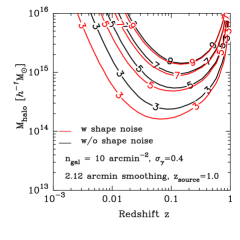
Figure 1: The effective selection function of galaxy clusters. Black line shows the expected convergence signal caused by an isolated dark matter halo. Red line shows the modulated peak height on a noisy smoothed convergence map (see the text for the definition). We plot each line in units of the variance of shape noise $\sigma_{\rm noise,0}=0.017$.

We adopt $\sigma_{\gamma}=0.4$, $n_{\rm gal}=10\,{\rm arcmin}^{-2}$ and the source redshift is set to be $z_{\rm source}=1$. These are the typical values for ground-based galaxy imaging surveys (e.g., Heymans et al., 2012). Also, we employ a Gaussian smoothing with the full width at half maximum of 5 arcmin. This corresponds to $\theta_{G}=5/\sqrt{8\ln 2}=2.12$ arcmin and thus to $\sigma_{\rm noise,0}\simeq 0.017$. Although the smoothing scale adopted here is slightly larger than that in previous works (see, e.g., Hamana, Takada & Yoshida, 2004) by a factor of about two, the noise level on the smoothed convergence map is similar. Gaussian smoothing with $\theta_{G}\sim 2$ arcmin with the actual data set is already examined in Shan et al. (2012).

Let us examine the effect of shape noise on weak lensing peaks. For this purpose, we define the mean modulation of peak height in a noisy ${\cal K}$ map as follows:

$${\bar{\cal K}}_{\rm peak,obs}(z,M)=\int{\rm d}{\cal K}\,{\cal K}\,{\rm Prob}({\cal K}|{\cal K}_{{\rm peak},h}(z,M)).$$ (28)

Figure 1 shows the comparison with ${\bar{\cal K}}_{\rm peak,obs}(z,M)$ and ${\cal K}_{{\rm peak},h}(z,M)$ for a given dark matter halo with mass of $M$ at redshift $z$. In this figure, red line shows the contour of ${\bar{\cal K}}_{\rm peak,obs}(z,M)$ in units of $\sigma_{\rm noise,0}$, whereas black line indicates the contour of ${\cal K}_{{\rm peak},h}(z,M)$. In a noisy $\cal K$ map, the shape noise modulates the height of peaks and the number of peaks slightly increases. We have tested the validity of our model against numerical simulations. The result is shown in Appendix A.

As shown in Figure 1, the Gaussian smoothing of $\sim 2$ arcmin are effective to search for clusters with mass of $\sim 10^{14}h^{-1}M_{\odot}$ at $z\sim 0.1-0.2$. The selection of mass and redshift is basically determined by the typical angular size of dark matter halos of interest (e.g., Hamana, Takada & Yoshida, 2004). Naively, it is expected that lower redshift clusters are detected with larger smoothing scales. In order to verify this expectation, we have studied the statistical properties of lensing peaks when adopting a Gaussian smoothing with the full width at half maximum of 15 arcmin (corresponding to $\theta_{G}\sim 6.4$ arcmin). In this case, we do not find one-to-one correspondence between selected peaks and halos, and thus our analytic model does not work. This is likely caused by the so-called projection effect; the effective redshift of lensing in the case of $z_{\rm source}=1$ is $0.1-0.5$ whereas we attempt to search for clusters at lower redshift $z<0.1$. We argue that our model is valid when the smoothing scale is set to be $1-2$ arcmin, corresponding to the typical angular size of dark matter halos with mass of $\sim 10^{14}h^{-1}M_{\odot}$ at $z\sim 0.1-0.5$.

2.3 Statistics

We consider a set of statistics derived from weak lensing measurement. In order to extract cosmological information from the number and the distribution of massive dark matter halos, we utilize peaks on a smoothed lensing map as described in Section 2.2.

Convergence power spectrum

First, we consider the power spectrum of convergence. Under the flat sky approximation, the Fourier transform of convergence field is defined by

$$\kappa(\mbox{\boldmath$\theta$})=\int\frac{{\rm d}^{2}\ell}{(2\pi)^{2}}e^{i\mbox{\boldmath$\ell$}\cdot\mbox{\boldmath$\theta$}}\tilde{\kappa}(\mbox{\boldmath$\ell$}).$$ (29)

The power spectrum of convergence field $P_{\kappa\kappa}$ is defined by

$$\langle\tilde{\kappa}(\mbox{\boldmath$\ell$}_{1})\tilde{\kappa}(\mbox{\boldmath$\ell$}_{2})\rangle=(2\pi)^{2}\delta_{D}^{(2)}(\mbox{\boldmath$\ell$}_{1}-\mbox{\boldmath$\ell$}_{2})P_{\kappa\kappa}(\ell_{1}),$$ (30)

where $\delta_{D}^{(2)}(\mbox{\boldmath$\ell$})$ is the Dirac delta function. By using Limber approximation (Limber, 1954; Kaiser, 1992) and Eq. (7), one can calculate the convergence power spectrum as follows:

$$P_{\kappa\kappa}(\ell) = \int_{0}^{\chi_{s}}{\rm d}\chi\frac{W_{\kappa}(\chi)^{2}}{r(\chi)^{2}}P_{\delta}\left(k=\frac{\ell}{r(\chi)},z(\chi)\right),$$ (31)

where $P_{\delta}(k)$ is the three dimensional matter power spectrum, $\chi_{s}$ is comoving distance to source galaxies and $W_{\kappa}(\chi)$ is the lensing weight function defined as

$$W_{\kappa}(\chi)=\frac{3}{2}\left(\frac{H_{0}}{c}\right)^{2}\Omega_{\rm m0}\frac{r(\chi_{s}-\chi)r(\chi)}{r(\chi_{s})}(1+z(\chi)).$$ (32)

The non-linear gravitational growth of density fluctuations significantly affects the amplitude of convergence power spectrum at the angular scales less than 1 degree (Jain, Seljak & White, 2000; Hilbert et al., 2009; Sato et al., 2009). Typical weak lensing surveys aim at measuring the angular scales larger than a few arcmin corresponding to a few Mpc. This leads weak lensing can be one of the most powerful probes for constraints on dark matter distribution at Mpc scale. Therefore, accurate theoretical prediction of non-linear matter power spectrum is essential for deriving cosmological constraints from weak lensing power spectrum. In order to predict the non-linear evolution of $P_{\delta}(k)$ for standard $\Lambda$CDM universe, a numerical approach based on $N$-body simulations has given steady results over the past few decades (Peacock & Dodds, 1996; Smith et al., 2003; Heitmann et al., 2010; Takahashi et al., 2012). We adopt the most recent model of non-linear $P_{\delta}(k)$ of Takahashi et al. (2012).

Convergence peak count

The number count of massive clusters is sensitive to various cosmological parameters such as the equation of state of dark energy (e.g., Allen, Evrard & Mantz, 2011). In this section, we use peak counts as a cosmological probe. We locate the local maxima in a smoothed lensing map and associate each identified peak with a massive dark matter halo along the same line of sight.

In practice, one can select a lensing peak by its peak height. We define the signal-to-noise ratio of a peak by $\nu={\cal K}_{\rm peak,obs}/\sigma_{\rm noise,0}$. For a given threshold $\nu_{\rm thre}$, one can predict the surface number density of peaks with $\nu>\nu_{\rm thre}$ as follows (e.g., Hamana, Takada & Yoshida, 2004):

$$N_{\rm peak}(\nu_{\rm thre})=\int{\rm d}z\,{\rm d}M\,\frac{{\rm d}^{2}V}{{\rm d}z{\rm d}\Omega}\frac{{\rm d}n}{{\rm d}M}(z,M)\int_{\nu_{\rm thre}\sigma_{\rm noise,0}}^{\infty}{\rm d}{\cal K}_{\rm peak,obs}\,\,{\rm Prob}({\cal K}_{\rm peak,obs}|\,{\cal K}_{{\rm peak},h}(z,M)),$$ (33)

where ${\rm d}n/{\rm d}M$ represents the mass function of dark matter halo and the volume element is expressed as ${\rm d}^{2}V/{\rm d}z{\rm d}\Omega=\chi^{2}/H(z)$ for a spatially flat universe. Here, ${\rm Prob}({\cal K}_{\rm peak,obs}|\,{\cal K}_{{\rm peak},h})$ is given by Eq. (23). In the following, we adopt the model of halo mass function in Bhattacharya et al. (2011).

Convergence peak auto spectrum and cross spectrum

We next consider the auto-correlation function of peaks, and the peak-convergence cross correlation. Marian et al. (2013) study cosmological information obtained from the statistics using a large set of numerical simulations. They conclude that using the auto- and cross-correlation functions can improve the constraints on cosmological parameters when combined with the number of peaks. We develop an analytic halo model in order to predict the correlation function of peaks and cross correlation between peaks and convergence.

In the halo model, the number density field of weak lensing selected clusters is given by

$$n_{\rm cl}(\mbox{\boldmath$x$}) = \sum_{i}\delta_{D}^{(3)}(\mbox{\boldmath$x$}-\mbox{\boldmath$x$}_{i})S(z_{i},M_{i})$$ (34)

$$= \sum_{i}\int{\rm d}M\,S(z,M)\,\delta_{D}(M-M_{i})\int{\rm d}^{3}\mbox{\boldmath$x$}^{\prime}\,\delta_{D}^{(3)}(\mbox{\boldmath$x$}^{\prime}-\mbox{\boldmath$x$}_{i})\delta_{D}^{(3)}(\mbox{\boldmath$x$}-\mbox{\boldmath$x$}^{\prime}),$$

where $S(z,M)$ represents the selection function (e.g., Takada & Bridle, 2007). For clusters identified as lensing peaks, $S(z,M)$ is expressed as

$$S(z,M|\nu_{\rm thre})=\int_{\nu_{\rm thre}\sigma_{\rm noise,0}}^{\infty}{\rm d}{\cal K}_{\rm peak,obs}\,\,{\rm Prob}({\cal K}_{\rm peak,obs}|\,{\cal K}_{{\rm peak},h}(z,M)).$$ (35)

Also, underlying matter density field can be approximated as

$$\rho_{m}(\mbox{\boldmath$x$}) = \sum_{i}\rho_{h}(\mbox{\boldmath$x$}-\mbox{\boldmath$x$}_{i}|z,M)$$ (36)

$$= \sum_{i}\int{\rm d}M\,M\,\delta_{D}(M-M_{i})\int{\rm d}^{3}\mbox{\boldmath$x$}^{\prime}\,\delta_{D}^{(3)}(\mbox{\boldmath$x$}^{\prime}-\mbox{\boldmath$x$}_{i})u_{m}(\mbox{\boldmath$x$}-\mbox{\boldmath$x$}^{\prime}|z,M),$$

where $\rho_{h}$ is the density profile of a massive halo given by Eq. (13), and $\rho_{h}(r|z,M)=Mu_{m}(r|z,M)$.

In order to derive the auto power spectrum of weak lensing selected clusters for a given threshold $\nu_{\rm thre}$, we first consider the auto power spectrum of $n_{\rm cl}$. The two point correlation function of $n_{\rm cl}$ is given by

$$\bar{n}_{\rm cl}^{2}\xi_{cc}(\mbox{\boldmath$x$}_{1}-\mbox{\boldmath$x$}_{2}) \equiv \langle n_{\rm cl}(\mbox{\boldmath$x$}_{1})n_{\rm cl}(\mbox{\boldmath$x$}_{1})\rangle-\bar{n}_{\rm cl}^{2}$$ (37)

$$= \langle\sum_{i}S^{2}(M_{i})\delta_{D}^{(3)}(\mbox{\boldmath$x$}_{1}-\mbox{\boldmath$x$}_{i})\delta_{D}^{(3)}(\mbox{\boldmath$x$}_{2}-\mbox{\boldmath$x$}_{i})\rangle+\langle\sum_{i,j|\,i\neq j}S(M_{i})S(M_{j})\delta_{D}^{(3)}(\mbox{\boldmath$x$}_{1}-\mbox{\boldmath$x$}_{i})\delta_{D}^{(3)}(\mbox{\boldmath$x$}_{2}-\mbox{\boldmath$x$}_{j})\rangle$$

$$= \langle\sum_{i}\int{\rm d}M\,\int{\rm d}^{3}y\,S^{2}(M)\delta_{D}(M-M_{i})\delta_{D}^{(3)}(\mbox{\boldmath$x$}_{1}-\mbox{\boldmath$y$})\delta_{D}^{(3)}(\mbox{\boldmath$x$}_{2}-\mbox{\boldmath$y$})\delta_{D}^{(3)}(\mbox{\boldmath$y$}-\mbox{\boldmath$x$}_{i})\rangle$$

$$+ \langle\sum_{i,j|\,i\neq j}\int{\rm d}M\,\int{\rm d}^{3}y\,S(M)\delta_{D}(M-M_{i})\delta_{D}^{(3)}(\mbox{\boldmath$x$}_{1}-\mbox{\boldmath$y$})\delta_{D}^{(3)}(\mbox{\boldmath$y$}-\mbox{\boldmath$x$}_{i})$$

$$\,\,\,\,\,\,\,\,\,\,\,\,\,\,\,\,\,\,\,\,\,\,\,\,\,\,\,\,\,\,\times\int{\rm d}M^{\prime}\,\int{\rm d}^{3}y^{\prime}\,S(M)\delta_{D}(M^{\prime}-M_{j})\delta_{D}^{(3)}(\mbox{\boldmath$x$}_{2}-\mbox{\boldmath$y$}^{\prime})\delta_{D}^{(3)}(\mbox{\boldmath$y$}^{\prime}-\mbox{\boldmath$x$}_{j})\rangle$$

$$= \int{\rm d}M\,\frac{{\rm d}n}{{\rm d}M}S^{2}(M)\int{\rm d}^{3}y\,\delta_{D}^{(3)}(\mbox{\boldmath$x$}_{1}-\mbox{\boldmath$y$})\delta_{D}^{(3)}(\mbox{\boldmath$x$}_{2}-\mbox{\boldmath$y$})$$

$$+ \int{\rm d}M\,\frac{{\rm d}n}{{\rm d}M}S(M)\int{\rm d}^{3}y\,\delta_{D}^{(3)}(\mbox{\boldmath$x$}_{1}-\mbox{\boldmath$y$})\int{\rm d}M^{\prime}\,\frac{{\rm d}n}{{\rm d}M^{\prime}}S(M^{\prime})\int{\rm d}^{3}y^{\prime}\,\delta_{D}^{(3)}(\mbox{\boldmath$x$}_{2}-\mbox{\boldmath$y$}^{\prime})\xi_{hh}(\mbox{\boldmath$y$}-\mbox{\boldmath$y$}^{\prime};M,M^{\prime})$$

$$= \int{\rm d}M\,\frac{{\rm d}n}{{\rm d}M}S^{2}(M)\int{\rm d}^{3}y\,\delta_{D}^{(3)}(\mbox{\boldmath$x$}_{1}-\mbox{\boldmath$x$}_{2})+\int{\rm d}M\,\frac{{\rm d}n}{{\rm d}M}S(M)\int{\rm d}M^{\prime}\,\frac{{\rm d}n}{{\rm d}M^{\prime}}S(M^{\prime})\xi_{hh}(\mbox{\boldmath$x$}_{1}-\mbox{\boldmath$x$}_{2};M,M^{\prime}),$$

where $\xi_{hh}(\mbox{\boldmath$y$}-\mbox{\boldmath$y$}^{\prime};M,M^{\prime})$ is the two point correlation function of dark matter haloes with mass of $M$ and $M^{\prime}$. In the above calculation, we use the following relations as

$$\langle\sum_{i}\delta_{D}(M-M_{i})\delta_{D}^{(3)}(\mbox{\boldmath$x$}-\mbox{\boldmath$x$}_{i})\rangle \equiv \frac{{\rm d}n}{{\rm d}M},$$ (38)

$$\langle\sum_{i,j|\,i\neq j}\delta_{D}(M-M_{i})\delta_{D}(M^{\prime}-M_{j})\delta_{D}^{(3)}(\mbox{\boldmath$x$}_{1}-\mbox{\boldmath$x$}_{i})\delta_{D}^{(3)}(\mbox{\boldmath$x$}_{2}-\mbox{\boldmath$x$}_{j})\rangle \equiv \frac{{\rm d}n}{{\rm d}M}\frac{{\rm d}n}{{\rm d}M^{\prime}}\xi_{hh}(\mbox{\boldmath$x$}_{1}-\mbox{\boldmath$x$}_{2}^{\prime};M,M^{\prime}).$$ (39)

We further approximate $\xi_{hh}$ as $b_{h}(M)b_{h}(M^{\prime})\xi_{\delta\delta}^{L}$, where $b_{h}$ is the linear halo bias and $\xi_{\delta\delta}^{L}$ is the two point correlation function of linear matter density field. Then, we finally obtain the following equation:

$$\bar{n}_{\rm cl}^{2}\xi_{cc}(\mbox{\boldmath$x$}_{1}-\mbox{\boldmath$x$}_{2}) = \int{\rm d}M\,\frac{{\rm d}n}{{\rm d}M}\,S^{2}(M)\delta_{D}^{(3)}(\mbox{\boldmath$x$}_{1}-\mbox{\boldmath$x$}_{2})+\left[\int\,{\rm d}M\,\frac{{\rm d}n}{{\rm d}M}\,S(M)b_{h}(M)\right]^{2}\xi_{\delta\delta}^{L}(\mbox{\boldmath$x$}_{1}-\mbox{\boldmath$x$}_{2}).$$ (40)

The Fourier transform of Eq. (40) is the three-dimensional power spectrum of $n_{cl}$, which is expressed as

$$P_{cc}(k)=\int{\rm d}^{3}r\,e^{-i\mbox{\boldmath$k$}\cdot\mbox{\boldmath$r$}}\xi_{cc}(r).$$ (41)

The observed surface number density of weak lensing selected clusters (for a given threshold $\nu_{\rm thre}$) is thus given by

$$p(\mbox{\boldmath$\theta$})=\frac{1}{N_{\rm peak}(\nu_{\rm thre})}\int{\rm d}\chi\,\frac{{\rm d}^{2}V}{{\rm d}\chi{\rm d}\Omega}n_{\rm cl}(r(\chi)\mbox{\boldmath$\theta$},z(\chi)),$$ (42)

where $N_{\rm peak}$ is defined by Eq. (33). Using the Limber approximation, we can derive the angular power spectrum of $p$ as

$$P_{\rm pp}(\ell) = \int{\rm d}\chi\,\frac{1}{r(\chi)^{2}}\left(\frac{1}{N_{\rm peak}}\frac{{\rm d}^{2}V}{{\rm d}\chi{\rm d}\Omega}\right)^{2}\bar{n}_{\rm cl}^{2}P_{cc}\left(k=\frac{\ell}{r(\chi)},z(\chi)\right).$$ (43)

Except for the shot noise term in Eq. (48), we obtain

$$P_{\rm pp}(\ell)=\int{\rm d}\chi\,\frac{1}{r(\chi)^{2}}\left(\frac{1}{N_{\rm peak}}\frac{{\rm d}^{2}V}{{\rm d}\chi{\rm d}\Omega}\right)^{2}\left[\int{\rm d}M\,\frac{{\rm d}n}{{\rm d}M}(z,M)S(z,M|\nu_{\rm thre})b_{h}(z,M)\right]^{2}\,P^{L}_{m}\left(k=\frac{\ell}{r(\chi)},z(\chi)\right),$$ (44)

where $P^{L}_{m}$ is the linear matter power spectrum. Throughput this paper, we adopt the functional form of $b_{h}$ proposed in Bhattacharya et al. (2011).

The similar derivation can be applied to the cross power spectrum of weak lensing selected clusters and lensing convergence. Let us first consider the three-dimensional cross correlation function of $n_{\rm cl}$ and $\rho_{m}$:

$$\bar{\rho}_{m}\xi_{c\delta}(\mbox{\boldmath$x$}_{1}-\mbox{\boldmath$x$}_{2}) = \langle n_{\rm cl}(\mbox{\boldmath$x$}_{1})\rho_{m}(\mbox{\boldmath$x$}_{1})\rangle-\bar{n}_{\rm cl}\bar{\rho}_{m}$$ (45)

$$= \int{\rm d}M\,\frac{{\rm d}n}{{\rm d}M}\,S(M)Mu_{m}(\mbox{\boldmath$x$}_{1}-\mbox{\boldmath$x$}_{2}|M)+\left[\int\,{\rm d}M\,\frac{{\rm d}n}{{\rm d}M}\,S(M)b_{h}(M)\right]\bar{\rho}_{m}\xi_{\delta\delta}^{L}(\mbox{\boldmath$x$}_{1}-\mbox{\boldmath$x$}_{2}).$$

Through the derivation of Eq. (45), we use the following fact that

$$\bar{\rho}_{m}=\int{\rm d}M\,\frac{{\rm d}n}{{\rm d}M}\,b_{h}(M)M\int{\rm d}^{3}x^{\prime}\,u_{m}(\mbox{\boldmath$x$}-\mbox{\boldmath$x$}^{\prime}|M).$$ (46)

Then, we can obtain the angular cross power spectrum of $p$ and lensing convergence $\kappa$ by the similar calculation as Eq. (43). The cross power spectrum $P_{{\rm p}\kappa}$ is given by

$$P_{{\rm p}\kappa}(\ell)=\int{\rm d}\chi\,\frac{W_{\kappa}(\chi)}{r(\chi)^{2}}\left(\frac{1}{N_{\rm peak}}\frac{{\rm d}^{2}V}{{\rm d}\chi{\rm d}\Omega}\right)P_{c\delta}\left(k=\frac{\ell}{r(\chi)},z(\chi)\right),$$ (47)

where $P_{c\delta}(k)$ represents the three-dimensional cross power spectrum of $n_{\rm cl}$ and matter overdensity field $\delta$, i.e.,

$$P_{c\delta}(k)=\int{\rm d}^{3}r\,e^{-i\mbox{\boldmath$k$}\cdot\mbox{\boldmath$r$}}\xi_{c\delta}(r).$$ (48)

Finally, the cross power spectrum between peaks and convergence is given by (also, see Oguri & Takada (2011))

$$P_{{\rm p}\kappa}(\ell) = P^{1h}_{{\rm p}\kappa}(\ell)+P^{2h}_{{\rm p}\kappa}(\ell),$$ (49)

$$P^{1h}_{{\rm p}\kappa}(\ell) = \int{\rm d}\chi\,\frac{W_{\kappa}(\chi)}{r(\chi)^{2}}\left(\frac{1}{N_{\rm peak}}\frac{{\rm d}^{2}V}{{\rm d}\chi{\rm d}\Omega}\right)\int{\rm d}M\,\frac{{\rm d}n}{{\rm d}M}S(z,M|\nu_{\rm thre})\,\left(\frac{M}{\bar{\rho}_{m}(z)}\right)\tilde{u}_{m}\left(k=\frac{\ell}{r(\chi)}\Bigg{|}z(\chi),M\right),$$ (50)

$$P^{2h}_{{\rm p}\kappa}(\ell) = \int{\rm d}\chi\,\frac{W_{\kappa}(\chi)}{r(\chi)^{2}}\left(\frac{1}{N_{\rm peak}}\frac{{\rm d}^{2}V}{{\rm d}\chi{\rm d}\Omega}\right)\left[\int{\rm d}M\,\frac{{\rm d}n}{{\rm d}M}(z,M)S(z,M|\nu_{\rm thre})b_{h}(z,M)\right]\,P^{L}_{m}\left(k=\frac{\ell}{r(\chi)},z(\chi)\right),$$ (51)

where $\tilde{u}_{m}$ is the Fourier transform of $u_{m}(r|z,M)$.

2.4 Covariances between statistics

We summarize covariance matrices between statistics of interest in the following. As a first approximation, we can use the Gaussian covariance between three binned spectra $P_{\kappa\kappa}$, $P_{{\rm p}\kappa}$ and $P_{\rm pp}$ as,

$${\rm Cov}[P_{XY}(\ell),P_{AB}(\ell^{\prime})]=\frac{1}{(2\ell+1)\Delta\ell f_{\rm sky}}\left[P^{\rm obs}_{XA}(\ell)P^{\rm obs}_{YB}(\ell)+P^{\rm obs}_{XB}(\ell)P^{\rm obs}_{YA}(\ell)\right]\delta_{\ell\ell^{\prime}},$$ (52)

where $\Delta\ell$ is the width of binning in multipole and $f_{\rm sky}$ represents the observed sky fraction. The observed spectra $P^{\rm obs}_{XY}(\ell)$ are then defined by

$$P^{\rm obs}_{\kappa\kappa}=P_{\kappa\kappa}+\frac{\sigma_{\gamma}^{2}}{2n_{\rm gal}},\,P^{\rm obs}_{\rm pp}=P_{\rm pp}+\frac{1}{N_{\rm peak}},\,P^{\rm obs}_{{\rm p}\kappa}=P_{{\rm p}\kappa}.$$ (53)

The non-linear gravitational growth causes mode-coupling of the density fluctuations with different wavelengths. The mode-coupling then induces the correlation of weak lensing statistics between different multipoles, i.e., we can not use the Gaussian approximation to covariances (e.g., Sato et al., 2009). Modeling of the non-Gaussian covariances is still being developed (e.g., Cooray & Hu, 2001; Takada & Jain, 2004; Takada & Bridle, 2007). We here present a theoretical model of non-Gaussian covariance matrices between $P_{\kappa\kappa}$, $P_{{\rm p}\kappa}$ and $N_{\rm peak}$.

Let us consider the following set of four-point correlation functions in Fourier space:

$$\langle\tilde{\delta}_{m}(\mbox{\boldmath$k$}_{1})\tilde{\delta}_{m}(\mbox{\boldmath$k$}_{2})\tilde{\delta}_{m}(\mbox{\boldmath$k$}_{3})\tilde{\delta}_{m}(\mbox{\boldmath$k$}_{4})\rangle = (2\pi)^{3}\delta^{(3)}_{D}(\mbox{\boldmath$k$}_{1234})T_{\delta\delta\delta\delta}(\mbox{\boldmath$k$}_{1},\mbox{\boldmath$k$}_{2},\mbox{\boldmath$k$}_{3},\mbox{\boldmath$k$}_{4})$$ (54)

$$\langle\tilde{\delta}_{cl}(\mbox{\boldmath$k$}_{1})\tilde{\delta}_{m}(\mbox{\boldmath$k$}_{2})\tilde{\delta}_{cl}(\mbox{\boldmath$k$}_{3})\tilde{\delta}_{m}(\mbox{\boldmath$k$}_{4})\rangle = (2\pi)^{3}\delta^{(3)}_{D}(\mbox{\boldmath$k$}_{1234})T_{c\delta c\delta}(\mbox{\boldmath$k$}_{1},\mbox{\boldmath$k$}_{2},\mbox{\boldmath$k$}_{3},\mbox{\boldmath$k$}_{4})$$ (55)

$$\langle\tilde{\delta}_{cl}(\mbox{\boldmath$k$}_{1})\tilde{\delta}_{m}(\mbox{\boldmath$k$}_{2})\tilde{\delta}_{m}(\mbox{\boldmath$k$}_{3})\tilde{\delta}_{m}(\mbox{\boldmath$k$}_{4})\rangle = (2\pi)^{3}\delta^{(3)}_{D}(\mbox{\boldmath$k$}_{1234})T_{c\delta\delta\delta}(\mbox{\boldmath$k$}_{1},\mbox{\boldmath$k$}_{2},\mbox{\boldmath$k$}_{3},\mbox{\boldmath$k$}_{4}),$$ (56)

where $\mbox{\boldmath$k$}_{ij\cdots n}=\mbox{\boldmath$k$}_{i}+\mbox{\boldmath$k$}_{j}+\cdots+\mbox{\boldmath$k$}_{n}$, $\delta_{m}$ and $\delta_{cl}$ represent over density of matter and weak lensing selected clusters, respectively. In the flat sky approximation, we can relate three tri-spectra $(T_{\delta\delta\delta\delta},T_{c\delta c\delta},T_{c\delta\delta\delta})$ with the non-Gaussian part of the covariance matrix of weak lensing statistics as follows:

$${\rm Cov}\left[P_{\kappa\kappa}(\ell),P_{\kappa\kappa}(\ell^{\prime})\right]_{\rm NG} = \frac{1}{4\pi}\int\frac{{\rm d}\phi}{2\pi}T_{\kappa\kappa\kappa\kappa}(\mbox{\boldmath$\ell$},-\mbox{\boldmath$\ell$},\mbox{\boldmath$\ell$}^{\prime},-\mbox{\boldmath$\ell$}^{\prime};\phi),$$ (57)

$${\rm Cov}\left[P_{{\rm p}\kappa}(\ell),P_{{\rm p}\kappa}(\ell^{\prime})\right]_{\rm NG} = \frac{1}{4\pi}\int\frac{{\rm d}\phi}{2\pi}T_{{\rm p}\kappa{\rm p}\kappa}(\mbox{\boldmath$\ell$},-\mbox{\boldmath$\ell$},\mbox{\boldmath$\ell$}^{\prime},-\mbox{\boldmath$\ell$}^{\prime};\phi),$$ (58)

$${\rm Cov}\left[P_{{\rm p}\kappa}(\ell),P_{\kappa\kappa}(\ell^{\prime})\right]_{\rm NG} = \frac{1}{4\pi}\int\frac{{\rm d}\phi}{2\pi}T_{{\rm p}\kappa\kappa\kappa}(\mbox{\boldmath$\ell$},-\mbox{\boldmath$\ell$},\mbox{\boldmath$\ell$}^{\prime},-\mbox{\boldmath$\ell$}^{\prime};\phi),$$ (59)

where $\phi$ is the angle between two vectors $\ell$ and $\mbox{\boldmath$\ell$}^{\prime}$. In practice, the integral over $\phi$ is often simplified as, e.g.,

$$\frac{1}{4\pi}\int\frac{{\rm d}\phi}{2\pi}T_{\kappa\kappa\kappa\kappa}(\mbox{\boldmath$\ell$},-\mbox{\boldmath$\ell$},\mbox{\boldmath$\ell$}^{\prime},-\mbox{\boldmath$\ell$}^{\prime};\phi)\simeq T_{\kappa\kappa\kappa\kappa}(\ell,\ell,\ell^{\prime},{\ell}^{\prime}),$$ (60)

and so on. With Limber approximation, $T_{\kappa\kappa\kappa\kappa}$, $T_{{\rm p}\kappa{\rm p}\kappa}$, and $T_{{\rm p}\kappa\kappa\kappa}$ are given by

$$T_{\kappa\kappa\kappa\kappa}(\mbox{\boldmath$\ell$}_{1},\mbox{\boldmath$\ell$}_{2},\mbox{\boldmath$\ell$}_{3},\mbox{\boldmath$\ell$}_{4}) = \int_{0}^{\chi_{s}}{\rm d}\chi\,\frac{W_{\kappa}^{4}}{r(\chi)^{6}}T_{\delta\delta\delta\delta}(\mbox{\boldmath$k$}_{1},\mbox{\boldmath$k$}_{2},\mbox{\boldmath$k$}_{3},\mbox{\boldmath$k$}_{4};z(\chi)),$$ (61)

$$T_{{\rm p}\kappa{\rm p}\kappa}(\mbox{\boldmath$\ell$}_{1},\mbox{\boldmath$\ell$}_{2},\mbox{\boldmath$\ell$}_{3},\mbox{\boldmath$\ell$}_{4}) = \int_{0}^{\chi_{s}}{\rm d}\chi\,\frac{W_{\kappa}^{2}}{r(\chi)^{6}}\left(\frac{1}{N_{\rm peak}}\frac{{\rm d}^{2}V}{{\rm d}\chi{\rm d}\Omega}\right)^{2}T_{c\delta c\delta}(\mbox{\boldmath$k$}_{1},\mbox{\boldmath$k$}_{2},\mbox{\boldmath$k$}_{3},\mbox{\boldmath$k$}_{4};z(\chi)),$$ (62)

$$T_{{\rm p}\kappa\kappa\kappa}(\mbox{\boldmath$\ell$}_{1},\mbox{\boldmath$\ell$}_{2},\mbox{\boldmath$\ell$}_{3},\mbox{\boldmath$\ell$}_{4}) = \int_{0}^{\chi_{s}}{\rm d}\chi\,\frac{W_{\kappa}^{3}}{r(\chi)^{6}}\left(\frac{1}{N_{\rm peak}}\frac{{\rm d}^{2}V}{{\rm d}\chi{\rm d}\Omega}\right)T_{c\delta\delta\delta}(\mbox{\boldmath$k$}_{1},\mbox{\boldmath$k$}_{2},\mbox{\boldmath$k$}_{3},\mbox{\boldmath$k$}_{4};z(\chi)),$$ (63)

where $k_{i}=l_{i}/\chi$, $\chi_{s}$ is the comoving distance to sources, the window function $W_{\kappa}$ is given by Eq. (32) and $N_{\rm peak}$ is defined by Eq. (33).

Previous works show that the dominant contribution of the non-Gaussian covariance is the so-called one-halo term of the relevant tri-spectrum at $\ell\lower 2.15277pt\hbox{$\;\buildrel>\over{\sim}\;$}100$ (e.g., Sato et al., 2009). One halo term arises from the four point correlation between different modes $\mbox{\boldmath$k$}_{i}\,(i=1,2,3,4)$ in a single dark matter halo. Thus, one halo term of the underlying tri-spectra between $\delta_{m}$ and $\delta_{c}$ can be calculated as

$$T_{\delta\delta\delta\delta}^{1h}(\mbox{\boldmath$k$}_{1},\mbox{\boldmath$k$}_{2},\mbox{\boldmath$k$}_{3},\mbox{\boldmath$k$}_{4};z) = \int{\rm d}M\,\frac{{\rm d}n}{{\rm d}M}(z,M)\,\left(\frac{M}{\bar{\rho}_{m}(z)}\right)^{4}\tilde{u}_{m}(\mbox{\boldmath$k$}_{1}|z,M)\tilde{u}_{m}(\mbox{\boldmath$k$}_{2}|z,M)\tilde{u}_{m}(\mbox{\boldmath$k$}_{3}|z,M)\tilde{u}_{m}(\mbox{\boldmath$k$}_{4}|z,M),$$ (64)

$$T_{c\delta c\delta}^{1h}(\mbox{\boldmath$k$}_{1},\mbox{\boldmath$k$}_{2},\mbox{\boldmath$k$}_{3},\mbox{\boldmath$k$}_{4};z) = \int{\rm d}M\,\frac{{\rm d}n}{{\rm d}M}(z,M)\,\left(\frac{M}{\bar{\rho}_{m}(z)}\right)^{2}S(z,M)\tilde{u}_{m}(\mbox{\boldmath$k$}_{2}|z,M)\tilde{u}_{m}(\mbox{\boldmath$k$}_{4}|z,M),$$ (65)

$$T_{c\delta\delta\delta}^{1h}(\mbox{\boldmath$k$}_{1},\mbox{\boldmath$k$}_{2},\mbox{\boldmath$k$}_{3},\mbox{\boldmath$k$}_{4};z) = \int{\rm d}M\,\frac{{\rm d}n}{{\rm d}M}(z,M)\,\left(\frac{M}{\bar{\rho}_{m}(z)}\right)^{3}S(z,M)\tilde{u}_{m}(\mbox{\boldmath$k$}_{2}|z,M)\tilde{u}_{m}(\mbox{\boldmath$k$}_{3}|z,M)\tilde{u}_{m}(\mbox{\boldmath$k$}_{4}|z,M).$$ (66)

Another important contribution of covariance at degree scales or less is so-called halo sampling variance (HSV) (Sato et al., 2009; Kayo, Takada & Jain, 2013). This term describes the mode-coupling between the measured Fourier modes and larger modes of length-scales comparable to survey volume. It is expected to be important when the number of massive haloes found in a finite region is correlated with the overall mass density fluctuation in the region (Hu & Kravtsov, 2003). Following Kayo, Takada & Jain (2013), we model the HSV of weak lensing statistics as

$${\rm Cov}\left[P_{\kappa\kappa}(\ell),P_{\kappa\kappa}(\ell^{\prime})\right]_{\rm HSV} = \int_{0}^{\chi_{s}}{\rm d}\chi\,\left(\frac{{\rm d}^{2}V}{{\rm d}\chi{\rm d}\Omega}\right)^{2}\,\left[\int{\rm d}M\,\frac{{\rm d}n}{{\rm d}M}b_{h}(M)|\tilde{\kappa}_{h}(\ell|M)|^{2}\right]$$ (67)

$$\times \left[\int{\rm d}M^{\prime}\,\frac{{\rm d}n}{{\rm d}M^{\prime}}b_{h}(M^{\prime})|\tilde{\kappa}_{h}(\ell^{\prime}|M^{\prime})|^{2}\right]\left[\int_{0}^{\infty}\frac{k{\rm d}k}{2\pi}P^{L}_{m}(k)|\tilde{W}(k\chi\Theta_{\rm survey})|^{2}\right],$$

$${\rm Cov}\left[P_{{\rm p}\kappa}(\ell),P_{{\rm p}\kappa}(\ell^{\prime})\right]_{\rm HSV} = \int_{0}^{\chi_{s}}{\rm d}\chi\,\left(\frac{{\rm d}^{2}V}{{\rm d}\chi{\rm d}\Omega}\right)^{2}\,\left[\int{\rm d}M\,\frac{{\rm d}n}{{\rm d}M}b_{h}(M)S(z,M)\tilde{\kappa}_{h}(\ell|M)\right]$$ (68)

$$\times \left[\int{\rm d}M^{\prime}\,\frac{{\rm d}n}{{\rm d}M^{\prime}}b_{h}(M^{\prime})S(z,M^{\prime})\tilde{\kappa}_{h}(\ell^{\prime}|M^{\prime})\right]\left[\int_{0}^{\infty}\frac{k{\rm d}k}{2\pi}P^{L}_{m}(k)|\tilde{W}(k\chi\Theta_{\rm survey})|^{2}\right],$$

$${\rm Cov}\left[P_{{\rm p}\kappa}(\ell),P_{\kappa\kappa}(\ell^{\prime})\right]_{\rm HSV} = \int_{0}^{\chi_{s}}{\rm d}\chi\,\left(\frac{{\rm d}^{2}V}{{\rm d}\chi{\rm d}\Omega}\right)^{2}\,\left[\int{\rm d}M\,\frac{{\rm d}n}{{\rm d}M}b_{h}(M)S(z,M)\tilde{\kappa}_{h}(\ell|M)\right]$$ (69)

$$\times \left[\int{\rm d}M^{\prime}\,\frac{{\rm d}n}{{\rm d}M^{\prime}}b_{h}(M^{\prime})|\tilde{\kappa}_{h}(\ell^{\prime}|M^{\prime})|^{2}\right]\left[\int_{0}^{\infty}\frac{k{\rm d}k}{2\pi}P^{L}_{m}(k)|\tilde{W}(k\chi\Theta_{\rm survey})|^{2}\right],$$

where $\kappa_{h}$ is the Fourier transforming of Eq. (15). Here, $\tilde{W}(k\chi\Theta_{\rm survey})$ represents the window function of the survey region in Fourier space with $\Theta_{\rm survey}$ denoting the squared root of the survey area. We use the circular function of $\tilde{W}(x)=J_{1}(x)/x$.

Cross covariance between the number count of weak lensing selected clusters and the lensing spectra can be naturally incorporated in the halo model (Takada & Bridle, 2007; Takada & Spergel, 2014).

The covariance of $N_{\rm peak}$ with two different thresholds is given by

$${\rm Cov}[N_{\rm peak}(\nu_{{\rm thre},1}),N_{\rm peak}(\nu_{{\rm thre},2})] = \int{\rm d}^{2}\theta\,W({\mbox{\boldmath$\theta$}})\int{\rm d}\theta^{\prime}\,W({\mbox{\boldmath$\theta$}}^{\prime})\int{\rm d}\chi\,\frac{{\rm d}^{2}V}{{\rm d}\chi{\rm d}\Omega}\int{\rm d}\chi^{\prime}\,\frac{{\rm d}^{2}V}{{\rm d}\chi^{\prime}{\rm d}\Omega^{\prime}}$$ (70)

$$\times\left[n_{\rm cl}(\chi{\mbox{\boldmath$\theta$}},z(\chi)|\nu_{{\rm thre},1})n_{\rm cl}(\chi^{\prime}{\mbox{\boldmath$\theta$}}^{\prime},z(\chi^{\prime})|\nu_{{\rm thre},2})-\bar{n}_{\rm cl}(z(\chi)|\nu_{{\rm thre},1})\bar{n}_{\rm cl}(z(\chi^{\prime})|\nu_{{\rm thre},2})\right],$$

where $W({\mbox{\boldmath$\theta$}})$ represents the window function in real space. Performing the similar calculation as in Eq. (37), one can find that (see also the appendix in Takada & Bridle (2007))

$${\rm Cov}[N_{\rm peak}(\nu_{{\rm thre},1}),N_{\rm peak}(\nu_{{\rm thre},2})] = \delta_{12}\Biggl{\{}\frac{N_{\rm peak}(\nu_{{\rm thre},1})}{4\pi f_{\rm sky}}+\int{\rm d}\chi\,\left(\frac{{\rm d}^{2}V}{{\rm d}\chi{\rm d}\Omega}\right)^{2}\,r(\chi)^{-2}\,\left[\int{\rm d}M\,\frac{{\rm d}n}{{\rm d}M}b_{h}(M)S(z,M|\nu_{{\rm thre},1})\right]^{2}$$ (71)

$$\,\,\,\,\,\,\,\,\,\,\,\,\,\,\,\,\,\,\,\,\,\,\,\,\,\,\,\,\,\,\,\,\,\,\,\,\,\,\,\,\,\,\,\,\,\,\,\,\,\,\,\,\,\,\,\,\,\,\,\,\,\,\,\,\,\,\,\,\,\,\,\,\,\,\,\,\,\,\,\,\,\,\,\,\,\,\,\,\,\,\,\,\,\,\,\,\,\,\times\left[\int_{0}^{\infty}\frac{k{\rm d}k}{2\pi}P^{L}_{m}(k)|\tilde{W}(k\chi\Theta_{\rm survey})|^{2}\right]\Biggr{\}},$$

where $f_{\rm sky}$ is the sky fraction for survey of interest. In order to derive the cross covariance between $N_{\rm peak}$ and $P_{\kappa\kappa}$ or $P_{{\rm p}\kappa}$, we first define the estimator of power spectrum as

$$P_{\kappa\kappa}^{\rm est}(\ell)=\frac{1}{4\pi f_{\rm sky}N_{p}(\ell)}\sum_{{\mbox{\boldmath$\ell$}}}{\tilde{\kappa}}({\mbox{\boldmath$\ell$}}){\tilde{\kappa}}(-{\mbox{\boldmath$\ell$}}),\,\,\,P_{{\rm p}\kappa}^{\rm est}(\ell|\nu_{\rm thre})=\frac{1}{4\pi f_{\rm sky}N_{p}(\ell)}\sum_{{\mbox{\boldmath$\ell$}}}{\tilde{p}}({\mbox{\boldmath$\ell$}}|\nu_{\rm thre}){\tilde{\kappa}}(-{\mbox{\boldmath$\ell$}}),$$ (72)

where the summation is taken over all the Fourier modes in the range of $[\ell-\Delta\ell/2,\ell+\Delta\ell/2]$ and $\Delta\ell$ is the width of multipoles. Also, $N_{p}(\ell)$ represents the number of modes to estimate of power spectrum with the multipole of $\ell$. With Eq. (72), we can express the cross covariance of $N_{\rm peak}$ and $P_{\kappa\kappa}$ as

$${\rm Cov}[N_{\rm peak}(\nu_{\rm thre}),P_{\kappa\kappa}(\ell)] = \frac{1}{4\pi f_{\rm sky}N_{p}(\ell)}\sum_{\mbox{\boldmath$\ell$}}\int{\rm d}^{2}\theta\,W({\mbox{\boldmath$\theta$}})\langle{\tilde{\kappa}}({\mbox{\boldmath$\ell$}}){\tilde{\kappa}}(-{\mbox{\boldmath$\ell$}})\left[n_{\rm cl}(\chi{\mbox{\boldmath$\theta$}},z(\chi)|\nu_{{\rm thre}})-\bar{n}_{\rm cl}(z(\chi)|\nu_{\rm thre})\right]\rangle,$$ (73)

$$= \frac{1}{4\pi f_{\rm sky}N_{p}(\ell)}\int{\rm d}^{2}\theta\,W({\mbox{\boldmath$\theta$}})N_{\rm peak}(\nu_{\rm thre})\sum_{\mbox{\boldmath$\ell$}}\sum_{{\mbox{\boldmath$\ell$}}^{\prime}}\langle{\tilde{\kappa}}({\mbox{\boldmath$\ell$}}){\tilde{\kappa}}(-{\mbox{\boldmath$\ell$}}){\tilde{p}}({\mbox{\boldmath$\ell$}}^{\prime}|\nu_{\rm thre})\rangle e^{-i{\mbox{\boldmath$\ell$}}^{\prime}\cdot{\mbox{\boldmath$\theta$}}},$$

where we use Eq. (42) through the derivation. Similarly, the cross covariances of $N_{\rm peak}$ and $P_{{\rm p}\kappa}$ is given by

$${\rm Cov}[N_{\rm peak}(\nu_{{\rm thre},1}),P_{{\rm p}\kappa}(\ell|\nu_{{\rm thre},2})] = \frac{1}{4\pi f_{\rm sky}N_{p}(\ell)}\int{\rm d}^{2}\theta\,W({\mbox{\boldmath$\theta$}})N_{\rm peak}(\nu_{{\rm thre},2})$$ (74)

$$\,\,\,\,\,\,\,\,\,\,\,\,\,\,\,\,\,\,\,\,\,\,\,\,\,\,\,\,\,\,\,\,\,\,\,\,\,\,\,\,\,\,\,\,\,\,\,\,\,\,\,\,\,\,\,\,\,\,\,\,\,\,\,\,\,\,\,\,\,\,\times\sum_{\mbox{\boldmath$\ell$}}\sum_{{\mbox{\boldmath$\ell$}}^{\prime}}\langle{\tilde{p}}({\mbox{\boldmath$\ell$}}|\nu_{{\rm thre},1}){\tilde{\kappa}}(-{\mbox{\boldmath$\ell$}}){\tilde{p}}({\mbox{\boldmath$\ell$}}^{\prime}|\nu_{{\rm thre},2})\rangle e^{-i{\mbox{\boldmath$\ell$}}^{\prime}\cdot{\mbox{\boldmath$\theta$}}}.$$

Therefore, the cross covariances of $N_{\rm peak}$ and lensing spectra include the three point correlation of the relevant field $p$ or $\kappa$. We can thus summarize the relevant covariance are

$${\rm Cov}[N_{\rm peak}(\nu_{\rm thre}),P_{\kappa\kappa}(\ell)] = \frac{1}{4\pi f_{\rm sky}}\int{\rm d}\chi\,\frac{{\rm d}^{2}V}{{\rm d}\chi{\rm d}\Omega}\,\frac{W_{\kappa}^{2}}{r(\chi)^{4}}\,B_{c\delta\delta}(0,\ell/\chi,\ell/\chi;z(\chi)),$$ (75)

$${\rm Cov}[N_{\rm peak}(\nu_{{\rm thre},1}),P_{{\rm p}\kappa}(\ell|\nu_{{\rm thre},2})] = \frac{1}{4\pi f_{\rm sky}}\int{\rm d}\chi\,\left(\frac{{\rm d}^{2}V}{{\rm d}\chi{\rm d}\Omega}\right)^{2}\,\frac{W_{\kappa}}{r(\chi)^{4}}\,B_{c(1)c(2)\delta}(0,\ell/\chi,\ell/\chi;z(\chi)),$$ (76)

where $B_{c\delta\delta}$ and $B_{c(1)c(2)\delta}$ are defined by

$$\langle\tilde{\delta}_{cl}(\mbox{\boldmath$k$}_{1})\tilde{\delta}_{m}(\mbox{\boldmath$k$}_{2})\tilde{\delta}_{m}(\mbox{\boldmath$k$}_{3})\rangle = (2\pi)^{3}\delta^{(3)}_{D}(\mbox{\boldmath$k$}_{123})B_{c\delta\delta}({\mbox{\boldmath$k$}}_{1},{\mbox{\boldmath$k$}}_{2},{\mbox{\boldmath$k$}}_{3}),$$ (77)

$$\langle\tilde{\delta}_{cl}(\mbox{\boldmath$k$}_{1}|\nu_{{\rm thre},1})\tilde{\delta}_{cl}(\mbox{\boldmath$k$}_{2}|\nu_{{\rm thre},2})\tilde{\delta}_{m}(\mbox{\boldmath$k$}_{3})\rangle = (2\pi)^{3}\delta^{(3)}_{D}(\mbox{\boldmath$k$}_{123})B_{c(1)c(2)\delta}({\mbox{\boldmath$k$}}_{1},{\mbox{\boldmath$k$}}_{2},{\mbox{\boldmath$k$}}_{3}).$$ (78)

At $\ell\lower 2.15277pt\hbox{$\;\buildrel>\over{\sim}\;$}500$, the main contributor to the covariances is the one-halo term of the above bi-spectra. Similarly to the case of tri-spectra, the corresponding terms are expressed as

$$B_{c\delta\delta}^{1h}(\mbox{\boldmath$k$}_{1},\mbox{\boldmath$k$}_{2},\mbox{\boldmath$k$}_{3};z) = \int{\rm d}M\,\frac{{\rm d}n}{{\rm d}M}(z,M)\,\left(\frac{M}{\bar{\rho}_{m}(z)}\right)^{2}S(z,M|\nu_{\rm thre})\tilde{u}_{m}(\mbox{\boldmath$k$}_{2}|z,M)\tilde{u}_{m}(\mbox{\boldmath$k$}_{3}|z,M),$$ (79)

$$B_{c(1)c(2)\delta}^{1h}(\mbox{\boldmath$k$}_{1},\mbox{\boldmath$k$}_{2},\mbox{\boldmath$k$}_{3};z) = \int{\rm d}M\,\frac{{\rm d}n}{{\rm d}M}(z,M)\,\left(\frac{M}{\bar{\rho}_{m}(z)}\right)S(z,M|\nu_{{\rm thre},1})S(z,M|\nu_{{\rm thre},2})\tilde{u}_{m}(\mbox{\boldmath$k$}_{3}|z,M).$$ (80)

3 NUMERICAL SIMULATION

In order to study in detail the weak lensing statistics considered in this paper, we use mock weak lensing catalogs generated from a set of full-sky weak gravitational simulations. The $N$-body simulations reproduce the gravity-driven non-Gaussianities in the underlying matter density field, and realistic mask regions are pasted on our mock catalogues. Thus we can compare our model directly with the simulated catalogues.

3.1 $N$-body simulation

We first run a number of cosmological $N$-body simulations to generate three-dimensional matter density fields. We use the parallel Tree-Particle Mesh code Gadget2 (Springel, 2005). We arrange the simulation boxes to cover the past light-cone of a hypothetical observer with an angular extent of $4\pi/8$ steradian. A set of simulations consist of six different boxes and cover one-eighth of the sky. In order to cover the full-sky, we use the same boxes by adopting periodic boundary condition (see Figure 2).

The simulations are run with $1024^{3}$ dark matter particles in six different volumes: the box side length ranges from $450\,h^{-1}$Mpc to $2700\,h^{-1}$Mpc with increments of $450\,h^{-1}$Mpc. The largest volume simulations with $2700\,h^{-1}$Mpc on a side enable us to simulate the gravitational lensing effect with source redshift of $\sim 1$. We generate the initial conditions using a parallel code developed by Nishimichi et al. (2009) and Valageas & Nishimichi (2011), which employs the second-order Lagrangian perturbation theory (e.g. Crocce, Pueblas & Scoccimarro, 2006). We set slightly different initial redshift $z_{\rm init}$ as the box size increases. In order to generate the initial conditions, we calculate the linear matter transfer function using CAMB (Lewis, Challinor & Lasenby, 2000). Our fiducial cosmological model is characterized by the following parameters: matter density $\Omega_{\rm m0}=0.279$, dark energy density $\Omega_{\Lambda 0}=0.721$, the density fluctuation amplitude $\sigma_{8}=0.823$, the parameter of the equation of state of dark energy $w_{0}=-1$, Hubble parameter $h=0.700$ and the scalar spectral index $n_{s}=0.972$. These parameters are consistent with the WMAP nine-year results (Hinshaw et al., 2013). The parameter of our $N$-body simulations are summarized in Table 1.

$L_{\rm box}\,[h^{-1}{\rm Mpc}]$	$z_{\rm init}$	No. of sim.	output redshift
450	72	10	0.025, 0.076, 0.129
900	36	10	0.182, 0.237, 0.294
1350	24	10	0.352, 0.412, 0.475
1800	18	10	0.540, 0.607, 0.677
2250	15	10	0.751, 0.827, 0.901
2700	12	10	0.990, 1.077, 1.169

Table 1: Parameters used for $N$-body simulations. Each simulation was run with $1024^{3}$ dark matter particles. The output redshift of each simulation corresponds to the comoving distance to the center of lens-shells. We adopted the standard $\Lambda$CDM model, which is consistent with WMAP nine-year results (Hinshaw et al., 2013).

3.2 Ray-tracing simulation

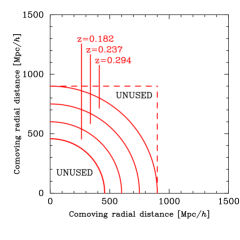
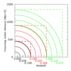
Figure 2: The configuration of spherical shells of projected matter density. The left panel illustrates how we place the outputs of the $N$-body simulations. There, the dashed line represents the original box size and each of the three shells is taken from the snapshot at different redshift. The right panel shows the nested structure of simulation boxes and the configuration of multiple lens shells. In the right panel, different colors are used to indicate different sets of simulations. The corresponding redshift of each shell is also shown at the bottom of the right panel.

We briefly summarize our ray-tracing simulations with full-sky coverage. The detailed description of our ray-tracing simulations is found in Appendix C. In our ray-tracing simulation, the light ray path and magnification matrix are calculated by the standard multiple lens-plane algorithm. The multiple lens-plane algorithm on a spherical geometry requires contiguous spherical shells of projected matter density. We thus utilize $N$-body simulations in Section 3.1 to generate a number of thin shells with width of $150\,h^{-1}$Mpc and produce three shells from a single simulation box as shown in the left panel of Figure 2. In order to extract a target shell region on a lightcone, we choose an appropriate snapshot at the redshift that correspond to the comoving distance to the shell from a hypothetical observer point (origin). A set of projected density shells are then configured using the nested structure of the simulation boxes. The right panel of Figure 2 shows the configuration of shells used in our ray-tracing simulations (only for $z\lower 2.15277pt\hbox{$\;\buildrel<\over{\sim}\;$}0.5$).

In this paper, we use HEALPix libraries for pixelization of a sphere (Górski et al., 2005). The angular resolution parameter $nside$ is set to be 4096. The corresponding angular resolution is $\simeq 0.86$ arcmin. For each shell, we calculate the projected mass density map from $N$-body particles using Nearest Grid Point method. Then, we perform the spherical harmonic transformation of the density shells to calculate the gravitational lensing potential on each shell via the Poisson equation (see, Eq. (105)). The obtained gravitational potential and its derivatives are used in the standard multiple lens-plane algorithm. In our simulation, we follow light ray trajectories from $z=0$ to $z=1$. The position of a ray and the magnification matrix $A_{ij}$ at each shell are updated by the recurrence relation as in e.g., Hilbert et al. (2009). The initial position of each ray is set to be the center of a pixel on HEALPix map. As a ray propagate with deflection, the position at each shell deviates from the position of the HEALPix map in general. We evaluate the potential at each shell by using an inverse-distant weighted interpolation of the potential field. The formalism of the multiple lens-plane method on a sphere is found in e.g., Teyssier et al. (2009); Becker (2013).

We obtain a total of ten all-sky convergence maps from ten sets of realization of $N$-body simulations. Note that we use different initial random seeds to generate $N$-body simulation data in order to avoid finding similar structures along a line of sight through ray-tracing. Figure 3 shows an example of our simulated convergence map on a full-sky.

3.3 Shape noise and sky mask

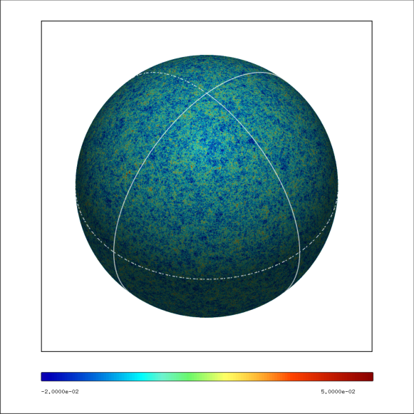
Figure 3: One of our simulated full-sky convergence maps. We perform the Gaussian smoothing with smoothing length of $2.12$ arcmin. The shape noise is not included in this figure. The red regions represent high convergence, while the blue regions correspond to negative convergence.

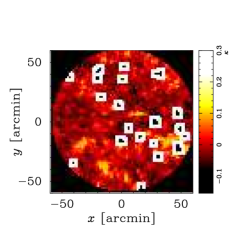
Figure 4: The configuration of the masked regions. In the left panel, black regions show the masks on the bright stars with the R-band magnitude of $M_{R}<10$. The right panel represents the typical configuration of the masks in a circular region with radius of 60 arcmin. Black isolated regions show masked regions due to the bright stars and white regions correspond to additional masked region. These white regions remove some pixels affected by the convolution of survey masks (black regions) with the smoothing filter.

We generate realistic mock catalogues by adding the effect of shape noise and sky mask to the obtained convergence maps. The intrinsic ellipticity of source galaxies is the main contaminant of cosmic shear measurement. We model the shape noise in a convergence map by assuming a two-dimensional Gaussian field as follows:

$$\langle\kappa_{\rm N}(\mbox{\boldmath$\theta$}_{i})\kappa_{\rm N}(\mbox{\boldmath$\theta$}_{j})\rangle=\frac{\sigma_{\gamma}^{2}}{2n_{\rm gal}\Omega_{\rm pix}}\delta_{ij},$$ (81)

where $\sigma_{\gamma}=0.4$, $n_{\rm gal}=10\,{\rm arcmin}^{-2}$, and $\Omega_{\rm pix}=4\pi/12/4096^{2}=6.24\times 10^{-8}\,{\rm str}$.

It is important to use a realistic sky mask to study statistics for upcoming lensing surveys. We here consider masks owing to bright stars. Among the planned HSC survey regions, we select two continuous regions with sky coverage of $\sim 565$ and $\sim 680$ squared degrees. J2000 coordinate of these regions are given by $22^{\rm h}00^{\rm m}<{\rm RA}<2^{\rm h}40^{\rm m},-1^{\circ}<{\rm DEC}<+7^{\circ}$ and $8^{\rm h}30^{\rm m}<{\rm RA}<15^{\rm h}00^{\rm m},-2^{\circ}<{\rm DEC}<+5^{\circ}$. In the following, we consider the bright stars with the R-band magnitude of $M_{R}<17$. We then select 1,149,871 stars located in these two regions from USNO-A2.0 catalog. In this paper, we assume the following relation between the R-band magnitude $M_{R}$ and the effective radius of a halo of bright star $r_{\rm star}$:

$$r_{\rm star}[{\rm arcsec}]=\left\{\begin{array}[]{ll}180&(M_{R}<9),\\ 0.2\times 10^{\left[13.75/M_{B}^{0.7}\right]}&(9\leq M_{R}\leq 17).\end{array}\right.$$ (84)

Then, we paste a circular mask with $r_{\rm star}$ around the pixel located at each star using Eq. (84). If $r_{\rm star}$ is less than the angular size of our all-sky map ($\sim$ 1 arcmin), we simply mask the pixel located in the star. After the above procedure, we further remove the “isolated” pixels whose surrounding pixels are all labeled as masked pixels. The final mask configuration generated in this way is shown in Figure 4. The left panel displays the masked region over the $565+680$ square degrees. The black dots shows the masked pixels on very bright stars $(M_{R}<10)$ and smaller masked regions are distributed in the white region homogeneously (but not shown in the figure). The mask covers over $\simeq 280$ squared degrees in total. The right panel shows an example of our masked sky simulation in a circular region with a radius of $1^{\circ}$.

From a single full-sky simulation, we make 20 mock HSC convergence maps with the masks by choosing the desired sky coverage ($565+680=1245$ squared degrees). We allow to have small overlap regions between the 20 masked maps. The overlap regions are located near the edge of the HSC sky coverage, and thus we expect this minor compromise does not affect the final results significantly. Finally, using 10 independent full-sky maps, we obtain a total of $20\times 10=200$ realizations of mock HSC lensing catalogs.

For a smoothed convergence map, we apply the different masking. As shown in Eq. (84), stars with $M_{R}>12$ have smaller mask radii than the pixel size in our simulation. Therefore, in principle, we can extract some information from the pixels where stars with $M_{R}>12$ are located. Because such faint stars would not affect the smoothed convergence map, we mask only the bright stars with the R-band magnitude of $M_{R}<12$. There are also ill-defined pixels that are compromised by the convolution with the smoothing filter. We remove such ill-defined pixels within 5 arcmin from the boundary of the mask regions. Consequently, masked regions on the smoothed convergence ${\cal K}$ maps differ from the original masked regions. Finally, we have a total of $\simeq 412$ squared degrees as unmasked regions. The corresponding sky fraction is $\sim$0.01.

4 RESULT

We present the weak lensing statistics measured from the full-sky simulations and also those from our 200 mock HSC catalogues. In the following, we define the threshold of lensing peak as ${\cal K}/\sigma_{\rm noise,0}$, where $\sigma_{\rm noise,0}$ is given by Eq. (12). Note that we use this definition also in the case without noise.

4.1 Ensemble average of statistics

All-sky

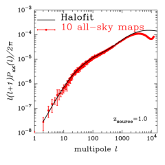
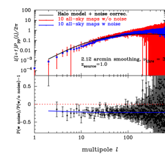
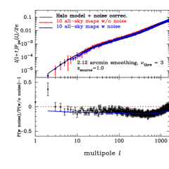
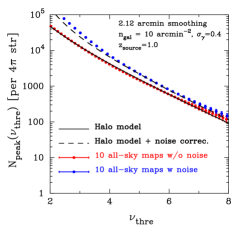
Figure 5: We compare the statistics measured from the ten all-sky simulations and our model prediction. In each panel, the black line is our halo model prediction. The red points with error bar represent the measured signal from the ’clean’ convergence maps without noise. The blue points show the result with noise. In the bottom portion in top right and the bottom left panel, we show the ratio of the two. The error bars indicate the standard deviation over ten realization. Note that the threshold of lensing peaks is defined by ${\cal K}/\sigma_{\rm noise,0}$ regardless of the presence or absence of noise.

We first show the ensemble average statistics over the ten full-sky simulations. They can be regarded as the expected values from an idealized full-sky observation. Figure 5 summarizes the measurements of $P_{\kappa\kappa},P_{{\rm p}{\rm p}},P_{{\rm p}\kappa}$ and $N_{\rm peak}$. We selected the lensing peaks with threshold of $\nu_{\rm thre}=3$ (or ${\cal K}\simeq 0.05$) in both the maps with and without shape noise. To calculate the correlation in harmonic space, we correct the pixelisation effect with the pixel window function of HEALPix. Overall, our model is in good agreement with the measurement from the full-sky simulations. In the case without shape noise, we calculate $P_{{\rm p}{\rm p}}$, $P_{{\rm p}\kappa}$ and $N_{\rm peak}$ assuming the one-to-one correspondence between lensing peaks and dark matter halos, i.e.,

$${\rm Prob}({\cal K}_{\rm peak,obs}|\,{\cal K}_{{\rm peak},h}(z,M))=\delta_{D}({\cal K}_{\rm peak,obs}-{\cal K}_{{\rm peak},h}(z,M)).$$ (85)

The results of $P_{{\rm p}{\rm p}}$ and $P_{{\rm p}\kappa}$ from the maps with and without noise show appreciable differences at large angular scales ($\ell\lower 2.15277pt\hbox{$\;\buildrel<\over{\sim}\;$}100$). This can be explained by the modulation of peak height due to the shape noise. When we select the lensing peaks with a given $\nu_{\rm thre}$, we effectively include less massive dark matter haloes as well in the noisy ${\cal K}$ maps. Then both $P_{{\rm p}{\rm p}}$ and $P_{{\rm p}\kappa}$ are reduced at large angular scales in the noisy maps because less massive halos have weaker clustering. Also, the number count of peaks in the noisy convergence maps is described well by our model as shown in Section 2.3. In the maps with shape noise, we detect more lensing peaks for a given threshold, for example, by a factor of $\sim 3$ for $\nu_{\rm thre}=3$.

Masked sky

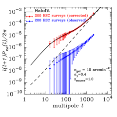
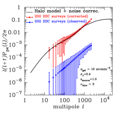
Figure 6: The auto- and cross-power spectra obtained from 200 mock HSC catalogues. The black line is the result of our halo model. In the left panel, the dashed line shows the shape noise contribution to convergence power spectrum.

In the presence of masks, we need the correction for the mode-coupling effects in measurements of power spectrum. We adopt the pseudo-spectrum estimator for this purpose (Hansen & Górski, 2003; Efstathiou, 2004; Brown, Castro & Taylor, 2005; Hikage et al., 2011). The basics of the method is summarized in Appendix D. In measurements of the binned two spectra $P_{\kappa\kappa}$ and $P_{{\rm p}\kappa}$, we follow the similar method shown in Brown, Castro & Taylor (2005); Hikage et al. (2011). Let us consider the $b$-th binned power spectrum in the multipole range of $\ell^{b}_{\rm min}<\ell<\ell^{b+1}_{\rm min}$. In this case, we can calculate the band-powers $(P_{b})$ as

$$P_{b}=\sum_{b^{\prime}}{\cal M}^{-1}_{bb^{\prime}}\sum_{\ell}{\cal B}_{b^{\prime}\ell}\tilde{P}(\ell),$$ (86)

where $\tilde{P}(\ell)$ is the measured power spectrum on a masked sky and ${\cal B}_{b\ell}$ is the binning operator, which is defined by

$${\cal B}_{b\ell}=\left\{\begin{array}[]{ll}\ell(\ell+1)/(2\pi)/(\ell^{b+1}_{\rm min}-\ell^{b}_{\rm min})&(\ell^{b}_{\rm min}<\ell<\ell^{b+1}_{\rm min}),\\ 0&({\rm otherwise}).\end{array}\right.$$ (89)

Here, we define the binned coupling matrix ${\cal M}_{bb^{\prime}}$ as

$${\cal M}_{bb^{\prime}}=\sum_{\ell}{\cal B}_{b\ell}M_{\ell\ell^{\prime}}Q_{\ell^{\prime}b^{\prime}},$$ (90)

where the definition of $M_{\ell\ell^{\prime}}$ is found in Appendix D and $Q_{b\ell}$ is given by

$$Q_{b\ell}=\left\{\begin{array}[]{ll}2\pi/[\ell(\ell+1)]&(\ell^{b}_{\rm min}<\ell<\ell^{b+1}_{\rm min}),\\ 0&({\rm otherwise}).\end{array}\right.$$ (93)

The number of bins is set to be 30. We perform the binning in linear spacing for the first 10 bins as $\ell^{b}_{\rm min}=2+10b\,(1\leq b\leq 10)$, while the remaining 20 bins have logarithmically equal spacing up to $\ell_{\rm max}=2000$. The measured and corrected binned power spectra are plotted in Figure 6. We use 200 masked sky simulations to calculate the average of the binned $P_{\kappa\kappa}$ and $P_{{\rm p}\kappa}$.

For cross-correlation, we find $\sim 100-200$ lensing peaks with $\nu_{\rm thre}=3$ on each simulated HSC map. In Figure 6, the blue points with error bars shows the measured spectrum, and the red points are the corrected spectrum with the pseudo-spectrum method. Clearly, we can recover the underlying power spectrum with the correction of the mode-coupling due to masks. The difference in amplitude can be explained approximately by the effective fraction of sky coverage $(\sim 0.01-0.02)$

4.2 Covariance

We use 200 masked sky simulations to calculate covariances between the weak lensing statistics of interest. First, we calculate the convergence power spectrum covariance. In the flat sky approximation and without masks, the covariance of the binned power spectrum is expressed as (e.g., Cooray & Hu, 2001)

$${\rm Cov}[P_{\kappa\kappa}(\ell_{i}),P_{\kappa\kappa}(\ell_{j})]=\frac{\delta_{ij}}{2\ell_{i}\Delta\ell f_{\rm sky}}2P_{\kappa\kappa}^{2}(\ell_{i})+\frac{1}{4\pi f_{\rm sky}}\int_{\ell_{i}}\,\frac{{\rm d}^{2}\mbox{\boldmath$\ell$}}{A_{s,i}}\int_{\ell_{j}}\,\frac{{\rm d}^{2}\mbox{\boldmath$\ell$}^{\prime}}{A_{s,j}}T_{\kappa\kappa\kappa\kappa}(\mbox{\boldmath$\ell$},-\mbox{\boldmath$\ell$},\mbox{\boldmath$\ell$}^{\prime},-\mbox{\boldmath$\ell$}^{\prime}),$$ (94)

where $P_{\kappa\kappa}(\ell_{i})$ represents the $i$-th binned power spectrum, $f_{\rm sky}$ is the fraction of sky covered by the observation, $\Delta\ell$ is the bin width in $\ell$ space, and $A_{s,i}$ is the area of the two-dimensional shell around the $i$-th bin $\ell_{i}$ in Fourier space. Here, $T_{\kappa\kappa\kappa\kappa}$ is the tri-spectrum of convergence, of which definition and modeling are found in Section 2.4. In practice, we simplify the second term in Eq. (94) as

$$\int_{\ell_{i}}\,\frac{{\rm d}^{2}\mbox{\boldmath$\ell$}}{A_{s,i}}\int_{\ell_{j}}\,\frac{{\rm d}^{2}\mbox{\boldmath$\ell$}^{\prime}}{A_{s,j}}T_{\kappa\kappa\kappa\kappa}(\mbox{\boldmath$\ell$},-\mbox{\boldmath$\ell$},\mbox{\boldmath$\ell$}^{\prime},-\mbox{\boldmath$\ell$}^{\prime})\rightarrow T_{\kappa\kappa\kappa\kappa}(\ell_{i},\ell_{i},\ell_{j},\ell_{j}).$$ (95)

In the presence of masked regions, the estimator of the binned power spectrum is given by more complex expressions given in Eq. (86). The mode-coupling due to masked regions induces the intricate correlation between different Fourier modes in the covariance of $P_{\kappa\kappa}$ (the exact expression is found in Appendix D). Nevertheless, in the case where the value of masked pixels is set to be either 0 or 1, we can use the simplified formula of covariances as shown in Efstathiou (2004). When we work with harmonic space, the approximated formula can be expressed as

$${\rm Cov}[P_{\kappa\kappa}(\ell_{1}),P_{\kappa\kappa}(\ell_{2})]_{\rm mask}\simeq\sum_{\ell^{\prime}_{1}\ell^{\prime}_{2}}\frac{1}{2\ell^{\prime}_{2}+1}(M^{\kappa\kappa})^{-1}_{\ell_{1}\ell^{\prime}_{1}}(M^{\kappa\kappa})^{-1}_{\ell_{2}\ell^{\prime}_{2}}M^{\kappa\kappa}_{\ell^{\prime}_{1}\ell^{\prime}_{2}}\left[2P_{\kappa\kappa}(\ell^{\prime}_{1})P_{\kappa\kappa}(\ell^{\prime}_{2})+\frac{1}{4\pi}\sqrt{(2\ell^{\prime}_{1}+1)(2\ell^{\prime}_{1}+2)}T_{\kappa\kappa\kappa\kappa}(\ell^{\prime}_{1},\ell^{\prime}_{1},\ell^{\prime}_{2},\ell^{\prime}_{2})\right],$$ (96)

where $M^{\kappa\kappa}_{\ell\ell^{\prime}}$ represents the mode-coupling matrix for convergence. In Eq. (96), we evaluate the term $T_{\kappa\kappa\kappa\kappa}$ by the tri-spectrum in harmonic space following Hu (2001) because we define $T_{\kappa\kappa\kappa\kappa}$ in the flat sky approximation.

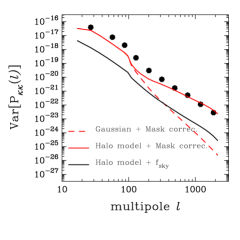
Figure 7: The variance of the psudo-spectrum estimator of $P_{\kappa\kappa}$ measured from 200 masked sky simulations. The black points show our measurement. The three lines represent the different contribution to variance. The black line is the simplest halo model with the sky fraction of $f_{\rm sky}=0.023$, while the red lines show the halo model covariance with the correction of the effect of masked regions. The red dashed line corresponds to the Gaussian model including the effect of masked region. For the red solid line, we take into account both non-Gaussianities caused by gravity and masked regions.

We can then examine the validity of Eq. (94) by using the measured covariance of $P_{\kappa\kappa}$ over 200 masked sky simulations. We use the same binning as in Section 4.1 but reduce the number of bins to 10 by taking average of the binned powers over nearest $\ell$ bins. Figure 7 shows the measured variance of the pseudo-spectrum estimator of $P_{\kappa\kappa}$. The black point shows the result obtained from the 200 simulations and the solid line represents our model of covariance in Eq. (94) with the appropriate value of $f_{\rm sky}$ for our simulations. Interestingly, although the simple model of Eq. (94) is expected to account for non-Gaussianities caused by gravity, it underestimates the actual covariance by a factor of $\sim 10$. The corrected covariance components are shown in Figure 7. The first term and second term in Eq. (96) are plotted as red dashed and red solid line, respectively. The overall amplitude of the variance can be explained by the mask correction, while the contribution from tri-spectrum dominates at $\ell\lower 2.15277pt\hbox{$\;\buildrel>\over{\sim}\;$}200$. Clearly, it is problematic to adopt the commonly used estimate of covariance given by in Eq. (94).

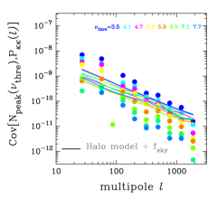
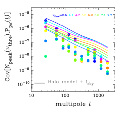
Figure 8: The cross covariance of weak lensing statistics calculated from the 200 simulations. In each panel, the black or colored points show the measured covariance, and the solid line shows the corresponding halo model prediction. We define the peaks with $\nu_{\rm thre}$ when measuring $P_{{\rm p}\kappa}$. In the bottom two panels, the color indicate the results for different threshold $\nu_{\rm thre}$ in $N_{\rm peak}$. The threshold value is varied in the range $\nu_{\rm thre}=3.5-7.7$.

To perform combined analysis of $P_{\kappa\kappa},P_{{\rm p}\kappa}$ and $N_{\rm peak}$, we need cross covariance between the statistics. Unfortunately, it is difficult to model the impact of masked region on the cross covariances in a similar manner to Eq. (96). Here, we simply compare the measured cross covariances with the prediction of our halo model. In the model, the covariance can be derived similarly to Eq. (94). For example,

$${\rm Cov}[P_{{\rm p}\kappa}(\ell_{i}),P_{{\rm p}\kappa}(\ell_{j})] = \frac{\delta_{ij}}{2\ell_{i}\Delta\ell f_{\rm sky}}\left(P_{{\rm p}{\rm p}}(\ell_{i})P_{\kappa\kappa}(\ell_{i})+P_{{\rm p}\kappa}(\ell_{i})P_{{\rm p}\kappa}(\ell_{i})\right)+\frac{1}{4\pi f_{\rm sky}}\int_{\ell_{i}}\,\frac{{\rm d}^{2}\mbox{\boldmath$\ell$}}{A_{s,i}}\int_{\ell_{j}}\,\frac{{\rm d}^{2}\mbox{\boldmath$\ell$}^{\prime}}{A_{s,j}}T_{{\rm p}\kappa{\rm p}\kappa}(\mbox{\boldmath$\ell$},-\mbox{\boldmath$\ell$},\mbox{\boldmath$\ell$}^{\prime},-\mbox{\boldmath$\ell$}^{\prime}),$$ (97)

$${\rm Cov}[P_{{\rm p}\kappa}(\ell_{i}),P_{\kappa\kappa}(\ell_{j})] = \frac{\delta_{ij}}{2\ell_{i}\Delta\ell f_{\rm sky}}2P_{{\rm p}\kappa}(\ell_{i})P_{\kappa\kappa}(\ell_{i})+\frac{1}{4\pi f_{\rm sky}}\int_{\ell_{i}}\,\frac{{\rm d}^{2}\mbox{\boldmath$\ell$}}{A_{s,i}}\int_{\ell_{j}}\,\frac{{\rm d}^{2}\mbox{\boldmath$\ell$}^{\prime}}{A_{s,j}}T_{{\rm p}\kappa\kappa\kappa}(\mbox{\boldmath$\ell$},-\mbox{\boldmath$\ell$},\mbox{\boldmath$\ell$}^{\prime},-\mbox{\boldmath$\ell$}^{\prime}),$$ (98)

where we have defined $T_{{\rm p}\kappa{\rm p}\kappa}$, $T_{{\rm p}\kappa\kappa\kappa}$, and the other covariances (i.e. ${\rm Cov}[N_{\rm peak},N_{\rm peak}]$, ${\rm Cov}[N_{\rm peak},P_{\kappa\kappa}]$, and ${\rm Cov}[N_{\rm peak},P_{{\rm p}\kappa}]$) in Section 2.4.

Figure 8 shows the measured peak-power cross-covariance. In constrast to the case of $P_{\kappa\kappa}$, the covariance including $P_{{\rm p}\kappa}$ and $N_{\rm peak}$ is less affected by masks: the simple model that accounts for $f_{\rm sky}$ yields a reasonable result with respect to that of the simulations. We find that the difference is by a factor of $\sim 3$ at most.

5 CONCLUSION AND DISCUSSION

We have performed all-sky lensing simulations to generate a large set of realistic weak lensing mass maps with complex masked regions by incorporating the actual position of bright stars. We have used the set of the mock samples to study the statistical properties of weak lensing convergence and convergence peaks in detail. Full nonlinear covariances between the statistics have been also calculated from 200 realization of masked maps. We have also developed an analytic halo model that provides reasonably accurate prediction for the statistics.

When adopting a Gaussian smoothing with the full width at half maximum of 5 arcmin, we can associate weak lensing convergence peaks with dark matter halos with mass of $\sim 10^{14}\,h^{-1}M_{\odot}$ at $z\sim 0.1-0.2$. We can also estimate the modulation of peak height due to shape noise by using a model based on Gaussian peak statistics. Thus, the abundance of peaks, the angular correlation function, and the cross-correlation of peaks and cosmic shear are all obtained accurately by our halo model approach with the shape noise correction. Furthermore, the halo model can also take the mask effect into account and indeed produces accurate ensemble average of statistics and their covariances. The impact of masked regions on the covariance can be described by the following two effects: (i) reduction of sky coverage and (ii) the mode-coupling effect between different Fourier modes. We find that the former affects the overall amplitude of cross-covariance between statistics, while the latter is important for the covariance of cosmic shear power spectrum $P_{\kappa\kappa}$. For the masked regions adopted here, ignoring the mode-coupling effect would induce underestimation of the covariance of $P_{\kappa\kappa}$ by a factor of $\sim 10$(!).

The number density of source galaxies is an important factor in the statistical analysis of weak gravitational lensing. As one may expect, a large number density of sources is desired to find clusters with high accuracy and perform cosmological analysis with selected clusters. In comparison with the case of $n_{\rm gal}=10\,{\rm arcmin}^{-2}$, we have confirmed that the signal-to-noise ratio increase by a factor of $\sim 1.5$ in combined analysis with $P_{\kappa\kappa}$, $P_{{\rm p}\kappa}$ and $N_{\rm peak}$ even if we ignore the shape noise contaminant (i.e., $n_{\rm gal}\rightarrow\infty$). This suggests that imaging over a wide area is suitable for cosmological analysis with the lensing statistics even if the number density of sources is not significantly increased in such surveys.

We have also examined the validity of our model for two additional cases: $n_{\rm gal}=5$ and 30 ${\rm arcmin}^{-2}$. When the smoothing scale, the rms of intrinsic ellipticity, and the source redshift are all fixed, the halo model prediction is in good agreement with the result of our full-sky simulations in the case of $n_{\rm gal}=30\,{\rm arcmin}^{-2}$, but the agreement is worse with $n_{\rm gal}=5\,{\rm arcmin}^{-2}$ . Therefore, when we consider the typical value of the rms of intrinsic ellipticity and the source redshift, our model is expected to be accurate when $n_{\rm gal}\lower 2.15277pt\hbox{$\;\buildrel>\over{\sim}\;$}10\,{\rm arcmin}^{-2}$ with $\sim 2$ arcmin Gaussian smoothing.

Our model has been successfully applied the statistics of a smoothed convergence map with shape noise. In principle, one can find an optimal filter function so that the number of detected clusters is increased (e.g. Hennawi & Spergel, 2005; Maturi et al., 2005). Our model is based on the assumption that shape noise in a smoothed lensing map has Gaussian properties. The assumption is valid when the ellipticities of the source galaxies are uncorrelated and when there are a sufficient number of source galaxies per pixel (i.e. the central limit theorem). We expect that, while our model can be applied to the general form of filter function, it may not be appropriate when there are only few source galaxies and/or when there is no one-to-one correspondence between peaks and halos.

Clusters of galaxies are important targets in future cosmological surveys. Selecting galaxy clusters based on cosmic shear measurement does not rely on mass estimate nor on calibration with additional information such as $X$-ray brightness. Nevertheless, there remain some systematic effects worth mentioning here.

Gravitational lensing causes not only distortion of source images but also magnification. Using magnified galaxies in a flux- and size-limited survey would potentially cause systematic effect(s) in the weak lensing statistics. The magnification effects on lensing peak statistics have been already studied in e.g., Schmidt & Rozo (2011). Recent numerical study by Liu et al. (2014a) suggests that the magnification effect causes non-negligible bias in parameter estimation in the case of LSST. In order to examine the magnification effect further, it is essential to run high angular resolution simulations. This is because the mean number of source galaxies on each pixel should be less than unity to make the one-to-one correspondence between a pixel and a (magnified) source galaxy. In the case of $n_{\rm gal}=10\,{\rm arcmin}^{-2}$, we should set the pixel size to be $1/\sqrt{n_{\rm gal}}\sim 0.3\,{\rm arcmin}$. We will perform such simulations to study the magnification effect in wide-field surveys in detail.

Another important issues are uncertainties and systematic bias associated with baryonic effects. Previous studies (e.g., Semboloni et al., 2011; Semboloni, Hoekstra & Schaye, 2013; Zentner et al., 2013) explored the impact of the baryonic component to two-point statistics of cosmic shear and consequently to cosmological parameter estimation. The baryonic effect is likely important in weak lensing peak statistics. Indeed, Yang et al. (2013) show appreciable baryonic effects on peak statistics using a simple model applied to dark-matter-only simulations, whereas the baryonic effect on higher order convergence statistics have been studied with numerical simulations (Osato, Shirasaki & Yoshida, 2015). Recently, Mohammed et al. (2014) explored halo model approach to include the baryonic effect on cosmic shear statistics.

The statistical properties and the intrinsic correlation of source galaxies and lensing structures are still uncertain but could be critical when making a large lensing mass maps. Among such correlations, source-lens clustering (e.g., Hamana et al., 2002) and the intrinsic alignment (e.g., Hirata & Seljak, 2004) are likely to compromise cosmological parameter estimation. A promising approach in theoretical studies would be associating the source positions with their host dark matter halos on the light cone. This is along the line of our ongoing study using a large set of cosmological simulations.

Weak gravitational lensing is a promising tool to probe the dark matter distribution in the universe. Statistical analysis of a reconstructed mass map can be performed to extract precise cosmological information. The peak statistics considered in the present paper contain the information related to massive objects such as clusters of galaxies and thus have a great potential to probe cosmology and constrain the model of structure formation simultaneously. Ongoing/upcoming imaging surveys such as HSC, DES, and LSST in the near future, will provide the largest dark matter map we have never seen before. We expect our study presented here provides a useful guide to interprete properly the reconstructed mass map and to reveal the nature of the dark components in the universe.

Appendix A HALO-PEAK MATCHING

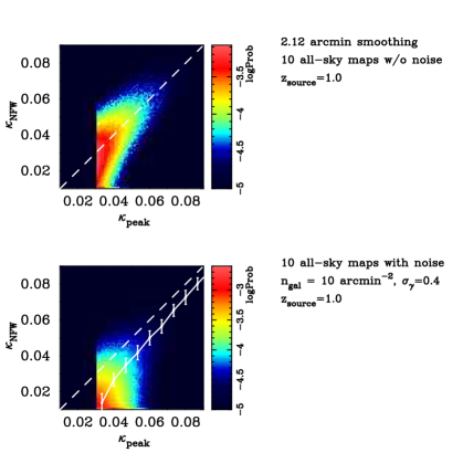
Figure 9: The correspondence between dark matter halos and lensing peaks. The top panel shows the scatter plot of peak height and the expected convergence by the matched halos in absence of noise. The lower panel corresponds to the case with shape noise. In each panel, the horizontal axis represents the peak height and the vertical axis shows the expected convergence of NFW halos.

In this appendix, we examine the correspondence between dark matter halos and the local maximum in lensing convergence map.

In order to generate mock halo catalogs, we identify dark matter halos in outputs of our $N$-body simulation (see, Section 3.1) using the standard friends-of-friends algorithm with a linking parameter of $b=0.2$ in units of the mean particle separation. We use dark matter halos with mass greater than $10^{13}\,h^{-1}M_{\odot}$ in the following analysis. This lowest mass corresponds to the mass of $20$ particles in the largest simulation. Then, the position of dark matter halo in $N$-body simulations are arranged in the same way as in the ray-tracing experiments in Section 3.2.

With our ray-tracing simulations and mock halo catalogs, we study the correspondence between halos and the peaks in weak lensing convergence maps. We first identify the local maxima in the smoothed lensing convergence field with source redshift of $z_{\rm source}=1$. In this appendix, we again adopt the Gaussian smoothing with the full width at half maximum of 5 arcmin. When including the shape noise in convergence maps, we set $\sigma_{\gamma}=0.4$ and $n_{\rm gal}=10\,{\rm arcmin}^{-2}$. For selection of peaks, the threshold of peak height is set to be ${\cal K}=0.03$. This value corresponds to $\sim 3\sigma$ in smoothed convergence maps without noise. For a given position of lensing peak, we search for the matched dark matter halos within a radius of 5 arcmin from the peak position. This search radius is set to be larger than the smoothing scale but still smaller than the angular size of massive halos at $z\sim 0.1-0.2$ (also see, Hamana, Takada & Yoshida, 2004). When we find several halos in search radius, we regard the matched halo as the closest halo from the position of peak. For each matched peak, we estimate the corresponding convergence by using the universal NFW density profile (see Section 2.2 in detail). In the calculation of expected convergence from FoF halos, we simply assume that the FoF mass is equal to the virial mass. In total, we find 632,238 and 1,404,538 pairs of peaks and halos over 10 noise-less maps and noisy maps, respectively.

Figure 9 shows the scatter plot of peak height in ${\cal K}$ map and the expected convergence by NFW halos. The horizontal axis corresponds to peak height, while the vertical axis shows the corresponding convergence expected by NFW halos. Thus, the color map in each panel shows the probability of Eq. (23). We present the line of $y=x$ as the dashed line in each panel. In lower panel of this figure, we show the effect of the modulation of peak height as the solid line with error bars. The solid line is derived by ${\bar{\cal K}}_{\rm peak,obs}(z,M)$ in Eq. (28) and the error bars reflect the scatter of ${\bar{\cal K}}_{\rm peak,obs}(z,M)$. As shown in previous works, we confirm the good correspondence between the matched dark matter halos and lensing peaks in the noise-less maps. Also, our model as shown in Eq. (28) can explain the average relation between peaks and dark matter halos even in the case with noise.

Appendix B THE CASE OF COMPENSATED GAUSSIAN FILTER

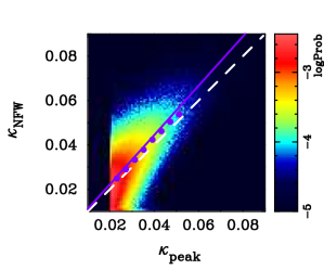
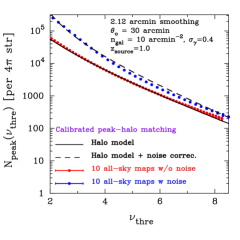
Figure 10: The property of lensing peaks on smoothed maps by the compensated Gaussian filter. The left panel shows the scatter plot of peak height and the expected convergence by the matched halos in absence of noise. In the left panel, the dashed line shows one-to-one correspondence. The purple points represent the mean relation of the expected convergence and measured peak height and the best-fit linear relation is expressed as the purple line. The right panel shows the comparison the peak abundance measured from ten full-sky simulations and our model prediction. In the right panel, the black line is our halo model prediction. The red points with error bar represent the measured signal from the ’clean’ convergence maps without noise. The blue points show the result with noise. We normalize the measured peak height by $\sigma_{\rm noise,0}$ in both cases with and without noise. The error bars indicate the standard deviation over ten realization. In the calculation of peak count, we correct the biased relation of $\kappa_{\rm NFW}$ and $\kappa_{\rm peak}$ as shown in the purple line in the left panel. The details of correction are found in the text.

We examine another practical filter function to construct smoothed lensing maps. In this appendix, we consider $z_{\rm source}=1$, and we set $\sigma_{\gamma}=0.4$ and $n_{\rm gal}=10\,{\rm arcmin}^{-2}$ when including the shape noise in convergence maps.

We first consider the compensated filter $U_{\rm c}$ based on the Gaussian form as

$$U_{\rm c}(\theta)=\frac{1}{\pi\theta_{G}^{2}}\exp\left(-\frac{\theta^{2}}{\theta_{G}^{2}}\right)-\frac{1}{\pi\theta_{o}^{2}}\left[1-\exp\left(-\frac{\theta_{o}^{2}}{\theta_{G}^{2}}\right)\right],$$ (99)

where $\theta_{o}$ represents the boundary of the filter and we set $U_{\rm c}$ to be zero for $\theta>\theta_{o}$. We adopt the smoothing scale of $\theta_{G}=5/\sqrt{8\ln 2}$ arcmin and $\theta_{o}=30$ arcmin. For the compensated filter function of $U_{\rm c}$, the noise power spectrum on a smoothed lensing map is expressed as (van Waerbeke, 2000)

$$P_{\cal N}(\ell)=\frac{\sigma_{\gamma}^{2}}{2n_{\rm gal}}|{\tilde{U}}_{\rm c}(\ell)|^{2},$$ (100)

where $\sigma_{\gamma}$ is the rms of the intrinsic ellipticity of sources, $n_{\rm gal}$ represents the number density of source galaxies, and ${\tilde{U}}_{\rm c}$ is the Fourier transform of $U_{\rm c}$. As shown in Eq. (12), the noise variance $\sigma_{\rm noise,0}$ is evaluated by the integral of $P_{\cal N}(\ell)$ in Fourier space. In the case of $\theta_{o}=30$ arcmin, the boundary of the filter changes $\sigma_{\rm noise,0}$ by about 1% compared to the case of the usual Gaussian filter. Thus, we can safely ignore the difference of $\sigma_{\rm noise,0}$ between the compensated and the usual Gaussian filter for our parameter choice.

In order to investigate the effect of the modification of filter function on lensing peak statistics, we first study the correspondence between peaks and halos by the halo-peak matching analysis as shown in Appendix A. When we limit lensing peaks with the height larger than $0.02$, we find 1,045,291 matched pairs over ten full-sky maps without shape noise. The left panel in figure 10 shows the scatter plot of the measured peak height and the expected convergence signal for the spherical NFW halo. In the calculation of expected signal, we simply assume that FoF mass of halos is equal to the virial mass and use the model of concentration parameter $c_{\rm vir}$ in Duffy et al. (2010). We expect that the one-to-one correspondence between peaks and halos would still hold. However, we find biased relation between the mean measured height and expected one even in the absence of noise. The biased mean relation is shown by the purple points in the left panel in figure 10. It can also be fitted well by linear relation of ${\cal K}_{\rm peak}=\alpha{\cal K}_{\rm NFW}+\beta$. We find the best-fit value of $\alpha$ is 0.9 while the offset $\beta$ can be approximated to be zero. A similar relation is also found by Hamana et al. (2012). It might be caused as a consequence of various effects such as the mismatch of FoF mass and virial mass defined by spherical over-density.

Even without knowing the origin of the biased relation, we can still predict the lensing peak statistics with the compensated filter by adopting the biased relation in our halo model. Our approach is simply to replace ${\cal K}_{{\rm peak},h}(z,M)$ with $\alpha{\cal K}_{{\rm peak},h}(z,M)+\beta$ for the calculation of Eq. (23). Here, we also assume that ${\cal K}_{{\rm peak},h}$ can be evaluated by

$${\cal K}_{{\rm peak},h}(z,M)=\int{\rm d}^{2}\theta\,U_{\rm c}(\theta;\theta_{G},\theta_{o})\kappa_{h}(\theta|z,M),$$ (101)

where $\kappa_{h}(\theta|z,M)$ represents the convergence profile of spherical NFW halos with mass of $M$ and the redshift of $z$. With the above correction, our model can provide a reasonable fit to the measured peak statistics from ten full-sky maps as shown in the right panel in figure 10. The right panel shows the measured peak count for the compensated filter with and without shape noise. In the right panel, the black solid (dashed) line represent our halo model in absence (presence) of noise with the correction for the biased relation of ${\cal K}_{\rm peak}$ and ${\cal K}_{\rm NFW}$. With the above suitable modifications, our model works as long as the one-to-one correspondence of peaks and halos holds. We simply need to calibrate the mean scaling relation of ${\cal K}_{\rm peak,obs}$ and ${\cal K}_{{\rm peak},h}$ in absence of noise.

Appendix C FULL SKY RAY-TRACING SIMULATION

Here we first summarize basic equations of the multiple-plane gravitational lensing algorithm, and then describe the ray-tracing method through the multiple-plane. For the former we largely follow Das & Bode (2008), and for the latter we adopt one developed by Teyssier et al. (2009).

Throughout this section, we work on the comoving coordinates. Thus $\rho$, $\chi$, and $r(\chi)$ denote the comoving matter density, the radial comoving distance, and the comoving angular diameter distance, respectively.

C.1 Construction of the lensing potentials of multiple-plane

The 3-dimensional light-cone matter distribution is composed of the multiple-layer of shells with a fixed width of $150\,h^{-1}$Mpc taken from the nested simulation boxes. The surface matter density field on a sphere for $j$-th shell is defined by

$$\Delta_{\Sigma}^{j}(\mbox{\boldmath$\theta$})=\int_{\rm shell}{\rm d}\chi~{}(\rho(\mbox{\boldmath$\theta$},\chi)-\bar{\rho})r(\chi)^{2},$$ (102)

where $\theta$ denote the angular directions and $\bar{\rho}$ corresponds the mean matter density, and the integration is over the shell width. We set the lens-planes for each shell at the cone-volume weighted mean distance, $\chi_{j}=0.75(\chi_{j,\rm max}^{4}-\chi_{j,\rm min}^{4})/(\chi_{j,\rm max}^{3}-\chi_{j,\rm min}^{3})$, where $\chi_{j,\rm max}$ and $\chi_{j,\rm min}$ are the farthest and nearest radial distance to a shell, respectively. The convergence field for $j$-th shell is given by

$$K^{j}(\mbox{\boldmath$\theta$})={{4\pi G}\over c^{2}}{{\Delta_{\Sigma}^{j}(\mbox{\boldmath$\theta$})}\over{a_{j}r(\chi_{j})}}$$ (103)

where $a_{j}$ is the scale factor at the lens-plane $\chi_{j}$. We use the HEALPix (Górski et al., 2005) scheme for pixelization of a sphere, and we make the best use of the HEALPix library. For each shell, we construct the projected mass density map from $N$-body particles using Nearest Grid Point method (implemented with HEALPix subroutine vec2pix_ring). Using the volume ($V_{\rm sim}$) and total number of $N$-body particles ($N_{\rm part}$) of the $N$-body simulations, the total number of pixels ($npix$), the number of $N$-body particles within $i$-th pixel ($n_{{\rm pix},i}$) and its mean value ($\bar{n}_{\rm pix}$), the convergence field is given by

$$K^{j}(\mbox{\boldmath$\theta$}_{i})={{3\Omega_{m}}\over{2a_{j}r(\chi_{j})}}\left({{H_{0}}\over c}\right)^{2}{{V_{\rm sim}}\over{N_{\rm part}}}{{npix}\over{4\pi}}(n_{{\rm pix},i}-\bar{n}_{\rm pix}).$$ (104)

Having the convergence field being ready, we expand it in spherical harmonics to have its coefficients, $K_{lm}^{j}$, using the HEALPix subroutine map2alm. Then, the spherical harmonics coefficients for the lensing potential $\phi^{j}$ can be obtained via

$$\phi_{lm}^{j}={2\over{l(l+1)}}K_{lm}^{j}\mbox{~{}~{} for $l\neq 0$,}$$ (105)

and $\phi_{lm}^{j}=0$ for $l=0$. This gives us the lensing potential field on a sphere, and its 1st and 2nd derivatives relate to the gravitational lensing deflection field ($\alpha_{i}^{j}=-\nabla_{\hat{n}_{i}}\phi^{j}$) and the optical tidal matrix ($U_{ik}^{j}=-\nabla_{\hat{n}_{i}}\nabla_{\hat{n}_{j}}\phi^{j}$), respectively. Note that $\nabla_{\hat{n}_{i}}$ ($i=1,2$) denotes the angular derivative. In an actual computation, we utilize the HEALPix subroutine alm2map_der.

C.2 Light ray propagation

Let us first describe the method to trace the ray trajectory using the multiple-plane algorithm, for which we basically follow one developed by Teyssier et al. (2009). A virtual observer is located at the center of the nested simulation boxes. Rays are traced backward from the observer point with the initial ray directions being set on HEALPix pixel centers. Thus the ray positions on the 1st (closest to the observer) is exactly at the HEALPix pixel centers. At each lens-plane, the ray directions are deflected according to $\alpha_{i}^{j}$, and the ray positions on the next lens-plane are computed using the method described in Appendix A of Teyssier et al. (2009). Note that ray positions on the $j$-th ($j>1$) lens-plane are not exactly at the pixel center due to the lensing deflections, however the lensing fields ($\alpha_{i}^{j}$, $U_{ik}^{j}$) are only computed at the pixel centers. In order to evaluate the lensing fields at an arbitrary position ($\theta$), we adopt the inverse distance weighted interpolation from nearest four pixel values;

$$\alpha_{i}^{j}(\mbox{\boldmath$\theta$})={{\sum_{k=1}^{4}w_{k}\alpha_{i}^{j}(\mbox{\boldmath$\theta$}_{k}\rightarrow\mbox{\boldmath$\theta$})}\over{{\sum_{k=1}^{4}w_{k}}}},$$ (106)

where $w_{k}=1/|\mbox{\boldmath$\theta$}-\mbox{\boldmath$\theta$}_{k}|$, and $\alpha_{i}^{j}(\mbox{\boldmath$\theta$}_{k}\rightarrow\mbox{\boldmath$\theta$})$ is the deflection angle at the pixel center $\mbox{\boldmath$\theta$}_{k}$ but after parallel transporting to the ray position $\theta$ (in order to take into account the change in the local ($\mbox{\boldmath$e$}_{\theta},\mbox{\boldmath$e$}_{\phi}$) basis). In the actual computation, the parallel transport of the vector and tensor (for $U_{ik}^{j}$ described below) is implemented by the rotation of them by an angle between two coordinate bases at $\mbox{\boldmath$\theta$}_{k}$ and $\theta$ (see Appendix C of Becker, 2013).

Having evaluated the ray positions at a lens-plane, we are able to compute the lensing magnification matrix ($A_{ik}^{j}$) using the recurrence relation (Hilbert et al., 2009; Becker, 2013);

$$A_{ik}^{j+1} = \left(1-{{r(\chi_{j})}\over{r(\chi_{j+1})}}{{r(\chi_{j+1}-\chi_{j-1})}\over{r(\chi_{j}-\chi_{j-1})}}\right)A_{ik}^{j-1}+{{r(\chi_{j})}\over{r(\chi_{j+1})}}{{r(\chi_{j+1}-\chi_{j-1})}\over{r(\chi_{j}-\chi_{j-1})}}A_{ik}^{j}-{{r(\chi_{j+1}-\chi_{j})}\over{r(\chi_{j-1})}}U_{im}^{j}A_{mk}^{j},$$

$$A_{ik}^{1} = \delta_{ik},$$ (107)

$$A_{ik}^{0} = \delta_{ik},$$

for $j\geq 1$, and note that in our notation, the lens-plane closest to the observer is $j=1$. The optical tidal matrix, $U_{ik}^{j}$, in the above relation is evaluated at the ray position on each lens-plane in the same interpolation scheme as eq. (106), and then again parallel transporting to the unperturbed ray position (i.e., the initial ray direction), because the observed magnification matrix should be evaluated in the local basis of the image position.

We choose the source-plane at an arbitrary redshift $z_{s}$ (and thus the correspondence radial distance to the source-plane $\chi_{s}$), and evaluate the source position on the source-plane and the magnification matrix by using the above methods but replacing, e.g., $\chi_{j+1}\rightarrow\chi_{s}$.

C.3 Image positions of haloes

The 3-dimensional light-cone distribution of dark matter haloes is generated in the same manner as for the matter distribution. The spatial position of a halo is converted into the angular position $\mbox{\boldmath$\theta$}_{S}^{\rm halo}$, where the subscript “_S” means the source position. We search for the corresponding image position $\mbox{\boldmath$\theta$}_{I}^{\rm halo}$ in the following manner. First, we search for the nearest ray to the halo source position on the lens-plane of the shell where the halo is located. The displacement vector between the angular positions of the halo and the nearest ray is computed, $\mbox{\boldmath$\Delta\theta_{S}$}=\mbox{\boldmath$\theta$}_{S}^{\rm halo}-\mbox{\boldmath$\theta$}_{S}^{\rm ray}$. This vector is parallel transported to the image position of the nearest ray $\mbox{\boldmath$\theta$}_{I}^{\rm ray}$, and we denotes it by $\Delta\theta_{I}$ Then the image position of the halo is given by $\mbox{\boldmath$\theta$}_{I}^{\rm halo}=\mbox{\boldmath$\theta$}_{I}^{\rm ray}+\mbox{\boldmath$\Delta\theta_{I}$}$. The last step is valid if the difference in the lensing deflection angles between ray-trajectory to the halo and the nearest ray is very small. The statistical properties of differences in the lensing deflection angles between nearby two rays (the, so-called, the lensing excursion angle) were studies in Hamana & Mellier (2001); Hamana et al. (2005). They found that the root-mean-square (rms) value of the lensing excursion angles of rays for $z_{s}=1$ with the separation of 1 arcmin is $\sim 1$ arcsec. This value can be considered as the typical error in $\mbox{\boldmath$\theta$}_{I}^{\rm halo}$. Considering the fact that the pixel scale of the current ray-tracing simulation is $\sim 1$ arcmin, we may conclude that the above approximation is reasonably valid. However it should be noticed that for rays gone through a strong lensing region, the excursion angle can be much larger than the rms value, and thus $\mbox{\boldmath$\theta$}_{I}^{\rm halo}$ may not be very accurate. There is room for improvement on this issue that we leave for future work.

Appendix D STATISTICAL PROPERTY OF PSEUDO-SPECTRUM ESTIMATORS

In this appendix, we summarize the statistical property of pseudo-spectrum estimators. The pseudo-spectrum method is a powerful framework to construct the power spectrum of an underlying random field on limited sky (e.g., Hansen & Górski, 2003; Efstathiou, 2004; Brown, Castro & Taylor, 2005).

Let us consider the two random fields in each direction in the sky: convergence field $\kappa(\Omega)$ and number density field of lensing peaks $p(\Omega)$. These two fields would commonly be expanded in spherical harmonic as follows:

$$\kappa(\Omega)=\sum_{\ell m}\kappa_{\ell m}{\cal Y}_{\ell m}(\Omega),$$ (108)

where ${\cal Y}_{\ell m}(\Omega)$ represents the spherical harmonics and we can define $p_{\ell m}$ for the random field $p(\Omega)$ similarly. The inverse transform is then given by

$$\kappa_{\ell m}=\int{\rm d}\Omega\,\kappa(\Omega){\cal Y}_{\ell m}(\Omega),$$ (109)

and the similar relation can be adopted for $p_{\ell m}$.

The effect of finite sky coverage for each field is characterized as

$$\tilde{\kappa}(\Omega) = W^{\kappa}(\Omega)\kappa(\Omega),$$ (110)

$$\tilde{p}(\Omega) = W^{p}(\Omega)p(\Omega),$$ (111)

where $W^{\kappa}$ and $W^{p}$ are the window function of sky masking for $\kappa$ and $p$, respectively. Thus, the harmonic modes in presence of masked region is expressed as

$$\tilde{X}_{\ell m}=\sum_{\ell^{\prime}m^{\prime}}W^{X}_{\ell m\ell^{\prime}m^{\prime}}X_{\ell^{\prime}m^{\prime}},$$ (112)

where $X=\kappa$, $p$ and $W^{X}_{\ell m\ell^{\prime}m^{\prime}}$ is defined by

$$W^{X}_{\ell m\ell^{\prime}m^{\prime}}=\int{\rm d}\Omega\,{\cal Y}_{\ell^{\prime}m^{\prime}}(\Omega)W^{X}(\Omega){\cal Y}^{*}_{\ell m}(\Omega).$$ (113)

The estimators of power spectra on limited sky is defined by

$$\tilde{\mbox{\boldmath$P$}}(\ell)=\frac{1}{2\ell+1}\sum_{m}\langle\tilde{\mbox{\boldmath$X$}}_{\ell m}\tilde{\mbox{\boldmath$X$}}_{\ell m}^{\dagger}\rangle,$$ (114)

where $\tilde{\mbox{\boldmath$X$}}_{\ell m}=(\tilde{\kappa}_{\ell m},\tilde{p}_{\ell m})$ and $\langle\tilde{\mbox{\boldmath$X$}}_{\ell m}\tilde{\mbox{\boldmath$X$}}_{\ell m}^{\dagger}\rangle$ represents the following set of power spectra:

$$\langle\tilde{\mbox{\boldmath$X$}}_{\ell m}\tilde{\mbox{\boldmath$X$}}_{\ell m}^{\dagger}\rangle=\left(\begin{array}[]{cc}\langle\tilde{\kappa}_{\ell m}\tilde{\kappa}^{*}_{\ell m}\rangle&\langle\tilde{\kappa}_{\ell m}\tilde{p}^{*}_{\ell m}\rangle\\ \langle\tilde{p}_{\ell m}\tilde{\kappa}^{*}_{\ell m}\rangle&\langle\tilde{p}_{\ell m}\tilde{p}^{*}_{\ell m}\rangle\\ \end{array}\right).$$ (117)

For the underlying field $\mbox{\boldmath$X$}=(\kappa,p)$, we can define the power spectra $\mbox{\boldmath$P$}(\ell)$ as

$$\mbox{\boldmath$P$}(\ell)=\langle\mbox{\boldmath$X$}_{\ell m}\mbox{\boldmath$X$}_{\ell^{\prime}m^{\prime}}^{\dagger}\rangle\delta_{\ell\ell^{\prime}}\delta_{mm^{\prime}}.$$ (118)

Using Eqs. (113) and (118), we can find the relation between $\tilde{\mbox{\boldmath$P$}}(\ell)$ and ${\mbox{\boldmath$P$}}(\ell)$ as follows:

$$\tilde{\mbox{\boldmath$P$}}(\ell) = \frac{1}{2\ell+1}\sum_{m}\sum_{\ell^{\prime}m^{\prime}}\mbox{\boldmath$W$}_{\ell m\ell^{\prime}m^{\prime}}\mbox{\boldmath$P$}(\ell^{\prime})(\mbox{\boldmath$W$}_{\ell m\ell^{\prime}m^{\prime}})^{\dagger},$$ (119)

$$= \sum_{\ell^{\prime}}\mbox{\boldmath$M$}_{\ell\ell^{\prime}}\mbox{\boldmath$P$}(\ell^{\prime}),$$ (120)

where $\mbox{\boldmath$W$}_{\ell m\ell^{\prime}m^{\prime}}$ is defined by

$$\mbox{\boldmath$W$}_{\ell m\ell^{\prime}m^{\prime}}=\left(\begin{array}[]{cc}W^{\kappa}_{\ell m\ell^{\prime}m^{\prime}}&0\\ 0&W^{p}_{\ell m\ell^{\prime}m^{\prime}}\\ \end{array}\right).$$ (123)

The matrix $\mbox{\boldmath$M$}_{\ell\ell^{\prime}}$ represents the mode coupling effect due to masked region on power spectra, which is given by (in terms of $\mbox{\boldmath$P$}(\ell)=(P_{\kappa\kappa}(\ell),P_{{\rm p}\kappa}(\ell),P_{{\rm pp}}(\ell))^{T}$),

$$\mbox{\boldmath$M$}_{\ell\ell^{\prime}}=\left(\begin{array}[]{ccc}M^{\kappa\kappa}_{\ell\ell^{\prime}}&0&0\\ 0&M^{p\kappa}_{\ell\ell^{\prime}}&0\\ 0&0&M^{pp}_{\ell\ell^{\prime}}\\ \end{array}\right),$$ (127)

where

$$M^{XY}_{\ell\ell^{\prime}} = \sum_{mm^{\prime}}W^{X}_{\ell m\ell^{\prime}m^{\prime}}\left[W^{Y}_{\ell m\ell^{\prime}m^{\prime}}\right]^{*},$$ (128)

$$= \frac{2\ell^{\prime}+1}{4\pi}\sum_{L}{\cal W}^{XY}_{L}\left(\begin{array}[]{ccc}\ell&\ell^{\prime}&L\\ 0&0&0\\ \end{array}\right)^{2},$$ (131)

and ${\cal W}^{XY}_{\ell}$ is given by

$${\cal W}^{XY}_{\ell} = \sum_{m}w^{X}_{\ell m}\left(w^{Y}_{\ell m}\right)^{*},$$ (132)

$$w^{X}_{\ell m} = \int{\rm d}\Omega\,W^{X}(\Omega){\cal Y}_{\ell m}(\Omega).$$ (133)

Hence, we can construct the estimator of $\mbox{\boldmath$P$}(\ell)$ from $\tilde{\mbox{\boldmath$P$}}(\ell)$ as

$$\hat{\mbox{\boldmath$P$}}(\ell)=\sum_{\ell^{\prime}}\mbox{\boldmath$M$}^{-1}_{\ell\ell^{\prime}}\tilde{\mbox{\boldmath$P$}}(\ell^{\prime}),$$ (134)

where $\hat{\mbox{\boldmath$P$}}(\ell)$ is so-called psuedo-spectrum estimators.

Next, we consider the covariance of the pseudo-spectrum estimators. The covariance of $\hat{\mbox{\boldmath$P$}}(\ell)$ is defined by

$${\rm Cov}[\hat{P}_{XY}(\ell),\hat{P}_{MN}(\ell^{\prime})]=\langle\hat{P}_{XY}(\ell)\hat{P}_{MN}(\ell^{\prime})\rangle-\langle\hat{P}_{XY}(\ell)\rangle\langle\hat{P}_{MN}(\ell)\rangle,$$ (135)

where $X,Y,M,N$ is set to be $\kappa$ or $p$. When the underlying field follows non-Gaussian and there exist no masked regions, the covariance can be expressed as

$${\rm Cov}[P_{XY}(\ell),P_{MN}(\ell^{\prime})]_{\rm all-sky}=\frac{\delta_{\ell\ell^{\prime}}}{2\ell+1}\left[P_{XM}(\ell)P_{YN}(\ell^{\prime})+P_{XN}(\ell)P_{YM}(\ell^{\prime})\right]+\frac{1}{2\ell+1}\frac{1}{2\ell^{\prime}+1}\sum_{mm^{\prime}}\langle X_{\ell m}Y^{*}_{\ell m}M_{\ell^{\prime}m^{\prime}}N^{*}_{\ell^{\prime}m^{\prime}}\rangle_{c},$$ (136)

where the first term of the right-hand side in Eq. (136) represents the Gaussian contribution to the covariance matrix and the second term corresponds to the contribution of four-point correlation function due to non-Gaussianity in the underlying field. On the other hand, in presence of masked region, the covariance of the pseudo-spectrum estimators is expressed as (see also, e.g., Brown, Castro & Taylor (2005))

$${\rm Cov}[\hat{P}_{XY}(\ell_{1}),\hat{P}_{MN}(\ell_{2})] = {\rm Cov}[\hat{P}_{XY}(\ell_{1}),\hat{P}_{MN}(\ell_{2})]_{\rm NG}+\sum_{\ell^{\prime}_{1}\ell^{\prime}_{2}}(M^{XY})^{-1}_{\ell_{1}\ell^{\prime}_{1}}(M^{MN})^{-1}_{\ell_{2}\ell^{\prime}_{2}}$$ (137)

$$\,\,\,\,\,\,\,\,\,\,\,\,\times\sum_{\ell^{\prime\prime}_{1}\ell^{\prime\prime}_{2}}\left[P_{AD}(\ell^{\prime\prime}_{1})P_{BC}(\ell^{\prime\prime}_{2}){\cal X}^{[XA,ND,MC,YB]}_{\ell^{\prime}_{1}\ell^{\prime}_{2}\ell^{\prime\prime}_{1}\ell^{\prime\prime}_{2}}+P_{AC}(\ell^{\prime\prime}_{1})P_{BD}(\ell^{\prime\prime}_{2}){\cal X}^{[XA,MC,ND,YB]}_{\ell^{\prime}_{1}\ell^{\prime}_{2}\ell^{\prime\prime}_{1}\ell^{\prime\prime}_{2}}\right],$$

where all the possible combinations of $A,B,C$ and $D$ are taken into account in Eq. (137) and ${\cal X}^{[XA,ND,MC,YB]}_{\ell\ell^{\prime}\ell_{1}\ell_{2}}$ is given by

$${\cal X}^{[XA,ND,MC,YB]}_{\ell\ell^{\prime}\ell_{1}\ell_{2}}=\frac{1}{(2\ell+1)(2\ell^{\prime}+1)}\sum W^{XA}_{\ell m\ell_{1}m_{1}}\left(W^{ND}_{\ell^{\prime}m^{\prime}\ell_{1}m_{1}}\right)^{*}W^{MC}_{\ell^{\prime}m^{\prime}\ell_{1}m_{1}}\left(W^{YB}_{\ell m\ell_{2}m_{2}}\right)^{*}.$$ (138)

The summation in Eq. (138) is taken over all $m$, $m^{\prime}$, $m_{1}$, $m_{2}$. Here, $W^{XY}_{\ell m\ell^{\prime}m^{\prime}}$ denotes $W^{p\kappa}=W^{\kappa p}=0$, $W^{\kappa\kappa}=W^{\kappa}$, and $W^{pp}=W^{p}$ with Eq. (113). The non-Gaussian term in Eq. (137) is defined by

$${\rm Cov}[\hat{P}_{XY}(\ell_{1}),\hat{P}_{MN}(\ell_{2})]_{\rm NG} = \frac{1}{(2\ell_{1}+1)(2\ell_{2}+1)}\sum_{\ell^{\prime}_{1}\ell^{\prime}_{2}}(M^{XY})^{-1}_{\ell_{1}\ell^{\prime}_{1}}(M^{MN})^{-1}_{\ell_{2}\ell^{\prime}_{2}}$$ (139)

$$\times \sum W^{XA}_{\ell_{1}m_{1}\ell^{\prime}_{1}m^{\prime}_{1}}\left(W^{YB}_{\ell_{1}m_{1}\ell^{\prime\prime}_{1}m^{\prime\prime}_{1}}\right)^{*}W^{MC}_{\ell_{2}m_{2}\ell^{\prime}_{2}m^{\prime}_{2}}\left(W^{ND}_{\ell_{2}m_{2}\ell^{\prime\prime}_{2}m^{\prime\prime}_{2}}\right)^{*}\langle A_{\ell^{\prime}_{1}m^{\prime}_{1}}B^{*}_{\ell^{\prime\prime}_{1}m^{\prime\prime}_{1}}C_{\ell^{\prime}_{2}m^{\prime}_{2}}D^{*}_{\ell^{\prime\prime}_{2}m^{\prime\prime}_{2}}\rangle_{c},$$

where the second summation in Eq. (139) is over all $m_{i}$, $m^{\prime}_{i}$, $m^{\prime\prime}_{i}$, $\ell^{\prime}_{i}$, $\ell^{\prime\prime}_{i}\,(i=1,2)$ and the values of $A,B,C$ and $D$. Eqs. (137) and (139) clearly show that the complicated masked regions on sky would induce the additional mode-coupling of the covariance matrix of the pseudo-spectrum estimators.

References

- Allen, Evrard & Mantz (2011) Allen S. W., Evrard A. E., Mantz A. B., 2011, Annual Review of Astronomy and Astrophysics, 49, 409
- Anderson et al. (2014) Anderson L. et al., 2014, Monthly Notices of the Royal Astronomical Society, 441, 24
- Bartelmann & Schneider (2001) Bartelmann M., Schneider P., 2001, Physics Reports, 340, 291
- Becker (2013) Becker M. R., 2013, Monthly Notices of the Royal Astronomical Society, 435, 115
- Betoule et al. (2014) Betoule M. et al., 2014, Astronomy and Astrophysics, 568, A22
- Beutler et al. (2011) Beutler F. et al., 2011, Monthly Notices of the Royal Astronomical Society, 416, 3017
- Beutler et al. (2014) Beutler F. et al., 2014, Monthly Notices of the Royal Astronomical Society, 443, 1065
- Bhattacharya et al. (2011) Bhattacharya S., Heitmann K., White M., Lukić Z., Wagner C., Habib S., 2011, The Astrophysical Journal, 732, 122
- Blake et al. (2011) Blake C. et al., 2011, Monthly Notices of the Royal Astronomical Society, 418, 1707
- Brown, Castro & Taylor (2005) Brown M. L., Castro P. G., Taylor A. N., 2005, Monthly Notices of the Royal Astronomical Society, 360, 1262
- Cooray & Hu (2001) Cooray A., Hu W., 2001, The Astrophysical Journal, 554, 56
- Covone et al. (2014) Covone G., Sereno M., Kilbinger M., Cardone V. F., 2014, The Astrophysical Journal, 784, L25
- Crocce, Pueblas & Scoccimarro (2006) Crocce M., Pueblas S., Scoccimarro R., 2006, Monthly Notices of the Royal Astronomical Society, 373, 369
- Das & Bode (2008) Das S., Bode P., 2008, The Astrophysical Journal, 682, 1
- Dietrich & Hartlap (2010) Dietrich J. P., Hartlap J., 2010, Monthly Notices of the Royal Astronomical Society, 402, 1049
- Duffy et al. (2008) Duffy A. R., Schaye J., Kay S. T., Dalla Vecchia C., 2008, Monthly Notices of the Royal Astronomical Society, 390, L64
- Duffy et al. (2010) Duffy A. R., Schaye J., Kay S. T., Vecchia C. D., Battye R. A., Booth C. M., 2010, Monthly Notices of the Royal Astronomical Society, 405, 2161
- Efstathiou (2004) Efstathiou G., 2004, Monthly Notices of the Royal Astronomical Society, 349, 603
- Fan, Shan & Liu (2010) Fan Z., Shan H., Liu J., 2010, The Astrophysical Journal, 719, 1408
- Górski et al. (2005) Górski K. M., Hivon E., Banday A. J., Wandelt B. D., Hansen F. K., Reinecke M., Bartelmann M., 2005, The Astrophysical Journal, 622, 759
- Hamana et al. (2005) Hamana T., Bartelmann M., Yoshida N., Pfrommer C., 2005, Monthly Notices of the Royal Astronomical Society, 356, 829
- Hamana et al. (2002) Hamana T., Colombi S. T., Thion A., Devriendt J. E. G. T., Mellier Y., Bernardeau F., 2002, Monthly Notices of the Royal Astronomical Society, 330, 365
- Hamana & Mellier (2001) Hamana T., Mellier Y., 2001, Monthly Notices of the Royal Astronomical Society, 176, 169
- Hamana et al. (2012) Hamana T., Oguri M., Shirasaki M., Sato M., 2012, Monthly Notices of the Royal Astronomical Society, 425, 2287
- Hamana, Takada & Yoshida (2004) Hamana T., Takada M., Yoshida N., 2004, Monthly Notices of the Royal Astronomical Society, 350, 893
- Hansen & Górski (2003) Hansen F. K., Górski K. M., 2003, Monthly Notices of the Royal Astronomical Society, 343, 559
- Heitmann et al. (2010) Heitmann K., White M., Wagner C., Habib S., Higdon D., 2010, The Astrophysical Journal, 715, 104
- Hennawi & Spergel (2005) Hennawi J. F., Spergel D. N., 2005, The Astrophysical Journal, 624, 59
- Heymans et al. (2012) Heymans C. et al., 2012, Monthly Notices of the Royal Astronomical Society, 427, 146
- Hikage et al. (2011) Hikage C., Takada M., Hamana T., Spergel D., 2011, Monthly Notices of the Royal Astronomical Society, 412, 65
- Hilbert et al. (2009) Hilbert S., Hartlap J., White S. D. M., Schneider P., 2009, Astronomy and Astrophysics, 499, 31
- Hilbert et al. (2012) Hilbert S., Marian L., Smith R. E., Desjacques V., 2012, Monthly Notices of the Royal Astronomical Society, 426, 2870
- Hinshaw et al. (2013) Hinshaw G. et al., 2013, The Astrophysical Journal Supplement Series, 208, 19
- Hirata & Seljak (2004) Hirata C. M., Seljak U., 2004, Physical Review D, 70, 063526
- Hu (2001) Hu W., 2001, Physical Review D, 64, 083005
- Hu & Kravtsov (2003) Hu W., Kravtsov A. V., 2003, The Astrophysical Journal, 584, 702
- Jain, Seljak & White (2000) Jain B., Seljak U., White S., 2000, The Astrophysical Journal, 530, 547
- Jeong, Komatsu & Jain (2009) Jeong D., Komatsu E., Jain B., 2009, Physical Review D, 80, 123527
- Kaiser (1992) Kaiser N., 1992, The Astrophysical Journal, 388, 272
- Kayo, Takada & Jain (2013) Kayo I., Takada M., Jain B., 2013, Monthly Notices of the Royal Astronomical Society, 429, 344
- Kilbinger et al. (2013) Kilbinger M. et al., 2013, Monthly Notices of the Royal Astronomical Society, 430, 2200
- Kratochvil, Haiman & May (2010) Kratochvil J. M., Haiman Z., May M., 2010, Physical Review D, 81, 043519
- Lewis, Challinor & Lasenby (2000) Lewis A., Challinor A., Lasenby A., 2000, The Astrophysical Journal, 538, 473
- Lilje (1992) Lilje P. B., 1992, The Astrophysical Journal, 386, L33
- Limber (1954) Limber D. N., 1954, The Astrophysical Journal, 119, 655
- Liu et al. (2014a) Liu J., Haiman Z., Hui L., Kratochvil J. M., May M., 2014a, Physical Review D, 89, 023515
- Liu et al. (2014b) Liu X., Wang Q., Pan C., Fan Z., 2014b, The Astrophysical Journal, 784, 31
- Marian et al. (2012) Marian L., Smith R. E., Hilbert S., Schneider P., 2012, Monthly Notices of the Royal Astronomical Society, 423, 1711
- Marian et al. (2013) Marian L., Smith R. E., Hilbert S., Schneider P., 2013, Monthly Notices of the Royal Astronomical Society, 432, 1338
- Maturi et al. (2010) Maturi M., Angrick C., Pace F., Bartelmann M., 2010, Astronomy and Astrophysics, 519, A23
- Maturi et al. (2005) Maturi M., Meneghetti M., Bartelmann M., Dolag K., Moscardini L., 2005, Astronomy and Astrophysics, 442, 851
- Miyazaki et al. (2007) Miyazaki S., Hamana T., Ellis R. S., Kashikawa N., Massey R. J., Taylor J., Refregier A., 2007, The Astrophysical Journal, 669, 714
- Mohammed et al. (2014) Mohammed I., Martizzi D., Teyssier R., Amara A., 2014, eprint arXiv:1410.6826
- Munshi et al. (2008) Munshi D., Valageas P., Vanwaerbeke L., Heavens a., 2008, Physics Reports, 462, 67
- Navarro, Frenk & White (1997) Navarro J., Frenk C., White S., 1997, The Astrophysical Journal, 490, 493
- Nishimichi et al. (2009) Nishimichi T. et al., 2009, Publications of the Astronomical Society of Japan, 61, 321
- Oguri et al. (2012) Oguri M., Bayliss M. B., Dahle H., Sharon K., Gladders M. D., Natarajan P., Hennawi J. F., Koester B. P., 2012, Monthly Notices of the Royal Astronomical Society, 420, 3213
- Oguri & Takada (2011) Oguri M., Takada M., 2011, Physical Review D, 83, 023008
- Okabe et al. (2013) Okabe N., Smith G. P., Umetsu K., Takada M., Futamase T., 2013, The Astrophysical Journal Letters, 769, L35
- Osato, Shirasaki & Yoshida (2015) Osato K., Shirasaki M., Yoshida N., 2015, ArXiv e-prints
- Peacock & Dodds (1996) Peacock J. A., Dodds S. J., 1996, Monthly Notices of the Royal Astronomical Society, 280, L19
- Planck Collaboration et al. (2014) Planck Collaboration et al., 2014, Astronomy and Astrophysics, 571, A16
- Sánchez et al. (2012) Sánchez A. G. et al., 2012, Monthly Notices of the Royal Astronomical Society, 425, 415
- Sato et al. (2009) Sato M., Hamana T., Takahashi R., Takada M., Yoshida N., Matsubara T., Sugiyama N., 2009, The Astrophysical Journal, 701, 945
- Schirmer et al. (2007) Schirmer M., Erben T., Hetterscheidt M., Schneider P., 2007, Astronomy and Astrophysics, 462, 875
- Schmidt & Rozo (2011) Schmidt F., Rozo E., 2011, The Astrophysical Journal, 735, 119
- Schneider (1996) Schneider P., 1996, Monthly Notices of the Royal Astronomical Society, 283, 837
- Semboloni, Hoekstra & Schaye (2013) Semboloni E., Hoekstra H., Schaye J., 2013, Monthly Notices of the Royal Astronomical Society, 434, 148
- Semboloni et al. (2011) Semboloni E., Hoekstra H., Schaye J., van Daalen M. P., McCarthy I. G., 2011, Monthly Notices of the Royal Astronomical Society, 417, 2020
- Shan et al. (2012) Shan H. et al., 2012, The Astrophysical Journal, 748, 56
- Shirasaki & Yoshida (2014) Shirasaki M., Yoshida N., 2014, The Astrophysical Journal, 786, 43
- Smith et al. (2003) Smith R. E. et al., 2003, Monthly Notices of the Royal Astronomical Society, 341, 1311
- Springel (2005) Springel V., 2005, Monthly Notices of the Royal Astronomical Society, 364, 1105
- Takada & Bridle (2007) Takada M., Bridle S., 2007, New Journal of Physics, 9, 446
- Takada & Jain (2004) Takada M., Jain B., 2004, Monthly Notices of the Royal Astronomical Society, 348, 897
- Takada & Spergel (2014) Takada M., Spergel D. N., 2014, Monthly Notices of the Royal Astronomical Society, 441, 2456
- Takahashi et al. (2012) Takahashi R., Sato M., Nishimichi T., Taruya A., Oguri M., 2012, The Astrophysical Journal, 761, 152
- Teyssier et al. (2009) Teyssier R. et al., 2009, Astronomy and Astrophysics, 497, 335
- Valageas & Nishimichi (2011) Valageas P., Nishimichi T., 2011, Astronomy and Astrophysics, 527, A87
- van Waerbeke (2000) van Waerbeke L., 2000, Monthly Notices of the Royal Astronomical Society, 313, 524
- Yang et al. (2013) Yang X., Kratochvil J., Huffenberger K., Haiman Z., May M., 2013, Physical Review D, 87, 023511
- Yang et al. (2011) Yang X., Kratochvil J. M., Wang S., Lim E. A., Haiman Z., May M., 2011, Physical Review D, 84, 043529
- Zentner et al. (2013) Zentner A. R., Semboloni E., Dodelson S., Eifler T., Krause E., Hearin A. P., 2013, Physical Review D, 87, 043509