Information Complexity Density and Simulation of Protocols

Abstract

Two parties observing correlated random variables seek to run an interactive communication protocol. How many bits must they exchange to simulate the protocol, namely to produce a view with a joint distribution within a fixed statistical distance of the joint distribution of the input and the transcript of the original protocol? We present an information spectrum approach for this problem whereby the information complexity of the protocol is replaced by its information complexity density. Our single-shot bounds relate the communication complexity of simulating a protocol to tail bounds for information complexity density. As a consequence, we obtain a strong converse and characterize the second-order asymptotic term in communication complexity for independent and identically distributed observation sequences. Furthermore, we obtain a general formula for the rate of communication complexity which applies to any sequence of observations and protocols. Connections with results from theoretical computer science and implications for the function computation problem are discussed.

I Introduction

Two parties observing random variables $X$ and $Y$ seek to run an interactive protocol $\pi$ with inputs $X$ and $Y$. The parties have access to private as well as shared public randomness. What is the minimum number of bits that they must exchange in order to simulate $\pi$ to within a fixed statistical distance $\varepsilon$? This question is of importance to the theoretical computer science as well as the information theory communities. On the one hand, it is related closely to the communication complexity problem [53], which in turn is an important tool for deriving lower bounds for computational complexity [27] and for space complexity of streaming algorithms [2]. On the other hand, it is a significant generalization of the classical information theoretic problem of distributed data compression [45], replacing data to be compressed with an interactive protocol and allowing interactive communication as opposed to the usual one-sided communication.

In recent years, it has been argued that the distributional communication complexity for simulating a protocol $\pi$ is related closely to its information complexity $\mathtt{IC}(\pi)$ defined as follows:

$$\mathtt{IC}(\pi)\stackrel{{\scriptstyle{\rm def}}}{{=}}I(\Pi\wedge X|Y)+I(\Pi\wedge Y|X),$$

where $I(X\wedge Y|Z)$ denotes the conditional mutual information between $X$ and $Y$ given $Z$ ($cf.$ [44, 13]). For a protocol $\pi$ with communication complexity $|\pi|$ (the depth of the binary protocol tree), a simulation protocol requiring $\tilde{{\mathcal{O}}}(\sqrt{\mathtt{IC}(\pi)|\pi|})$ bits of communication was given in [4] and one requiring $2^{{\mathcal{O}}(\mathtt{IC}(\pi))}$ bits of communication was given in [10]. A general version of the simulation problem was considered in [55], but only bounded round simulation protocols were considered. Interestingly, it was shown in [8] that the amortized distributional communication complexity of simulating $n$ copies of a protocol $\pi$ for vanishing simulation error is bounded above by $\mathtt{IC}(\pi)$. While a matching lower bound was also derived in [8], it is not valid in our context – [8] considered function computation and used a coordinate-wise error criterion. Nevertheless, we can readily modify the lower bound argument in [8] and use the continuity of conditional mutual information to formally obtain the required lower bound and thereby a characterization of the amortized distributional communication complexity for vanishing simulation error. Specifically, denoting by $D(\pi^{n})$ the distributional communication complexity of simulating $n$ copies of a protocol $\pi$ with vanishing simulation error, we have

$$\lim_{n\rightarrow\infty}\frac{1}{n}D(\pi^{n})=\mathtt{IC}(\pi).$$

Perhaps motivated by this characterization, or a folklore version of it, the research in this area has focused on designing simulation protocols for $\pi$ requiring communication of length depending on $\mathtt{IC}(\pi)$; the results cited above belong to this category as well. However, the central role of $\mathtt{IC}(\pi)$ in the distributional communication complexity of protocol simulation is far from settled and many important questions remain unanswered. For instance, (a) does $\mathtt{IC}(\pi)$ suffice to capture the dependence of distributional communication complexity on the simulation error $\varepsilon$? (b) Does information complexity have an operational role in simulating $\pi^{n}$ besides being the leading asymptotic term? (c) How about the simulation of more complicated protocols such as a mixture $\pi_{\mathtt{mix}}$ of two product protocols $\pi_{1}^{n}$ and $\pi_{2}^{n}$ – does $\mathtt{IC}(\pi_{\mathtt{mix}})$ still constitute the leading asymptotic term in the communication complexity of simulating $\pi_{\mathtt{mix}}$?

The quantity $\mathtt{IC}(\pi)$ plays the same role in the simulation of protocols as $H(X)$ in the compression of $X^{n}$ [44] and $H(X|Y)$ in the transmission of $X^{n}$ by the first to the second party with access to $Y^{n}$ [45]. The questions raised above have been addressed for these classical problems ($cf.$ [22]). In this paper, we answer these questions for simulation of interactive protocols. In particular, we answer all these questions in the negative by exhibiting another quantity that plays such a fundamental role and can differ from information complexity significantly. To this end, we introduce the notion of information complexity density of a protocol $\pi$ with inputs $X$ and $Y$ generated from a fixed distribution $\mathrm{P}_{XY}$.

Definition 1 (Information complexity density).

The information complexity density of a private coin protocol $\pi$ is given by the function

$$\mathtt{ic}(\tau;x,y)=\log\frac{\mathrm{P}_{\Pi|XY}\left(\tau|x,y\right)}{\mathrm{P}_{\Pi|X}\left(\tau|x\right)}+\log\frac{\mathrm{P}_{\Pi|XY}\left(\tau|x,y\right)}{\mathrm{P}_{\Pi|Y}\left(\tau|y\right)},$$

for all observations $x$ and $y$ of the two parties and all transcripts $\tau$, where $\mathrm{P}_{\Pi XY}$ denotes the joint distribution of the observation of the two parties and the random transcript $\Pi$ generated by $\pi$.

Note that $\mathtt{IC}(\pi)={\mathbb{E}}\left[\mathtt{ic}(\Pi;X,Y)\right]$. We show that it is the $\varepsilon$-tail of the information complexity density $\mathtt{ic}(\Pi;X,Y)$, $i.e.$, the supremum over values of $\lambda$ such that ${\mathrm{Pr}}\left(\mathtt{ic}(\Pi;X,Y)>\lambda\right)>\varepsilon$, which governs the communication complexity of simulating a protocol with simulation error less than $\varepsilon$ and not the information complexity of the protocol. The information complexity $\mathtt{IC}(\pi)$ becomes the leading term in communication complexity for simulating $\pi$ only when roughly

$$\mathtt{IC}(\pi)\gg\sqrt{\mathrm{Var}(\mathtt{ic}(\Pi;X,Y))\log(1/\varepsilon)}.$$

This condition holds, for instance, in the amortized regime considered in [8]. However, the $\varepsilon$-tail of $\mathtt{ic}(\Pi;X,Y)$ can differ significantly from $\mathtt{IC}(\pi)$, the mean of $\mathtt{ic}(\Pi;X,Y)$. In Appendix A, we provide an example protocol with inputs of size $2^{n}$ such that for $\varepsilon=1/n^{3}$, the $\varepsilon$-tail of $\mathtt{ic}(\Pi;X,Y)$ is greater than $2n$ while $\mathtt{IC}(\pi)$ is very small, just $\tilde{{\mathcal{O}}}(n^{-2})$.

I-A Summary of results

Our main results are bounds for distributional communication complexity $D_{\varepsilon}\left(\pi\right)$ for $\varepsilon$-simulating a protocol $\pi$. The key quantity in our bounds is the $\varepsilon$-tail $\lambda_{\varepsilon}$ of $\mathtt{ic}(\Pi;X,Y)$.

Lower bound. Our main contribution is a general lower bound for $D_{\varepsilon}\left(\pi\right)$. We show that for every private coin protocol $\pi$, $D_{\varepsilon}\left(\pi\right)\gtrsim\lambda_{\varepsilon}$. In fact, this bound does not rely on the structure of random variable $\Pi$ and is valid for the more general problem of simulating a correlated random variable.

Prior to this work, there was no lower bound that captured both the dependence on simulation error $\varepsilon$ as well as the underlying probability distribution. On the one hand, the lower bound above yields many sharp results in the amortized regime. It gives the leading asymptotic term in the communication complexity for simulating any sequence of protocols, and not just product protocols. For product protocols, it yields the precise dependence of communication complexity on $\varepsilon$ as well as the exact second-order asymptotic term. On the other hand, it sheds light on the dependence of $D_{\varepsilon}\left(\pi\right)$ on $\varepsilon$ even in the single-shot regime. For instance, our lower bound can be used to exhibit an arbitrary separation between $D_{\varepsilon}\left(\pi\right)$ and $\mathtt{IC}(\pi)$ when $\varepsilon$ is not fixed. Specifically, consider the example protocol in Appendix A. On evaluating our lower bound for this protocol, for $\varepsilon=1/n^{3}$ we get $D_{\varepsilon}\left(\pi\right)=\Omega(n)$ which is far more than $2^{\mathtt{IC}(\pi)}$ since $\mathtt{IC}(\pi)=\tilde{{\mathcal{O}}}(n^{-2})$. Remarkably, [21, 20] exhibited exponential separation between the distributional communication complexity of computing a function and the information complexity of that function even for a fixed $\varepsilon$, thereby establishing the optimality of the upper bound $D_{\varepsilon}\left(\pi\right)\leq{\mathcal{O}}(2^{\mathtt{IC}}(\pi))$ given in [10]. Our simple example shows a much stronger separation between $D_{\varepsilon}\left(\pi\right)$ and $\mathtt{IC}(\pi)$, albeit for a vanishing $\varepsilon$.

Upper bound. To establish our asymptotic results, we propose a new simulation protocol, which is of independent interest. For a protocol $\pi$ with bounded rounds of interaction, using our proposed protocol we can show that $D_{\varepsilon}\left(\pi\right)\lesssim\lambda_{\varepsilon}$. Much as the protocol of [8], our simulation protocol simulates one round at a time, and thus, the slack in our upper bound does depend on the number of rounds.

Note that while the operative term in the lower bound and the upper bound is the $\varepsilon$-tail of $\mathtt{ic}(\Pi;X,Y)$, the lower bound approaches it from below and the upper bound approaches it from above. It is often the case that these two limits match and the leading term in our bounds coincide. See Figure 1 for an illustration of our bounds.

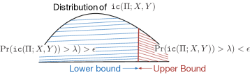
Figure 1: Illustration of lower and upper bounds for $D_{\varepsilon}\left(\pi\right)$

Amortized regime: second-order asymptotics. Denote by $\pi^{n}$ the $n$-fold product protocol obtained by applying $\pi$ to each coordinate $(X_{i},Y_{i})$ for inputs $X^{n}$ and $Y^{n}$. Consider the communication complexity $D_{\varepsilon}(\pi^{n})$ of $\varepsilon$-simulating $\pi^{n}$ for independent and identically distributed (IID) $(X^{n},Y^{n})$ generated from $\mathrm{P}_{XY}^{n}$. Using the bounds above, we can obtain the following sharpening of the results of [8]: With $\mathtt{V}(\pi)$ denoting the variance of $\mathtt{ic}(\Pi;X,Y)$,

$$D_{\varepsilon}(\pi^{n})=n\mathtt{IC}(\pi)+\sqrt{n\mathtt{V}(\pi)}Q^{-1}(\varepsilon)+o(\sqrt{n}),$$

where $Q(x)$ is equal to the probability that a standard normal random variable exceeds $x$ and $Q^{-1}(\varepsilon)\approx\sqrt{\log(1/\varepsilon)}$. On the other hand, the arguments in [8] or [55] give us

$$D_{\varepsilon}(\pi^{n})\geq n\mathtt{IC}(\pi)-n\varepsilon[|\pi|+\log|{\mathcal{X}}||{\mathcal{Y}}|]-\varepsilon\log(1/\varepsilon).$$

But the precise communication requirement is not less but $\sqrt{n\mathtt{V}(\pi)\log(1/\varepsilon)}$ more than $n\mathtt{IC}(\pi)$.

General formula for amortized communication complexity. The lower and upper bounds above can be used to derive a formula for the first-order asymptotic term, the coefficient of $n$, in $D_{\varepsilon}(\pi_{n})$ for any sequence of protocols $\pi_{n}$ with inputs $X_{n}\in{\mathcal{X}}^{n}$ and $Y_{n}\in{\mathcal{Y}}^{n}$ generated from any sequence of distributions $\mathrm{P}_{X_{n}Y_{n}}$. We illustrate our result by the following example.

Example 1 (Mixed protocol).

Consider two protocols $\pi_{\mathtt{h}}$ and $\pi_{\mathtt{t}}$ with inputs $X$ and $Y$ such that $\mathtt{IC}(\pi_{\mathtt{h}})>\mathtt{IC}(\pi_{\mathtt{t}})$. For $n$ IID observations $(X^{n},Y^{n})$ drawn from $\mathrm{P}_{XY}$, we seek to simulate the mixed protocol $\pi_{\mathtt{mix,n}}$ defined as follows: Party 1 first flips a (private) coin with probability $p$ of heads and sends the outcome $\Pi_{0}$ to Party 2. Depending on the outcome of the coin, the parties execute $\pi_{\mathtt{h}}$ or $\pi_{\mathtt{t}}$ $n$ times, i.e., they use $\pi_{\mathtt{h}}^{n}$ if $\Pi_{0}=\mathtt{h}$ and $\pi_{\mathtt{t}}^{n}$ if $\Pi_{0}=\mathtt{t}$. What is the amortized communication complexity of simulating the mixed protocol $\pi_{\mathtt{mix,n}}$? Note that

$$\mathtt{IC}(\pi_{\mathtt{mix,n}})=n\left[p\mathtt{IC}(\pi_{\mathtt{h}})+(1-p)\mathtt{IC}(\pi_{\mathtt{t}})\right].$$

Is it true that in the manner of [8] the leading asymptotic term in $D_{\varepsilon}(\pi_{\mathtt{mix,n}})$ is $\mathtt{IC}(\pi_{\mathtt{mix,n}})$? In fact, it is not so. Our general formula implies that for all $p\in(0,1)$,

$$D_{\varepsilon}(\pi_{\mathtt{mix,n}})=n\mathtt{IC}(\pi_{\mathtt{h}})+o(n)$$

This is particularly interesting when $p$ is very small and $\mathtt{IC}(\pi_{\mathtt{h}})\gg\mathtt{IC}(\pi_{\mathtt{t}})$.

I-B Proof techniques

Proof for the lower bound. We present a new method for deriving lower bounds on distributional communication complexity. Our proof relies on a reduction argument that utilizes an $\varepsilon$-simulation to generate an information theoretically secure secret key for $X$ and $Y$ (for a definition of the latter, see [33, 1] or Section IV). Heuristically, a protocol can be simulated using fewer bits of communication than its length because of the correlation in $X$ and $Y$. Due to this correlation, when simulating the protocol, the parties agree on more bits (generate more common randomness) than what they communicate. These extra bits can be extracted as an information theoretically secure secret key for the two parties using the leftover hash lemma ($cf.$ [6, 43]). A lower bound on the number of bits communicated can be derived using an upper bound for the maximum possible length of a secret key that can be generated using interactive communication; the latter was derived recently in [50, 51].

Protocol for the upper bound. We simulate a given protocol one round at a time. Simulation of each round consists of two subroutines: Interactive Slepian-Wolf compression and message reduction by public randomness. The first subroutine is an interactive version of the classical Slepian-Wolf compression [45] for sending $X$ to an observer of $Y$ which is of optimal instantaneous rate. The second subroutine uses an idea that appeared first in [41] (see, also, [35, 54]) and reduces the number of bits communicated in the first by realizing a portion of the required communication by the shared public randomness. This is possible since we are not required to recover a given random variable $\Pi$, but only simulate it to within a fixed statistical distance.

The proposed protocol is closely related to that in [8]. However, there are some crucial differences. The protocol in [8], too, uses public randomness to sample each round of the protocol, before transmitting it using an interactive communication of size incremented in steps. However, our information theoretic approach provides a systematic method for choosing this step size. Furthermore, our protocol for sampling the protocol from public randomness is significantly different from that in [8] and relies on randomness extraction techniques. In particular, the protocol in [8] does not attain the asymptotically optimal bounds achieved by our protocol.

Technical approach. While we utilize new, bespoke techniques for deriving our lower and upper bounds, casting our problem in an information theoretic framework allows us to build upon the developments in this classic field. In particular, we rely on the information spectrum approach of Han and Verdú, introduced in the seminal paper [23] (see the textbook [22] for a detailed account). In this approach, the classical measures of information such as entropy and mutual information are viewed as expectations of the corresponding information densities, and the notion of “typical sets” is replaced by sets where these information densities are bounded uniformly. The distribution of an information density (such as $h(x)=-\log\mathrm{P}_{X}\left(x\right)$), or the support of this distribution, is loosely referred to as its spectrum. Further, we shall refer to the difference between $\max$ and $\min$ value of $h(x)$ over its support as the length of the spectrum. Coding theorems of classical information theory consider IID repetitions and rely on the so-called the asymptotic equipartition property [12] which essentially corresponds to the concentration of spectrums on small intervals. For single-shot problems such concentrations are not available and we have to work with the whole span of the spectrum.

Our main technical contribution in this paper is the extension of the information spectrum method to handle interactive communication. Our results rely on the analysis of appropriately chosen information densities and, in particular, rely on the spectrum of the information complexity density $\mathtt{ic}(\Pi;X,Y)$. Different components of our analysis require bounds on these information densities in different directions, which in turn renders our bounds loose and incurs a gap equal to the length of the corresponding information spectrum. To overcome this shortcoming, we use the spectrum slicing technique of Han [22] to divide the information spectrum into small portions with information densities closely bounded from both sides. While in our upper bounds spectrum slicing is used to carefully choose the parameters of the protocol, it is required in our lower bounds to identify a set of inputs where a given simulation will require a large number of bits to be communicated.

I-C Organization

A formal statement of the problem along with the necessary preliminaries is given in the next section. Section III contains all our results. In Section IV, we review the information theoretic secret key agreement problem, the leftover hash lemma, and the data exchange problem, all of which will be instrumental in our proofs. The formal proof of our lower bound is contained in Section V and that of our upper bound in Section VI. Section VII contains a proof of our asymptotic results, followed by concluding remarks in Section VIII.

I-D Notations

Random variables are denoted by capital letters such as $X$, $Y$, $etc.$ realizations by small letters such as $x$, $y$, $etc.$ and their range sets by corresponding calligraphic letters such as ${\mathcal{X}}$, ${\mathcal{Y}}$, $etc.$. Protocols are denoted by appropriate subscripts or superscripts with $\pi$, the corresponding random transcripts by the same sub- or superscripts with $\Pi$; $\tau$ is used as a placeholder for realizations of random transcripts. All the logarithms in this paper are to the base $2$.

The following convention, described for the entropy density, shall be used for all information densities used in this paper. We shall abbreviate the entropy density $h_{\mathrm{P}_{X}}(x)=-\log\mathrm{P}_{X}\left(x\right)$ by $h(x)$, when there is no confusion about $\mathrm{P}_{X}$, and the random variable $h(X)$ corresponds to drawing $X$ from the distribution $\mathrm{P}_{X}$.

Whenever there is no confusion, we will not display the dependence of distributional communication complexity on the underlying distribution; the latter remains fixed in most of our discussion.

II Problem Statement

Two parties observe correlated random variables $X$ and $Y$, with Party 1 observing $X$ and Party 2 observing $Y$, generated from a fixed distribution $\mathrm{P}_{XY}$ and taking values in finite sets ${\mathcal{X}}$ and ${\mathcal{Y}}$, respectively. An interactive protocol $\pi$ (for these two parties) consists of shared public randomness $U$, private randomness $U_{\mathcal{X}}$ and $U_{\mathcal{Y}}$, and interactive communication $\Pi_{1},\Pi_{2},...,\Pi_{r}$. The parties communicate alternatively with Party 1 transmitting in the odd rounds and Party 2 in the even rounds. Specifically, in each round $i$ one of the party, say Party 1, communicates and transmits a string of bits $\Pi_{i}\in\{0,1\}^{*}$ determined by the previous transmissions $\Pi_{1},...,\Pi_{i-1}$ and the observations $(X,U_{\mathcal{X}},U)$ of the communicating party. To each possible value of the bit string $\Pi_{i}$, a state from the state space $\{{\tt C},\phi\}$ is associated. If the next state is ${\tt C}$, the other party starts communicating. If it is $\phi$, the protocol stops and each party generates an output based on its local observation and trascript $\Pi_{1},...,\Pi_{i}$ of the protocol. We assume without loss of generality that Party 1 initiates the protocol. Note that the set ${\mathcal{C}}_{i}$ of possible values of $\Pi_{i}$, and the associated next states ${\tt C}$ or $\phi$ for each value, is determined by a common function of $(X,U_{\mathcal{X}},U,\Pi^{i-1})$ and $(Y,U_{\mathcal{Y}},U,\Pi^{i-1})$ ($cf.$ [19]), $i.e.$, as a function of a random variable $V$ such that

$$H(V|X,U_{\mathcal{X}},U,\Pi^{i-1})=H(V|Y,U_{\mathcal{Y}},U,\Pi^{i-1})=0.$$

We denote the overall transcript of the protocol by $\Pi$. The length of a protocol $\pi$, $|\pi|$, is the maximum number of bits that are communicated in any execution of the protocol.

In the special case where ${\mathcal{C}}_{i}$ is a prefix-free set determined by $\Pi^{i-1}$, the protocol is called a tree-protocol ($cf.$ [53, 29]). In this case, the set of transcripts of the protocol can be represented by a tree, termed the protocol tree, with each leaf corresponding to a particular realization of the transcript. Specifically, the protocol is defined by a binary tree where each internal node $v$ is owned by either party, and node $v$ is labeled either by a function $a_{v}:{\mathcal{X}}\times{\mathcal{U}}_{\mathcal{X}}\times{\mathcal{U}}\to\{0,1\}$ or $b_{v}:{\mathcal{Y}}\times{\mathcal{U}}_{\mathcal{Y}}\times{\mathcal{U}}\to\{0,1\}$. Then each leaf, or the path from the root to the leaf, corresponds to the overall transcript. Our proposed protocol is indeed a tree protocol. On the other hand, our converse bound applies to the more general class of interactive protocols described above.

A random variable $F$ is said to be recoverable by $\pi$ for Party 1 (or Party 2) if $F$ is function of $(X,U,U_{\mathcal{X}},\Pi)$ (or $(Y,U,U_{\mathcal{Y}},\Pi)$).

A protocol with a constant $U$ is called a private coin protocol, with a constant $(U_{\mathcal{X}}$, $U_{\mathcal{Y}})$ is called a public coin protocol, and with $(U,U_{\mathcal{X}},U_{\mathcal{Y}})$ constant is called a deterministic protocol. Note that a private coin protocol can be realized as a public coin protocol by sampling private coins from public coins.

When we execute the protocol $\pi$ above, the overall view of the parties consists of random variables $(XY\Pi\Pi)$, where the two $\Pi$s correspond to the transcript of the protocol seen by the two parties. A simulation of the protocol consists of another protocol which generates almost the same view as that of the original protocol. We are interested in the simulation of private coin protocols, using arbitrary protocols; public coin protocols can be simulated by simulating for each fixed value of public randomness the resulting private coin protocol.

Definition 2 ($\varepsilon$-Simulation of a protocol).

Let $\pi$ be a private coin protocol. Given $0\leq\varepsilon<1$, a protocol $\pi_{\mathtt{sim}}$ constitutes an $\varepsilon$-simulation of $\pi$ if there exist $\Pi_{{\mathcal{X}}}$ and $\Pi_{{\mathcal{Y}}}$, respectively, recoverable by $\pi_{\mathtt{sim}}$ for Party 1 and Party 2 such that

$$d_{\mathtt{var}}\left(\mathrm{P}_{\Pi\Pi XY},\mathrm{P}_{\Pi_{{\mathcal{X}}}\Pi_{{\mathcal{Y}}}XY}\right)\leq\varepsilon,$$ (1)

where $d_{\mathtt{var}}\left(\mathrm{P},\mathrm{Q}\right)=\frac{1}{2}\sum_{x}|\mathrm{P}_{x}-\mathrm{Q}_{x}|$ denotes the variational or the statistical distance between $\mathrm{P}$ and $\mathrm{Q}$.

Definition 3 (Distributional communication complexity).

The $\varepsilon$-error distributional communication complexity $D_{\varepsilon}\left(\pi|\mathrm{P}_{XY}\right)$ of simulating a private coin protocol $\pi$ is the minimum length of an $\varepsilon$-simulation of $\pi$. The distribution $\mathrm{P}_{XY}$ remains fixed throughout our analysis; for brevity, we shall abbreviate $D_{\varepsilon}\left(\pi|\mathrm{P}_{XY}\right)$ by $D_{\varepsilon}\left(\pi\right)$.

Problem. Given a protocol $\pi$ and a joint distribution $\mathrm{P}_{XY}$ for the observations of the two parties, we seek to characterize $D_{\varepsilon}\left(\pi\right)$.

Remark 1 (Deterministic protocols).

Note that a deterministic protocol corresponds to an interactive function. A specific instance of this situation appears in [49] where $\Pi(X,Y)=(X,Y)$ is considered. For such protocols,

$$d_{\mathtt{var}}\left(\mathrm{P}_{\Pi\Pi XY},\mathrm{P}_{\Pi_{{\mathcal{X}}}\Pi_{{\mathcal{Y}}}XY}\right)=1-{\mathrm{Pr}}\left(\Pi=\Pi_{{\mathcal{X}}}=\Pi_{{\mathcal{Y}}}\right).$$

Therefore, a protocol is an $\varepsilon$-simulation of a deterministic protocol if and only if it computes the corresponding interactive function with probability of error less than $\varepsilon$. Furthermore, randomization does not help in this case, and it suffices to use deterministic simulation protocols. Thus, our results below provide tight bounds for distributional communication complexity of interactive functions and even of all functions which are information theoretically securely computable for the distribution $\mathrm{P}_{XY}$, since computing these functions is tantamount to computing an interactive function [36] (see, also, [5, 28]).

Remark 2 (Compression of protocols).

A protocol $\pi_{\mathtt{com}}$ constitutes an $\varepsilon$-compression of a given protocol $\pi$ if it recovers $\Pi_{\mathcal{X}}$ and $\Pi_{\mathcal{Y}}$ for Party 1 and Party 2 such that

$${\mathrm{Pr}}\left(\Pi=\Pi_{\mathcal{X}}=\Pi_{\mathcal{Y}}\right)\geq 1-\varepsilon.$$

Note that randomization does not help in this case either. In fact, for deterministic protocols simulation and compression coincide. In general, however, compression is a more demanding task than simulation and our results show that in many cases, (such as the amortized regime), compression requires strictly more communication than simulation. Specifically, our results for $\varepsilon$-simulation in this paper can be modified to get corresponding results for $\varepsilon$-compression by replacing the information complexity density $\mathtt{ic}(\tau;x,y)$ by

$$h(\tau|x)+h(\tau|y)=-\log\mathrm{P}_{\Pi|X}\left(\tau|x\right)\mathrm{P}_{\Pi|Y}\left(\tau|y\right).$$

The proofs remain essentially the same and, in fact, simplify significantly.

III Main Results

We derive a lower bound for $D_{\varepsilon}\left(\pi\right)$ which applies to all private coin protocols $\pi$ and, in fact, applies to the more general problem of communication complexity of sampling a correlated random variable. For protocols with bounded number of rounds of interaction, admittedly a significant restriction, $i.e.$, protocols with $r=r(X,Y,U,U_{\mathcal{X}},U_{\mathcal{Y}})\leq r_{\max}$ with probability $1$, we present a simulation protocol which yields upper bounds for $D_{\varepsilon}\left(\pi\right)$ of similar form as our lower bounds. In particular, in the asymptotic regime our bounds improve over previously known bounds and are tight.

III-A Lower bound

We prove the following lower bound.

Theorem 1.

Given $0\leq\varepsilon<1$ and a protocol $\pi$, for arbitrary $0<\eta<1/3$

$$D_{\varepsilon}\left(\pi\right)\geq\sup\{\lambda:{\mathrm{Pr}}\left(\mathtt{ic}(\Pi;X,Y)>\lambda\right)\geq\varepsilon+\varepsilon^{\prime}\}-\lambda^{\prime},$$ (2)

where the fudge parameters $\varepsilon^{\prime}$ and $\lambda^{\prime}$ depend on $\eta$ as well as appropriately chosen information spectrums and will be described below in (4) and (5).

The appearance of fudge parameters such as $\varepsilon^{\prime}$ and $\lambda^{\prime}$ in the bound above is typical since the techniques to bound the tail probability of random variables invariably entail such parameters, which are tuned based on the specific scenario being studied. For instance, the Chernoff bound has a parameter that is tuned with respect to the moment generating function of the random variable of interest. More relevant to the problem studied here, such fudge parameters also show up in the evalutation of error probability of single-party non-interactive compression problems ($cf.$ [23, 22]).

When the fudge parameters $\varepsilon^{\prime}$ and $\lambda^{\prime}$ are negligible, the right-side of the bound above is close to the $\varepsilon$-tail of $\mathtt{ic}(\Pi;X,Y)$. Indeed, the fudge parameters turn out to be negligible in many cases of interest. For instance, for the amortized case $\varepsilon^{\prime}$ can be chosen to be arbitrarily small. The parameter $\lambda^{\prime}$ is related to the length of the interval in which the underlying information densities lie with probability greater than $1-\varepsilon^{\prime}$, the essential length of spectrums. For the amortized case with product protocols, by the central limit theorem the related essential spectrums are of length $\Lambda={\mathcal{O}}(\sqrt{n})$ and $\lambda^{\prime}=\log\Lambda$. On the other hand, $\lambda_{\varepsilon}$ is ${\mathcal{O}}(n)$. Thus, the $\log n$ order fudge parameter $\lambda^{\prime}$ is negligible in this case. The same is true also for the example protocol in Appendix A. Finally, it should be noted that similar fudge parameters are ubiquitous in single-shot bounds; for instance, see [22, Lemma 1.3.2].

Remark 3.

The result above does not rely on the interactive nature of $\Pi$ and is valid for simulation of any random variable $\Pi$. Specifically, for any joint distribution $\mathrm{P}_{\Pi XY}$, an $\varepsilon$-simulation satisfying (1) must communicate at least as many bits as the right-side of (2), which is roughly equal to the largest value $\lambda_{\varepsilon}$ of $\lambda$ such that ${\mathrm{Pr}}\left(\mathtt{ic}(\Pi;X,Y)>\lambda\right)>\varepsilon$.

The fudge parameters. The fudge parameters $\varepsilon^{\prime}$ and $\lambda^{\prime}$ in Theorem 1 depend on the spectrums of the following information densities:

1. Information complexity density: This density is described in Definition 1 and will play a pivotal role in our results.

2. Entropy density of $(X,Y)$: This density, given by $h(X,Y)=-\log\mathrm{P}_{XY}\left(X,Y\right)$, captures the randomness in the data and plays a fundamental role in the compression of the collective data of the two parties ($cf.$ [22]).

3. Conditional entropy density of $X$ given $Y\Pi$: The conditional entropy density $h(X|Y)=-\log\mathrm{P}_{X|Y}\left(X|Y\right)$ plays a fundamental role in the compression of $X$ for an observer of $Y$ [34, 22]. We shall use the conditional entropy density $h(X|Y\Pi)$ in our bounds.

4. Sum conditional entropy density of $(X\Pi,Y\Pi)$: The sum conditional entropy density is given by $h\left(X\triangle Y\right)=-\log\mathrm{P}_{X|Y}\left(X|Y\right)\mathrm{P}_{Y|X}\left(Y|X\right)$ has been shown recently to play a fundamental role in the communication complexity of the data exchange problem [49]. We shall use the sum conditional entropy density $h\left(X\Pi\triangle Y\Pi\right)$.

5. Information density of $X$ and $Y$ is given by $i(X\wedge Y)\stackrel{{\scriptstyle{\rm def}}}{{=}}h(X)-h(X|Y)$.

Let $[\lambda_{\min}^{(1)},\lambda_{\max}^{(1)}]$, $[\lambda_{\min}^{(2)},\lambda_{\max}^{(2)}]$, and $[\lambda_{\min}^{(3)},\lambda_{\max}^{(3)}]$ denote the “essential” spectrums of information densities $\zeta_{1}=h(X,Y)$, $\zeta_{2}=h(X|Y\Pi)$, and $\zeta_{3}=h\left(X\Pi\triangle Y\Pi\right)$, respectively. Concretely, let the tail events ${\mathcal{E}}_{i}=\{\zeta_{i}\notin[\lambda_{\min}^{(i)},\lambda_{\max}^{(i)}]\}$, $i=1,2,3$, satisfy

$${\mathrm{Pr}}\left({\mathcal{E}}_{1}\right)+{\mathrm{Pr}}\left({\mathcal{E}}_{2}\right)+{\mathrm{Pr}}\left({\mathcal{E}}_{3}\right)\leq\varepsilon_{\mathtt{tail}},$$ (3)

where $\varepsilon_{\mathtt{tail}}$ can be chosen to be appropriately small. Further, let $\Lambda_{i}=\lambda_{\max}^{(i)}-\lambda_{\min}^{(i)}$, $i=1,2,3$, denote the corresponding effective spectrum lengths. The parameters $\varepsilon^{\prime}$ and $\lambda^{\prime}$ in Theorem 1 are given by

$$\varepsilon^{\prime}=\varepsilon_{\mathtt{tail}}+2\eta$$ (4)

and

$$\lambda^{\prime}=2\log\Lambda_{1}\Lambda_{3}+\log\Lambda_{2}-\log(1-3\eta)+9\log 1/\eta+3,$$ (5)

where $0<\eta<1/3$ is arbitrary. If $\Lambda_{i}=0$, $i=1,2,3$, we can replace it with $1$ in the bound above. Thus, our spectrum slicing approach allows us to reduce the dependence of $\lambda^{\prime}$ on spectrum lengths $\Lambda_{i}$’s from linear to logarithmic.

III-B Upper bound

We prove the following upper bound.

Theorem 2.

For every $0\leq\varepsilon<1$ and every protocol $\pi$,

$$D_{\varepsilon}\left(\pi\right)\leq\inf\left\{\lambda:{\mathrm{Pr}}\left(\mathtt{ic}(\Pi;X,Y)>\lambda\right)\leq\varepsilon-\varepsilon^{\prime}\right\}+\lambda^{\prime},$$

where the fudge parameters $\varepsilon^{\prime}$ and $\lambda^{\prime}$ depend on the maximum number of rounds of interaction in $\pi$ and on appropriately chosen information spectrums.

Remark 4.

In contrast to the lower bound given in the previous section, the upper bound above relies on the interactive nature of $\pi$. Furthermore, the fudge parameters $\varepsilon^{\prime}$ and $\lambda^{\prime}$ depend on the number of rounds, and the upper bound may not be useful when the number of rounds is not negligible compared to the $\varepsilon$-tail of the information complexity density. However, we will see that the above upper bound is tight for the amortized regime, even up to the second-order asymptotic term.

The simulation protocol. Our simulation protocol simulates the given protocol $\pi$ round-by-round, starting from $\Pi_{1}$ to $\Pi_{r}$. Simulation of each round consists of two subroutines: Interactive Slepian-Wolf compression and message reduction by public randomness.

The first subroutine uses an interactive version of the classical Slepian-Wolf compression [45] (see [34] for a single-shot version) for sending $X$ to an observer of $Y$. The standard (noninteractive) Slepian-Wolf coding entails hashing $X$ to $l$ values and sending the hash values to the observer of $Y$. The number of hash values $l$ is chosen to take into account the worst-case performance of the protocol. However, we are not interested in the worst-case performance of each round, but of the overall multiround protocol. As such, we seek to compress $X$ using the least possible instantaneous rate. To that end, we increase the number of hash values gradually, $\Delta$ at a time, until the receiver decodes $X$ and sends back an ACK. We apply this subroutine to each round $i$, say $i$ odd, with $\Pi_{i}$ in the role of $X$ and $(Y,\Pi_{1}....,\Pi_{i-1})$ in the role of $Y$. Similar interactive Slepian-Wolf compression schemes have been considered earlier in different contexts ($cf.$  [17, 38, 52, 25, 49]).

The second subroutine reduces the number of bits communicated in the first by realizing a portion of the required communication by the shared public randomness $U$. Specifically, instead of transmitting hash values of $\Pi_{i}$, we transmit hash values of a random variable $\hat{\Pi}_{i}$ generated in such a manner that some of its corresponding hash bits can be extracted from $U$ and the overall joint distributions do not change by much. Since $U$ is independent of $(X,Y)$, the number $k$ of hash bits that can be realized using public randomness is the maximum number of random hash bits of $\Pi_{i}$ that can be made almost independent of $(X,Y)$, a good bound for which is given by the leftover hash lemma. The overall simulation protocol for $\Pi_{i}$ now communicates $l-k$ instead of $l$ bits. A similar technique for message reduction appears in a different context in [41, 35, 54].

The overall performance of the protocol above is still suboptimal because the saving of $k$ bits is limited by the worst-case performance. To remedy this shortcoming, we once again take recourse to spectrum slicing to ensure that our saving $k$ is close to the best possible for each realization $(\Pi,X,Y)$.

Note that our protocol above is closely related to that proposed in [8]. However, the information theoretic form here makes it amenable to techniques such as spectrum slicing, which leads to tighter bounds than those established in [8].

The fudge parameters. The fudge parameters $\varepsilon^{\prime}$ and $\lambda^{\prime}$ in Theorem 2 depend on the spectrum of various conditional information densities. To optimize the performance of each subroutine described above, we slice the spectrum of the respective conditional information density involved. Specifically, for odd round $t$, we slice the spectrum of $h(\Pi_{t}|Y\Pi^{t-1})=-\log\mathrm{P}_{\Pi_{t}|Y\Pi^{t-1}}\left(\Pi_{t}|Y,\Pi^{t-1}\right)$ for interactive Slepian-Wolf compression and $h(\Pi_{t}|X\Pi^{t-1})=-\log\mathrm{P}_{\Pi_{t}|X\Pi^{t-1}}\left(\Pi_{t}|X,\Pi^{t-1}\right)$ for the substitution of message by public randomness; for even rounds, the role of $X$ and $Y$ is interchanged. Each round involves some residuals related to the two conditional information densities. The fudge parameters $\varepsilon^{\prime}$ and $\lambda^{\prime}$ are accumulations of the residuals of each round. The explicit expressions for $\varepsilon^{\prime}$ and $\lambda^{\prime}$ are rather technical and are given in Section VI-E along with the proofs.

III-C Amortized regime: second-order asymptotics

It was shown in [8] that information complexity of a protocol equals the amortized communication rate for simulating the protocol, $i.e.$,

$$\lim_{\varepsilon\to 0}\lim_{n\to\infty}\frac{1}{n}D_{\varepsilon}(\pi^{n}|\mathrm{P}_{XY}^{n})=\mathtt{IC}(\pi),$$

where $\mathrm{P}_{XY}^{n}$ denotes the $n$-fold product of the distribution $\mathrm{P}_{XY}$, namely the distribution of random variables $(X_{i},Y_{i})_{i=1}^{n}$ drawn IID from $\mathrm{P}_{XY}$, and $\pi^{n}$ corresponds to running the same protocol $\pi$ on every coordinate $(X_{i},Y_{i})$. Thus, $\mathtt{IC}(\pi)$ is the first-order term (coefficient of $n$) in the communication complexity of simulating the $n$-fold product of the protocol. However, the analysis in [8] sheds no light on finer asymptotics such as the second-order term or the dependence of $D_{\varepsilon}(\pi^{n}|\mathrm{P}_{XY}^{n})$ on $\varepsilon$. On the one hand, it even remains unclear from [8] if a positive $\varepsilon$ reduces the amortized communication rate or not. On the other hand, the amortized communication rate yields only a loose bound for $D_{\varepsilon}(\pi^{n}|\mathrm{P}_{XY}^{n})$ for a finite, fixed $n$. A better estimate of $D_{\varepsilon}(\pi^{n}|\mathrm{P}_{XY}^{n})$ at a finite $n$ and for a fixed $\varepsilon$ can be obtained by identifying the second-order asymptotic term. Such second-order asymptotics were first considered in [46] and have received a lot of attention in information theory in recent years following [24, 39].

Our lower bound in Theorem 1 and upper bound in Theorem 2 show that the leading term in $D_{\varepsilon}(\pi^{n}|\mathrm{P}_{XY}^{n})$ is roughly the $\varepsilon$-tail $\lambda_{\varepsilon}$ of the random variable $\mathtt{ic}(\Pi^{n};X^{n},Y^{n})=\sum_{i=1}^{n}\mathtt{ic}(\Pi_{i};X_{i},Y_{i})$, a sum of $n$ IID random variables. By the central limit theorem the first-order asymptotic term in $\lambda_{\varepsilon}$ equals $n{\mathbb{E}}\left[\mathtt{ic}(\Pi;X,Y)\right]=n\mathtt{IC}(\pi)$, recovering the result of [8]. Furthermore, the second-order asymptotic term depends on the variance $\mathtt{V}(\pi)$ of $\mathtt{ic}(\Pi;X,Y)$, $i.e.$, on

$$\mathtt{V}(\pi)\stackrel{{\scriptstyle{\rm def}}}{{=}}\mathrm{Var}\left[\mathtt{ic}(\Pi;X,Y)\right].$$

We have the following result.

Theorem 3.

For every $0<\varepsilon<1$ and every protocol $\pi$ with $\mathtt{V}(\pi)>0$,

$$D_{\varepsilon}(\pi^{n}|\mathrm{P}_{XY}^{n})=n\mathtt{IC}(\pi)+\sqrt{n\mathtt{V}(\pi)}Q^{-1}(\varepsilon)+o(\sqrt{n}),$$

where $Q(x)$ is equal to the probability that a standard normal random variable exceeds $x$.

As a corollary, we obtain the strong converse.

Corollary 4.

For every $0<\varepsilon<1$, the amortized communication rate

$$\lim_{n\to\infty}\frac{1}{n}D_{\varepsilon}(\pi^{n}|\mathrm{P}_{XY}^{n})=\mathtt{IC}(\pi).$$

Corollary 4 implies that the amortized communication complexity of simulating protocol $\pi$ cannot be smaller than its information complexity even if we allow a positive error. Thus, if the length of the simulation protocol $\pi_{\mathtt{sim}}$ is “much smaller” than $n\mathtt{IC}(\pi)$, the corresponding simulation error $\varepsilon=\varepsilon_{n}$ must approach $1$. But how fast does this $\varepsilon_{n}$ converge to $1$? Our next result shows that this convergence is exponentially rapid in $n$.

Theorem 5.

Given a protocol $\pi$ and an arbitrary $\delta>0$, for any simulation protocol $\pi_{\mathtt{sim}}$ with

$$|\pi_{\mathtt{sim}}|\leq n[\mathtt{IC}(\pi)-\delta],$$

there exists a constant $E=E(\delta)>0$ such that for every $n$ sufficiently large, it holds that

$$d_{\mathtt{var}}\left(\mathrm{P}_{\Pi^{n}\Pi^{n}X^{n}Y^{n}},\mathrm{P}_{\Pi_{{\mathcal{X}}}^{n}\Pi_{{\mathcal{Y}}}^{n}X^{n}Y^{n}}\right)\geq 1-2^{-En}.$$

A similar converse was first shown for the channel coding problem by Arimoto [3] (see [16, 40] for further refinements of this result), and has been studied for other classical information theory problems as well. To the best of our knowledge, Corollary 5 is the first instance of an Arimoto converse for a problem involving interactive communication.

In the theoretical computer science literature, such converse results have been termed direct product theorems and have been considered in the context of the (distributional) communication complexity problem (for computing a given function) [9, 11, 26]. Our lower bound in Theorem 1, too, yields a direct product theorem for the communication complexity problem. We state this simple result in the passing, skipping the details since they closely mimic Theorem 5. Specifically, given a function $f$ on ${\mathcal{X}}\times{\mathcal{Y}}$, by a slight abuse of notations and terminologies, let $D_{\varepsilon}(f)=D_{\varepsilon}(f|\mathrm{P}_{XY})$ be the communication complexity of computing $f$. As noted in Remark 3, Theorem 1 is valid for an arbitrary random variables $\Pi$, and not just an interactive protocol. Then, by following the proof of Theorem 5 with $F=f(X,Y)$ replacing $\Pi$ in the application of Theorem 1, we get the following direct product theorem.

Theorem 6.

Given a function $f$ and an arbitrary $\delta>0$, for any function computation protocol $\pi$ computing estimates $F_{{\mathcal{X}},n}$ and $F_{{\mathcal{Y}},n}$ of $f^{n}$ at the Party 1 and Party 2, respectively, and with length

$$|\pi|\leq n[H(F|X)+H(F|Y)-\delta],$$ (6)

there exists a constant $E=E(\delta)>0$ such that for every $n$ sufficiently large, it holds that

$${\mathrm{Pr}}\left(F_{{\mathcal{X}},n}=F_{{\mathcal{Y}},n}=F^{n}\right)\leq 2^{-En},$$

where $F^{n}:=(F_{1},...,F_{n})$ and $F_{i}:=f(X_{i},Y_{i})$, $1\leq i\leq n$.

Recall that [8, 31] showed that the first order asymptotic term in the amortized communication complexity for function computation equals the information complexity $\mathtt{IC}(f)$ of the function, namely the infimum over $\mathtt{IC}(\pi)$ for all interactive protocols $\pi$ that recover $f$ with $0$ error. Ideally, we would like to show an Arimoto converse for this problem, $i.e.$, replace the threshold on the right-side of (6) with $n[\mathtt{IC}(f)-\delta]$. The direct product result above is weaker than such an Arimoto converse, and proving the Arimoto converse for the function computation problem is work in progress. Nevertheless, the simple result above is not comparable with the known direct product theorems in [9, 11] and can be stronger in some regimes.

III-D General formula for amortized communication complexity

Consider arbitrary distributions $\mathrm{P}_{X_{n}Y_{n}}$ on ${\mathcal{X}}^{n}\times{\mathcal{Y}}^{n}$ and arbitrary protocols $\pi_{n}$ with inputs $X_{n}$ and $Y_{n}$ taking values in ${\mathcal{X}}^{n}$ and ${\mathcal{Y}}^{n}$, for each $n\in{\mathbbm{N}}$. For vanishing simulation error $\varepsilon_{n}$, how does $D_{\varepsilon_{n}}(\pi_{n}|\mathrm{P}_{X_{n}Y_{n}})$ evolve as a function of $n$?

The previous section, and much of the theoretical computer science literature, has focused on the case when $\mathrm{P}_{X_{n}Y_{n}}=\mathrm{P}_{XY}^{n}$ and the same protocol $\pi$ is executed on each coordinate. In this section, we identify the first-order asymptotic term in $D_{\varepsilon_{n}}(\pi_{n}|\mathrm{P}_{X_{n}Y_{n}})$ for a general sequence of distributions $\{\mathrm{P}_{X_{n}Y_{n}}\}_{n=1}^{\infty}$ and a general sequence of protocols $\boldsymbol{\pi}=\{\pi_{n}\}_{n=1}^{\infty}$. Formally, the amortized (distributional) communication complexity of $\boldsymbol{\pi}$ for $\{\mathrm{P}_{X_{n}Y_{n}}\}_{n=1}^{\infty}$ is given by

$$D(\boldsymbol{\pi})\stackrel{{\scriptstyle{\rm def}}}{{=}}\lim_{\varepsilon\to 0}\,\limsup_{n\to\infty}\frac{1}{n}D_{\varepsilon}(\pi_{n}|\mathrm{P}_{X_{n}Y_{n}}).$$

Our goal is to characterize $D(\boldsymbol{\pi})$ for any given sequences $\mathrm{P}_{n}$ and $\boldsymbol{\pi}$. We seek a general formula for $D(\boldsymbol{\pi})$ under minimal assumptions. Since we do not make any assumptions on the underlying distribution, we cannot use any measure concentration results. Instead, we take recourse to probability limits of information spectrums introduced by Han and Verdú in [23] for handling this situation ($cf.$  [22]). Specifically, for a sequence of protocols $\boldsymbol{\pi}=\{\pi_{n}\}_{n=1}^{\infty}$ and a sequence of observations $(\mathbf{X},\mathbf{Y})=\{(X_{n},Y_{n})\}_{n=1}^{\infty}$, the sup information complexity is defined as

$$\overline{\mathtt{IC}}(\boldsymbol{\pi})\stackrel{{\scriptstyle{\rm def}}}{{=}}\inf\left\{\alpha\mid\lim_{n\to\infty}{\mathrm{Pr}}\left(\frac{1}{n}\mathtt{ic}(\Pi_{n};X_{n},Y_{n})>\alpha\right)=0\right\},$$

where, with a slight abuse of notation, $\Pi_{n}$ is the transcript of protocol $\pi_{n}$ for observations $(X_{n},Y_{n})$. The result below shows that it is $n\overline{\mathtt{IC}}(\boldsymbol{\pi})$, and not $\mathtt{IC}(\pi_{n})$, that determines the communication complexity in general.

Theorem 7.

For every sequence of protocols $\boldsymbol{\pi}=\{\pi_{n}\}_{n=1}^{\infty}$,

$$D(\boldsymbol{\pi})=\overline{\mathtt{IC}}(\boldsymbol{\pi}).$$

The proof uses Theorem 1 and Theorem 2 with carefully chosen spectrum-slice sizes.

For the case when $\pi_{n}=\pi^{n}$ and $\mathrm{P}_{X_{n}Y_{n}}=\mathrm{P}_{XY}^{n}$, it follows from the law of large numbers that $\overline{\mathtt{IC}}(\boldsymbol{\pi})=\mathtt{IC}(\pi)$ and we recover the result of [8]. However, the utility of the general formula goes beyond this simple amortized regime. Example 1 provides one such instance. In this case, $\overline{\mathtt{IC}}(\boldsymbol{\pi})$ can be easily shown to equal $\mathtt{IC}(\pi_{\mathtt{h}})$ for any bias of the coin $\Pi_{0}$.

IV Background: Secret Key Agreement and Data Exchange

Our proofs draw from various techniques in cryptography and information theory. In particular, we use our recent results on information theoretic secret key agreement and data exchange, which are reviewed in this section together with the requisite background.

IV-A Secret key agreement by public discussion

The problem of two party secret key agreement by public discussion was alluded to in [7], but a proper formulation and an asymptotically optimal construction appeared first in [33, 1]. Consider two parties with the first and the second party, respectively, observing the random variable $X$ and $Y$. Using an interactive protocol $\pi$ and their local observations, the parties agree on a secret key. A random variable $K$ constitutes a secret key if the two parties form estimates that agree with $K$ with probability close to $1$ and $K$ is concealed, in effect, from an eavesdropper with access to the transcript $\Pi$ and a side-information $Z$. Formally, let $K_{\mathcal{X}}$ and $K_{\mathcal{Y}}$, respectively, be recoverable by $\pi$ for the first and the second party. Such random variables $K_{\mathcal{X}}$ and $K_{\mathcal{Y}}$ with common range ${\mathcal{K}}$ constitute an $\varepsilon$-secret key if the following condition is satisfied:

$$d_{\mathtt{var}}\left(\mathrm{P}_{K_{\mathcal{X}}K_{\mathcal{Y}}\Pi Z},\mathrm{P}_{\mathtt{unif}}^{(2)}\times\mathrm{P}_{\Pi Z}\right) \leq\varepsilon,$$

where

$$\mathrm{P}_{\mathtt{unif}}^{(2)}\left(k_{\mathcal{X}},k_{\mathcal{Y}}\right)=\frac{\mathbbm{1}(k_{\mathcal{X}}=k_{\mathcal{Y}})}{|{\mathcal{K}}|}.$$

The condition above ensures both reliable recovery, requiring ${\mathrm{Pr}}\left(K_{\mathcal{X}}\neq K_{\mathcal{Y}}\right)$ to be small, and information theoretic secrecy, requiring the distribution of $K_{\mathcal{X}}$ (or $K_{\mathcal{Y}}$) to be almost independent of the eavesdropper’s side information $(\Pi,Z)$ and to be almost uniform. See [50] for a discussion.

Definition 4.

Given $0\leq\varepsilon<1$, the supremum over lengths $\log|{\mathcal{K}}|$ of an $\varepsilon$-secret key is denoted by $S_{\varepsilon}(X,Y|Z)$, and for the case when $Z$ is constant by $S_{\varepsilon}(X,Y)$.

By its definition, $S_{\varepsilon}(X,Y|Z)$ has the following monotonicity property.

Lemma 8 (Monotonicity).

For any deterministic protocol $\pi$,

$$S_{\varepsilon}(X,Y|Z)\geq S_{\varepsilon}(X\Pi,Y\Pi|Z\Pi).$$

Furthermore, if $V_{\mathcal{X}}$ and $V_{\mathcal{Y}}$ can be recovered by $\pi$ for the first and the second party, respectively, then

$$S_{\varepsilon}(X,Y|Z)\geq S_{\varepsilon}(XV_{\mathcal{X}},V_{\mathcal{Y}}|Z\Pi).$$

The claim holds since the two parties can generate a secret key by first running $\pi$ and then generating a secret key for the case when the first party observes $(X,\Pi)$, the second party observes $(Y,\Pi)$ and the eavesdropper observes $(Z,\Pi)$. Similarly, the second inequality holds since the parties can ignore a portion of their observations and generate a secret key from $(X,V_{\mathcal{X}})$ and $(Y,V_{\mathcal{Y}})$.

IV-A1 Leftover hash lemma

A key tool for generating secret keys is the leftover hash lemma ($cf.$ [42]) which, given a random variable $X$ and an $l$-bit eavesdropper’s observation $Z$, allows us to extract roughly $H_{\min}(\mathrm{P}_{X})-l$ bits of uniform bits, independent of $Z$. We shall use a slightly more general form. Given random variables $X$ and $Z$, let

$$H_{\min}\left(\mathrm{P}_{XZ}\mid\mathrm{Q}_{Z}\right)\stackrel{{\scriptstyle{\rm def}}}{{=}}\sup_{x,z}-\log\frac{\mathrm{P}_{XZ}\left(x,z\right)}{\mathrm{Q}_{Z}\left(z\right)}.$$

We define the conditional min-entropy of $X$ given $Z$ as

$$H_{\min}\left(\mathrm{P}_{XZ}\mid Z\right)\stackrel{{\scriptstyle{\rm def}}}{{=}}\sup_{\mathrm{Q}_{Z}\,:\,\mathtt{supp}(\mathrm{P}_{Z})\,\subset\,\mathtt{supp}(\mathrm{Q}_{Z})}H_{\min}\left(\mathrm{P}_{XZ}\mid\mathrm{Q}_{Z}\right).$$

Further, let ${\mathcal{F}}$ be a 2-universal family of mappings $f:{\mathcal{X}}\rightarrow{\mathcal{K}}$, $i.e.$, for each $x^{\prime}\neq x$, the family ${\mathcal{F}}$ satisfies

$$\frac{1}{|{\mathcal{F}}|}\sum_{f\in{\mathcal{F}}}\mathbbm{1}(f(x)=f(x^{\prime}))\leq\frac{1}{|{\mathcal{K}}|}.$$

Lemma 9 (Leftover Hash).

Consider random variables $X,Z$ and $V$ taking values in countable sets ${\mathcal{X}}$, ${\mathcal{Z}}$, and a finite set ${\mathcal{V}}$, respectively. Let $S$ be a random seed such that $f_{S}$ is uniformly distributed over a 2-universal family ${\mathcal{F}}$. Then, for $K_{S}=f_{S}(X)$

$${\mathbb{E}}_{S}\left\{{d_{\mathtt{var}}\left(\mathrm{P}_{K_{S}VZ},\mathrm{P}_{\mathtt{unif}}\mathrm{P}_{VZ}\right)}\right\}\leq\frac{1}{2}\sqrt{|{\mathcal{K}}||{\mathcal{V}}|2^{-H_{\min}\left(\mathrm{P}_{XZ}\mid Z\right)}},$$

where $\mathrm{P}_{\mathtt{unif}}$ is the uniform distribution on ${\mathcal{K}}$.

The version above is a straightforward modification of the leftover hash lemma in, for instance, [42] and can be derived in a similar manner.

As an application of the leftover hash lemma above, we get the following useful result.

Lemma 10.

Consider random variables $X,Y,Z$ and $V$ taking values in countable sets ${\mathcal{X}}$, ${\mathcal{Y}}$, ${\mathcal{Z}}$, and a finite set ${\mathcal{V}}$, respectively. Then,

$$S_{2\varepsilon}(X,Y|ZV)\geq S_{\varepsilon}(X,Y|Z)-\log|{\mathcal{V}}|-2\log(1/2\varepsilon).$$

The proof is relegated to Appendix B.

IV-A2 Conditional independence testing upper bound for secret key lengths

Next, we recall the conditional independence testing upper bound for $S_{\varepsilon}(X,Y)$, which was established in [50, 51]. In fact, the general upper bound in [50, 51] is a single-shot upper bound on the secret key length for a multiparty secret key agreement problem with side information at the eavesdropper. Below, we recall a specialization of the general result for the two party case with no side information at the eavesdropper. In order to state the result, we need the following concept from binary hypothesis testing.

Consider a binary hypothesis testing problem with null hypothesis $\mathrm{P}$ and alternative hypothesis $\mathrm{Q}$, where $\mathrm{P}$ and $\mathrm{Q}$ are distributions on the same alphabet ${\cal V}$. Upon observing a value $v\in{\mathcal{V}}$, the observer needs to decide if the value was generated by the distribution $\mathrm{P}$ or the distribution $\mathrm{Q}$. To this end, the observer applies a stochastic test $\mathrm{T}$, which is a conditional distribution on $\{0,1\}$ given an observation $v\in{\mathcal{V}}$. When $v\in{\mathcal{V}}$ is observed, the test $\mathrm{T}$ chooses the null hypothesis with probability $\mathrm{T}(0|v)$ and the alternative hypothesis with probability $T(1|v)=1-T(0|v)$. For $0\leq\varepsilon<1$, denote by $\beta_{\varepsilon}(\mathrm{P},\mathrm{Q})$ the infimum of the probability of error of type II given that the probability of error of type I is less than $\varepsilon$, $i.e.$,

$$\beta_{\varepsilon}(\mathrm{P},\mathrm{Q}):=\inf_{\mathrm{T}\,:\,\mathrm{P}[\mathrm{T}]\geq 1-\varepsilon}\mathrm{Q}[\mathrm{T}],$$

where

$$\mathrm{P}[\mathrm{T}] = \sum_{v}\mathrm{P}(v)\mathrm{T}(0|v),$$

$$\mathrm{Q}[\mathrm{T}] = \sum_{v}\mathrm{Q}(v)\mathrm{T}(0|v).$$

The following upper bound for $S_{\varepsilon}(X,Y)$ was established in [50, 51].

Theorem 11 (Conditional independence testing bound).

Given $0\leq\varepsilon<1$, $0<\eta<1-\varepsilon$, the following bound holds:

$$S_{\varepsilon}\left(X,Y\right)\leq-\log\beta_{\varepsilon+\eta}\big{(}\mathrm{P}_{XY},\mathrm{Q}_{X}\mathrm{Q}_{Y}\big{)}+2\log(1/\eta),$$

for all distributions $\mathrm{Q}_{X}$ and $\mathrm{Q}_{Y}$ on ${\mathcal{X}}$ and ${\mathcal{Y}}$, respectively.

We close by noting a further upper bound for $\beta_{\varepsilon}(\mathrm{P},\mathrm{Q})$, which is easy to derive.

Lemma 12.

For every $0\leq\varepsilon<1$ and $\lambda$,

$$-\log\beta_{\varepsilon}(\mathrm{P},\mathrm{Q})\leq\lambda-\log\left(\mathrm{P}\left(\log\frac{\mathrm{P}\left(X\right)}{\mathrm{Q}\left(X\right)}<\lambda\right)-\varepsilon\right)_{+},$$

where $(x)_{+}=\max\{0,x\}$. As a corollary, we obtain the following upper bound for $S_{\varepsilon}(X,Y)$:

$$S_{\varepsilon}\left(X,Y\right)\leq\lambda-\log\left({\mathrm{Pr}}\left(\log\frac{\mathrm{P}_{XY}\left(X,Y\right)}{\mathrm{Q}_{X}\left(X\right)\mathrm{Q}_{Y}\left(Y\right)}<\lambda\right)-\varepsilon-\eta\right)_{+}+2\log(1/\eta),$$

for all distributions $\mathrm{Q}_{X}$ and $\mathrm{Q}_{Y}$.

IV-B The data exchange problem

The next primitive that will be used in the reduction argument in our lower bound proof is a protocol for data exchange. The parties observing $X$ and $Y$ seek to know each other’s data. What is the minimum length of interactive communication required? This basic problem, first studied in [37], is in effect a two-party extension of the classical Slepian-Wolf compression [45] (see [14] for a multiparty version). In a recent work [49], we derived tight lower and upper bounds for the length of a protocol that, for a given distribution $\mathrm{P}_{XY}$, will facilitate data exchange with probability of error less than $\varepsilon$. We review the proposed protocol and its performance here; first, we formally define the data exchange problem.

Definition 5.

For $0\leq\varepsilon<1$, a protocol $\pi$ attains $\varepsilon$-data exchange if there exist $\hat{Y}$ and $\hat{X}$ which are recoverable by $\pi$ for the first and the second party, respectively, and satisfy

$$\mathrm{P}(\hat{X}=X,~{}\hat{Y}=Y)\geq 1-\varepsilon.$$

Note that data exchange corresponds to simulating a (deterministic) interactive protocol $\pi$ where $\Pi_{1}(X)=X$ and $\Pi_{2}=Y$; attaining $\varepsilon$-data exchange is tantamount to $\varepsilon$-simulation of $\pi$. In fact, the specific protocol for data exchange proposed in [49] can be recovered as a special case of our simulation protocol in Section VI. The next result paraphrases [49, Theorem 2] and can also be recovered as a special case of Lemma 21.

We paraphrase the result form [49] in a form that is more suited for our application here. The data exchange protocol proposed in [49] relies on slicing the spectrum of $h(X|Y)$ (or $h(Y|X)$). Let ${\mathcal{E}}_{\mathtt{tail}}$ denote the tail event $h(X|Y)\notin[\lambda_{\min}^{\prime},\lambda_{\max}^{\prime}]$. The protocol entails slicing the essential spectrum $[\lambda_{\min}^{\prime},\lambda_{\max}^{\prime}]$ into $N$ parts of length $\Delta$ each, $i.e.$,

$$N=\frac{\lambda_{\max}^{\prime}-\lambda_{\min}^{\prime}}{\Delta}.$$

Theorem 13 ([49, Theorem 2], Lemma 21).

Given $\Delta>0,\xi>0$, and $N$ as above, there exists a deterministic protocol for $\varepsilon$-data exchange satisfying the following properties:

• Denoting by ${\mathcal{E}}_{\mathtt{error}}$ the error event, it holds that

  $$\mathrm{P}_{XY}\left({\mathcal{E}}_{\mathtt{error}}\cap\{h(X\triangle Y)\leq\lambda\}\right)\leq\mathrm{P}_{XY}\left({\mathcal{E}}_{\mathtt{tail}}\right)+N2^{-\xi},$$

  which further yields that the probability of error $\varepsilon$ is bounded above as

  $$\varepsilon\leq\mathrm{P}_{XY}\left(h(X\triangle Y)>\lambda\right)+\mathrm{P}_{XY}\left({\mathcal{E}}_{\mathtt{tail}}\right)+N2^{-\xi};$$

• the protocol communicates no more than $\lambda+\Delta+N+\xi$ bits;

• for every $(X,Y)$ such that $\lambda_{\min}^{\prime}<h(X|Y)<\lambda_{\max}^{\prime}$, the transcript of the protocol can take no more than $2^{h\left(X\triangle Y\right)+\Delta+\xi}$ values.

Note that property (iii) above, though not explicitly stated in [49, Theorem 2] or in the general Lemma 21 below, follows simply from the proofs of these results. It makes the subtle observation that while, for each $(X,Y)$ such that $\lambda_{\min}^{\prime}<h(X|Y)<\lambda_{\max}^{\prime}$, $h\left(X\triangle Y\right)+\Delta+N+\xi$ bits are communicated to interactively generate the transcript, the number of (variable length) transcripts is no more than $h\left(X\triangle Y\right)+\Delta+N+\xi$. Property (ii) above was crucial to establish the communication complexity results of [49]; property (iii) was not relevant in the context of that work. On the other hand, here we shall use the protocol of Theorem 13 in our reduction to secret key agreement in the next section and will treat the communication used in data exchange as eavesdropper’s side information. As such, it suffices to bound the number of values taken by the transcript; the number of bits actually communicated in the interactive protocol is a loose upper bound on the former quantity.

Interestingly, our simulation protocol given in Section VI is used both in our upper bound to compress a given protocol and in our lower bound to complete the reduction argument.

V Proof of Lower Bound

As described in the introduction, our proof of Theorem 1 relies on generating a secret key for $X$ and $Y$ from a given $\varepsilon$-simulation $\pi_{\mathtt{sim}}$ of $\pi$. However, there are two caveats in the heuristic approach described in the introduction:

First, to extract secret keys from the generated common randomness we rely on the leftover hash lemma. In particular, the bits are extracted by applying a 2-universal hash family to the common randomness generated. However, the range-size of the hash family must be selected based on the min-entropy of the generated common randomness, which is not easy to estimate. To remedy this, we communicate more using a data-exchange protocol proposed in [49] to make the collective observations $(X,Y)$ available to both the parties; a good bound for the communication complexity of this protocol is available. The generated common randomness now includes $(X,Y)$ for which the min-entropy can be easily bounded and the size of the aforementioned extracted secret key can be tracked. A similar common randomness completion and decomposition technique was introduced in [48] to characterize a class of securely computable functions.

Second, our methodology described above requires bounds on various information densities in different directions. A direct application of this method will result in a gap equal to the effective length of various spectrums involved. To remedy this, we apply the methodology described above not to the original distribution $\mathrm{P}_{XY}$ but a conditional distribution $\mathrm{P}_{XY|{\mathcal{E}}}$ where the event ${\mathcal{E}}$ is an appropriately chosen event contained in single slices of various spectrums involved. Such a conditioning is allowed since we are interested in the worst-case communication complexity of the simulation protocol.

We now describe the proof of Theorem 1 in detail. To make the exposition clear, we have divided the proof into five steps.

Given a (private coin) protocol $\pi$, let $\pi_{\mathtt{sim}}$ be its $\varepsilon$-simulation and $\Pi_{{\mathcal{X}}}$ and $\Pi_{{\mathcal{Y}}}$ be the corresponding estimates of the transcript $\Pi$ for Party 1 and Party 2, respectively.

V-A From simulation to probability of error

We first use a coupling argument to replace the $\varepsilon$-simulation condition with an $\varepsilon$ probability of error condition. Recall the maximal coupling lemma.

Lemma 14 (Maximal Coupling Lemma [47]).

For any two distributions $\mathrm{P}$ and $\mathrm{Q}$ on the same set, there exists a joint distribution $\mathrm{P}_{XY}$ with $X\sim\mathrm{P}$ and $Y\sim\mathrm{Q}$ such that

$${\mathrm{Pr}}\left(X\neq Y\right)=d_{\mathtt{var}}\left(\mathrm{P},\mathrm{Q}\right).$$

Using the maximal coupling lemma, for each fixed $x,y$ there exists a joint distribution $\mathrm{P}_{\Pi\Pi_{{\mathcal{X}}}\Pi_{{\mathcal{Y}}}|X=x,Y=y}$ such that

$${\mathrm{Pr}}\left(\Pi=\Pi_{{\mathcal{X}}}=\Pi_{{\mathcal{Y}}}|X=x,Y=y\right)=1-d_{\mathtt{var}}\left(\mathrm{P}_{\Pi\Pi|X=x,Y=y},\mathrm{P}_{\Pi_{{\mathcal{X}}}\Pi_{{\mathcal{Y}}}|X=x,Y=y}\right);$$

Consequently,

$${\mathrm{Pr}}\left(\Pi=\Pi_{{\mathcal{X}}}=\Pi_{{\mathcal{Y}}}\right) =1-\sum_{x,y}\mathrm{P}_{XY}\left(x,y\right)d_{\mathtt{var}}\left(\mathrm{P}_{\Pi\Pi|X=x,Y=y},\mathrm{P}_{\Pi_{{\mathcal{X}}}\Pi_{{\mathcal{Y}}}|X=x,Y=y}\right)$$

$$=1-d_{\mathtt{var}}\left(\mathrm{P}_{\Pi\Pi XY},\mathrm{P}_{\Pi_{{\mathcal{X}}}\Pi_{{\mathcal{Y}}}XY}\right)$$

$$\geq 1-\varepsilon.$$ (7)

As pointed in footnote 9, we restrict ourselves to public coin protocols $\pi_{\mathtt{sim}}$ using shared public randomness $U$. For concreteness (and convenience of proof), we define the joint distribution for $(\Pi\Pi_{{\mathcal{X}}}\Pi_{{\mathcal{Y}}}XYU)$ as

$$\mathrm{P}_{\Pi_{{\mathcal{X}}}\Pi_{{\mathcal{Y}}}\Pi XYU}=\mathrm{P}_{\Pi_{{\mathcal{X}}}\Pi_{{\mathcal{Y}}}\Pi XY}\mathrm{P}_{U|\Pi_{{\mathcal{X}}}\Pi_{{\mathcal{Y}}}XY}.$$ (8)

Note that the marginal $\mathrm{P}_{\Pi_{{\mathcal{X}}}\Pi_{{\mathcal{Y}}}XYU}$ remains as in the original protocol. In particular, $(X,Y)$ is jointly independent of $U$.

V-B From partial knowledge to omniscience

As explained in the heuristic proof above, instead of extracting a secret key from the common randomness generated by the protocol $\pi_{\mathtt{sim}}$, we first use the data exchange protocol of Theorem 13 to make all the data available to both the parties, which was termed attaining omniscience in [14]. In particular, the parties run the protocol $\pi_{\mathtt{sim}}$ followed by a data exchange protocol for $(X\Pi,Y\Pi)$ to recover $(X,Y)$ at both the parties. Once both the parties have access to $(X,Y)$, they can extract a secret key from $(X,Y)$ which will be used in the reduction in our final step.

Formally, with the notations introduced in Section IV-B, let $\pi_{\mathtt{DE}}$ be the data exchange protocol of Theorem 13 with $X$ and $Y$ replaced by $(X\Pi)$ and $(Y\Pi)$, respectively, with $N_{2}$ and $\Delta_{2}$ denoting $N$ and $\Delta$, respectively, and with $\lambda=\lambda_{\max}^{(3)}$, $\lambda_{\min}^{\prime}=\lambda_{\min}^{(2)}$, $\lambda_{\max}^{\prime}=\lambda_{\max}^{(2)}$. Then, denoting by ${\mathcal{E}}_{\mathtt{error}}$ the error event for the protocol $\pi_{\mathtt{DE}}$ Theorem 13(i) yields

$${\mathrm{Pr}}\left({\mathcal{E}}_{\mathtt{error}}\cap{\mathcal{E}}_{3}^{c}\right)\leq{\mathrm{Pr}}\left({\mathcal{E}}_{2}\right)+N_{2}2^{-\xi},$$ (9)

where ${\mathcal{E}}_{2}$ and ${\mathcal{E}}_{3}$ are as in (3). Furthermore, for every realization $(X,Y)\notin{\mathcal{E}}_{3}$ the number possible transcripts $\Pi_{\mathtt{DE}}$ is no more than

$$2^{h\left(X\Pi\triangle Y\Pi\right)+\Delta_{2}+\xi}.$$ (10)

We seek to use $\pi_{\mathtt{DE}}$ for recovering $Y$ and $X$, respectively, at Party 1 and Party 2 by running $\pi_{\mathtt{DE}}$ successively after $\pi_{\mathtt{sim}}$. However, $\pi_{\mathtt{sim}}$ yields $X\Pi_{{\mathcal{X}}}$ and $Y\Pi_{{\mathcal{Y}}}$ at Party 1 and Party 2, respectively, while the data exchange protocol $\pi_{\mathtt{DE}}$ facilitates data exchange when the two parties observe $X\Pi$ and $Y\Pi$. We can easily fix this gap using (7).

Specifically, denote by $\hat{X}$ and $\hat{Y}$ the estimates of $X$ and $Y$ formed at Party 2 and Party 1 in $\pi_{\mathtt{DE}}$. Note that $\pi_{\mathtt{DE}}$ is a deterministic protocol and $\hat{X}$ and $\hat{Y}$ are functions of $(X,Y,\Pi,\Pi)$. Denote by ${\mathcal{A}}$ the set

$${\mathcal{A}}=\{(\tau_{\mathcal{X}},\tau_{\mathcal{Y}},\tau,x,y):\tau_{\mathcal{X}}=\tau_{\mathcal{Y}}=\tau\}$$

and by ${\mathcal{B}}$ the set

$${\mathcal{B}}=\{(\tau_{\mathcal{X}},\tau_{\mathcal{Y}},\tau,x,y):\hat{X}(x,y,\tau,\tau)=x,\hat{Y}(x,y,\tau,\tau)=y\},$$

which is the same as ${\mathcal{E}}_{\mathtt{error}}^{c}$ for ${\mathcal{E}}_{\mathtt{error}}$ in (9). Then, by (7) and (9)

$${\mathrm{Pr}}\left(\{\hat{X}(X,Y,\Pi_{{\mathcal{X}}},\Pi_{{\mathcal{Y}}})=X,\hat{Y}(X,Y,\Pi_{{\mathcal{X}}},\Pi_{{\mathcal{Y}}})=Y\}\cap{\mathcal{E}}_{3}^{c}\right)$$

$$\geq\mathrm{P}_{\Pi_{{\mathcal{X}}}\Pi_{{\mathcal{Y}}}\Pi XY}\left({\mathcal{A}}\cap{\mathcal{B}}\cap{\mathcal{E}}_{3}^{c}\right)$$

$$\geq\mathrm{P}_{\Pi_{{\mathcal{X}}}\Pi_{{\mathcal{Y}}}\Pi XY}\left({\mathcal{A}}\right)+{\mathrm{Pr}}\left({\mathcal{E}}_{3}^{c}\right)-\mathrm{P}_{\Pi_{{\mathcal{X}}}\Pi_{{\mathcal{Y}}}\Pi XY}\left({\mathcal{B}}^{c}\cap{\mathcal{E}}_{3}^{c}\right)-1$$

$$\geq 1-\varepsilon-{\mathrm{Pr}}\left({\mathcal{E}}_{2}\right)-{\mathrm{Pr}}\left({\mathcal{E}}_{3}\right)-N_{2}2^{-\xi}.$$ (11)

V-C From simulation to secret keys: A rough sketch of the reduction

The first step in our proof is to replace the simulation condition (1) with the probability of error condition (7) for the joint distribution $\mathrm{P}_{\Pi_{\mathcal{X}}\Pi_{\mathcal{Y}}\Pi XYU}$ in (8).

Next, we “complete the common randomness,” $i.e.$, we communicate more to facilitate the recovery of $Y$ and $X$ at Party 1 and Party 2, respectively. To that end, upon executing $\pi_{\mathtt{sim}}$, the parties run the data exchange protocol $\pi_{\mathtt{DE}}$ of Theorem 13 for $(X\Pi)$ and $(Y\Pi)$, with $(X,\Pi_{{\mathcal{X}}})$ and $(Y,\Pi_{{\mathcal{Y}}})$ in place of $(X\Pi)$ and $(Y\Pi)$, respectively. Condition (7) guarantees that the combined protocol $(\pi_{\mathtt{sim}},\pi_{\mathtt{DE}})$ recovers $Y$ and $X$ at Party 1 and Party 2 with probability of error less than $\varepsilon$.

We now sketch our reduction argument. Consider the secret key agreement for $X$ and $Y$ when the eavesdropper observes $U$. By the independence of $(X,Y)$ and $U$, $S_{\eta}(XU,YU|U)=S_{\eta}(X,Y)$, and further, the result of [50] shows that $S_{\eta}(X,Y)$ is bounded above, roughly, by the mutual information density $i(X\wedge Y)=\log\mathrm{P}_{XY}\left(X,Y\right)/\mathrm{P}_{X}\left(X\right)\mathrm{P}_{Y}\left(Y\right)$, $i.e.$,

$$S_{\eta}(XU,YU|U)=S_{\eta}(X,Y)\lesssim i(X\wedge Y).$$ (12)

On the other hand, we can generate a secret key using the following protocol:

1. Run the combined protocol $(\pi_{\mathtt{sim}},\pi_{\mathtt{DE}})$ to attain data exchange for $X$ and $Y$, resulting in a common randomness of size roughly $h(X,Y|U)=h(X,Y)$.

2. The data exchange protocol $\pi_{\mathtt{DE}}$ for $(X\Pi)$ and $(Y\Pi)$ communicates roughly $h\left(X\Pi\triangle Y\Pi\right)$ bits for every fixed realization $(X,Y,\Pi)$. Thus, the combined protocol $(\pi_{\mathtt{sim}},\pi_{\mathtt{DE}})$, which allows both the parties to recover $(X,Y)$, communicates no more than $|\pi_{\mathtt{sim}}|+h\left(X\Pi\triangle Y\Pi\right)$ bits for every fixed realization $(X,Y,\Pi)$. Using the leftover hash lemma, we can extract a secret key of rate roughly $h(X,Y)-|\pi_{\mathtt{sim}}|-h\left(X\Pi\triangle Y\Pi\right)$.

The following approximate inequalities summarize our reduction:

$$S_{\eta}(XU,YU|U) \geq S_{\eta}(X\hat{Y},\hat{X}Y|\Pi_{\mathtt{sim}}\Pi_{\mathtt{DE}}U)$$

$$\gtrsim S_{\eta}(X\hat{Y},\hat{X}Y|U)-|\pi_{\mathtt{sim}}|-h\left(X\Pi\triangle Y\Pi\right)$$

$$\approx h(X,Y)-|\pi_{\mathtt{sim}}|-h\left(X\Pi\triangle Y\Pi\right),$$ (13)

where the first inequality is by Lemma 8 and the the second by Lemma 9.

We note that the generation of secret keys from data exchange was first proposed in [14] in an amortized, IID setup and was shown to yield a secret key of asymptotically optimal rate.

From (12) and (13) it follows that

$$|\pi_{\mathtt{sim}}|\gtrsim h(X,Y)-h\left(X\Pi\triangle Y\Pi\right)-i(X\wedge Y)=\mathtt{ic}(\Pi;X,Y),$$

which is the required lower bound.

Clearly, the steps above are not precise. We have used instantaneous communication and common randomness lengths in our bounds whereas a formal treatment will require us to use worst-case performance bounds for these quantities. Unfortunately, such worst-case bounds do not yield our desired lower bound for $D_{\varepsilon}\left(\pi\right)$. To fill this gap, we apply the arguments above not for the original distribution $\mathrm{P}_{\Pi_{{\mathcal{X}}}\Pi_{{\mathcal{Y}}}\Pi XYU}$ but for the conditional distribution $\mathrm{P}_{\Pi_{{\mathcal{X}}}\Pi_{{\mathcal{Y}}}\Pi XYU|{\mathcal{E}}}$ where the event ${\mathcal{E}}$ is carefully constructed in such a manner that the aforementioned worst-case bounds are close to instantaneous bounds for all realizations. Specifically, ${\mathcal{E}}$ is selected by appropriately slicing the spectrums of the various information densities that appear in the worst-case bounds.

V-D From original to conditional probabilities: A Spectrum slicing argument

To identify an appropriate critical event for conditioning, we take recourse to spectrum slicing. Specifically, we identify an appropriate subset of intersection of slices of spectrums (ii) and (iv) described in Section III-A. For the combined protocol $(\pi_{\mathtt{sim}},\pi_{\mathtt{DE}})$ and the estimates $(\hat{X},\hat{Y})$ as above, and $\lambda_{\min}^{(i)},\lambda_{\max}^{(i)}$, $i=1,2,3$, as in Section III-A, let

$${\mathcal{E}}_{\mathtt{sim}} =\{\Pi=\Pi_{{\mathcal{X}}}=\Pi_{{\mathcal{Y}}}\},$$

$${\mathcal{E}}_{\mathtt{DE}} =\{\hat{X}(X,Y,\Pi_{{\mathcal{X}}},\Pi_{{\mathcal{Y}}})=X,\,\hat{Y}(X,Y,\Pi_{{\mathcal{X}}},\Pi_{{\mathcal{Y}}})=Y\},$$

$${\mathcal{E}}_{\lambda} =\{\mathtt{ic}(\Pi;X,Y)\geq\lambda\}$$

$${\mathcal{E}}_{i}^{(1)} =\{\lambda_{\min}^{(1)}+(i-1)\Delta_{1}\leq h(X,Y)\leq\lambda_{\min}^{(1)}+i\Delta_{1}\},\quad 1\leq i\leq N_{1},$$

$${\mathcal{E}}_{j}^{(3)} =\{\lambda_{\min}^{(3)}+(j-1)\Delta_{3}\leq h\left(X\Pi\triangle Y\Pi\right)\leq\lambda_{\min}^{(3)}+j\Delta_{3}\},\quad 1\leq j\leq N_{3},$$

where

$$N_{1}=\frac{\lambda_{\max}^{(1)}-\lambda_{\min}^{(1)}}{\Delta_{1}}\text{ and }N_{3}=\frac{\lambda_{\max}^{(3)}-\lambda_{\min}^{(3)}}{\Delta_{3}}.$$

Note that $\cup_{i}\,{\mathcal{E}}_{i}^{(1)}={\mathcal{E}}_{1}^{c}$ and $\cup_{j}\,{\mathcal{E}}_{j}^{(3)}={\mathcal{E}}_{3}^{c}$, where the events ${\mathcal{E}}_{1}$ and ${\mathcal{E}}_{3}$ are as in (3). Finally, define the event ${\mathcal{E}}_{ij}$ as follows:

$${\mathcal{E}}_{ij}={\mathcal{E}}_{\mathtt{sim}}\cap{\mathcal{E}}_{\mathtt{DE}}\cap{\mathcal{E}}_{\lambda}\cap{\mathcal{E}}_{i}^{(1)}\cap{\mathcal{E}}_{j}^{(3)},\quad 1\leq i\leq N_{1},1\leq j\leq N_{3}.$$

The next lemma says that (at least) one of the events ${\mathcal{E}}_{ij}$ has significant probability, and this particular event will be used as the critical event in our proofs.

Lemma 15.

There exists $i,j$ such that

$${\mathrm{Pr}}\left({\mathcal{E}}_{ij}\right)\geq\frac{{\mathrm{Pr}}\left({\mathcal{E}}_{\lambda}\right)-\varepsilon-\varepsilon_{\mathtt{tail}}-N_{2}2^{-\xi}}{N_{1}N_{3}}\stackrel{{\scriptstyle{\rm def}}}{{=}}\alpha.$$ (14)

Proof. Note that the event ${\mathcal{E}}_{\mathtt{sim}}\cap{\mathcal{E}}_{\mathtt{DE}}\cap{\mathcal{E}}_{3}^{c}$ is the same as the event ${\mathcal{A}}\cap{\mathcal{B}}\cap{\mathcal{E}}_{3}^{c}$ of (11). Therefore,

$${\mathrm{Pr}}\left({\mathcal{E}}_{\mathtt{sim}}\cap{\mathcal{E}}_{\mathtt{DE}}\cap{\mathcal{E}}_{\lambda}\cap{\mathcal{E}}_{1}^{c}\cap{\mathcal{E}}_{3}^{c}\right) \geq{\mathrm{Pr}}\left({\mathcal{E}}_{\lambda}\right)+{\mathrm{Pr}}\left({\mathcal{E}}_{\mathtt{sim}}\cap{\mathcal{E}}_{\mathtt{DE}}\cap{\mathcal{E}}_{3}^{c}\right)+{\mathrm{Pr}}\left({\mathcal{E}}_{1}^{c}\right)-2$$

$$\geq{\mathrm{Pr}}\left({\mathcal{E}}_{\lambda}\right)-\varepsilon-{\mathrm{Pr}}\left({\mathcal{E}}_{2}\right)-{\mathrm{Pr}}\left({\mathcal{E}}_{3}\right)-N_{2}2^{-\xi}-{\mathrm{Pr}}\left({\mathcal{E}}_{1}\right)$$

$$\geq{\mathrm{Pr}}\left({\mathcal{E}}_{\lambda}\right)-\varepsilon-\varepsilon_{\mathtt{tail}}-N_{2}2^{-\xi},$$

where the second inequality uses (11) and and the third uses (3). The proof is completed upon noting that $\{{\mathcal{E}}_{ij}\}_{i,j}$ constitutes a partition of ${\mathcal{E}}_{\mathtt{sim}}\cap{\mathcal{E}}_{\mathtt{DE}}\cap{\mathcal{E}}_{\lambda}\cap{\mathcal{E}}_{1}^{c}\cap{\mathcal{E}}_{3}^{c}$ with $N_{1}N_{3}$ parts. ∎

V-E From simulation to secret keys: The formal reduction proof

We are now in a position to complete the proof of our lower bound. For brevity, let ${\mathcal{E}}$ denote the event ${\mathcal{E}}_{ij}$ of Lemma 15 satisfying ${\mathrm{Pr}}\left({\mathcal{E}}\right)\geq\alpha$.

Our proof essentially formalizes the steps outlined in Section V-C, but for the conditional distribution given ${\mathcal{E}}$. With an abuse of notation, let $S_{\eta}(X,Y|Z,{\mathcal{E}})$ denote the maximum length of an $\eta$-secret key for two parties observing $X$ and $Y$, and the eavesdropper’s side information $Z$, when the distribution of $(X,Y,Z)$ is given by $\mathrm{P}_{XYZ|{\mathcal{E}}}$. Then, using Lemma 12 with $\mathrm{Q}_{X}=\mathrm{P}_{X}$ and $\mathrm{Q}_{Y}=\mathrm{P}_{Y}$, we get the following bound in place of (12):

$$S_{2\eta}(X,Y|{\mathcal{E}}) \leq\gamma-\log\left({\mathrm{Pr}}\left(\left\{(x,y):\log\frac{\mathrm{P}_{XY|{\mathcal{E}}}\left(x,y\right)}{\mathrm{P}_{X}\left(x\right)\mathrm{P}_{Y}\left(y\right)}<\gamma\right\}\,\bigg{|}\,{\mathcal{E}}\right)-3\eta\right)_{+}+2\log(1/\eta)$$

$$\leq\gamma-\log\left({\mathrm{Pr}}\left(\left\{(x,y):\log\frac{\mathrm{P}_{XY}\left(x,y\right)}{\mathrm{P}_{X}\left(x\right)\mathrm{P}_{Y}\left(y\right)}<\gamma+\log\alpha\right\}\,\bigg{|}\,{\mathcal{E}}\right)-3\eta\right)_{+}+2\log(1/\eta),$$ (15)

where $0<\eta<1/3$ is arbitrary and in the previous inequality we have used

$$\mathrm{P}_{XY|{\mathcal{E}}}\left(x,y|{\mathcal{E}}\right)\leq\frac{\mathrm{P}_{XY}\left(x,y\right)}{{\mathrm{Pr}}\left({\mathcal{E}}\right)}\leq\frac{\mathrm{P}_{XY}\left(x,y\right)}{\alpha}.$$

To replace (13), note that by Lemma 8

$$S_{2\eta}(X,Y|{\mathcal{E}}) \geq S_{2\eta}(X\Pi_{\mathtt{sim}}\Pi_{\mathtt{DE}},Y\Pi_{\mathtt{sim}}\Pi_{\mathtt{DE}}|U,\Pi_{\mathtt{sim}},\Pi_{\mathtt{DE}},{\mathcal{E}})$$

$$\geq S_{2\eta}(X{\hat{Y}},{\hat{X}}Y|U,\Pi_{\mathtt{sim}},\Pi_{\mathtt{DE}},{\mathcal{E}}).$$ (16)

Next, note that by (10) the transcript $\Pi_{\mathtt{sim}}\Pi_{\mathtt{DE}}$ takes no more than $2^{|\pi_{\mathtt{sim}}|+h\left(X\Pi\triangle Y\Pi\right)+\Delta_{2}+\xi}$ values for every realization $(X,Y)\notin{\mathcal{E}}_{3}$. However, when the event ${\mathcal{E}}={\mathcal{E}}_{ij}$ holds, $h\left(X\Pi\triangle Y\Pi\right)\leq\lambda_{\min}^{(3)}+j\Delta_{3}$. It follows by Lemma 10 that

$$S_{2\eta}(X{\hat{Y}},{\hat{X}}Y|U\Pi_{\mathtt{sim}}\Pi_{\mathtt{DE}},{\mathcal{E}})$$

$$\geq S_{\eta}(X{\hat{Y}},{\hat{X}}Y|U,{\mathcal{E}})-|\pi_{\mathtt{sim}}|-\lambda_{\min}^{(3)}-j\Delta_{3}-\Delta_{2}-\xi-2\log(1/2\eta).$$ (17)

Also, since $\{X=\hat{X},Y=\hat{Y}\}$ holds when we condition on ${\mathcal{E}}$,

$$S_{\eta}(X{\hat{Y}},{\hat{X}}Y|U,{\mathcal{E}}) =S_{\eta}(XY,XY|U,{\mathcal{E}})$$

$$\geq H_{\min}(\mathrm{P}_{XYU|{\mathcal{E}}}\mid U)-2\log(1/2\eta),$$ (18)

where the previous inequality is by the leftover hash lemma. Furthermore, by using

$$\mathrm{P}_{XYU|{\mathcal{E}}}(x,y,u)\leq\frac{\mathrm{P}_{XYU}(x,y,u)}{{\mathrm{Pr}}\left({\mathcal{E}}\right)}\leq\frac{\mathrm{P}_{XYU}(x,y,u)}{\alpha}$$

we can bound $H_{\min}(\mathrm{P}_{XYU|{\mathcal{E}}}\mid U)$ as follows:

$$H_{\min}(\mathrm{P}_{XYU|{\mathcal{E}}}\mid U) \geq\min_{x,y,u}-\log\frac{\mathrm{P}_{XYU|{\mathcal{E}}}\left(x,y,u\right)}{\mathrm{P}_{U}\left(u\right)}$$

$$\geq\min_{x,y,u}-\log\frac{\mathrm{P}_{XYU}\left(x,y,u\right){\mathds{1}}(\mathrm{P}_{XYU|{\mathcal{E}}}\left(x,y,u\right)>0)}{\alpha\mathrm{P}_{U}\left(u\right)}$$

$$=\min_{x,y\in{\mathcal{E}}^{(1)}_{i}}h_{\mathrm{P}_{XY}}(x,y)+\log\alpha$$

$$\geq\lambda_{\min}^{(1)}+(i-1)\Delta_{1}+\log\alpha.$$ (19)

Thus, on combining (16)-(19), we get

$$S_{2\eta}(X,Y|{\mathcal{E}}) \geq[\lambda_{\min}^{(1)}+(i-1)\Delta_{1}-\lambda_{\min}^{(3)}-j\Delta_{3}+\log\alpha]-\Delta_{2}-\xi-4\log(1/2\eta)-|\pi_{\mathtt{sim}}|.$$ (20)

To get a matching form of the upper bound (15) for $S_{2\eta}(X,Y|{\mathcal{E}})$, note that since

$$-\mathtt{ic}_{\mathrm{P}_{\Pi XY}}(\tau;x,y)=i_{\mathrm{P}_{XY}}(x\wedge y)-h_{\mathrm{P}_{XY}}(x,y)+h_{\mathrm{P}_{\Pi XY}}((x,\tau)\triangle-(y,\tau)),$$

and since under ${\mathcal{E}}$

$$h_{\mathrm{P}_{XY}}(x,y) \leq\lambda_{\min}^{(1)}+i\Delta_{1},$$

$$h_{\mathrm{P}_{XY\Pi}}((x,\tau)\triangle(y,\tau)) \geq\lambda_{\min}^{(3)}+(j-1)\Delta_{3},$$

it holds that

$${\mathrm{Pr}}\left(\left\{(x,y):i_{\mathrm{P}_{XY}}(x\wedge y)<\gamma+\log\alpha\right\}\,\bigg{|}\,{\mathcal{E}}\right)$$

$$\geq{\mathrm{Pr}}\left(\left\{(x,y,\tau):-\mathtt{ic}_{\mathrm{P}_{XY\Pi}}(x,y,\tau)<\gamma-\lambda_{\min}^{(1)}-i\Delta_{1}+\lambda_{\min}^{(3)}+(j-1)\Delta_{3}+\log\alpha\right\}\,\bigg{|}\,{\mathcal{E}}\right).$$

On choosing

$$\gamma=-\lambda+\lambda_{\min}^{(1)}+i\Delta_{1}-\lambda_{\min}^{(3)}-(j-1)\Delta_{3}-\log\alpha,$$

it follows from (15) that

$$S_{2\eta}(X,Y|{\mathcal{E}})$$

$$\leq-\lambda+[\lambda_{\min}^{(1)}+i\Delta_{1}-\lambda_{\min}^{(3)}-(j-1)\Delta_{3}-\log\alpha]-\log\left({\mathrm{Pr}}\left({\mathcal{E}}_{\lambda}\mid{\mathcal{E}}\right)-3\eta\right)_{+}+2\log(1/\eta)$$

$$\leq-\lambda+[\lambda_{\min}^{(1)}+i\Delta_{1}-\lambda_{\min}^{(3)}-(j-1)\Delta_{3}-\log\alpha]-\log(1-3\eta)+2\log(1/\eta),$$ (21)

where the equality holds since ${\mathrm{Pr}}\left({\mathcal{E}}_{\lambda}\mid{\mathcal{E}}\right)=1$.

Thus, by (20) and (21), we get

$$|\pi_{\mathtt{sim}}| \geq\lambda+2\log\alpha-\Delta_{1}-\Delta_{2}-\Delta_{3}-\xi-6\log(1/\eta)+\log(1-3\eta)+4$$

$$=\lambda+2\log({\mathrm{Pr}}\left({\mathcal{E}}_{\lambda}\right)-\varepsilon-\varepsilon_{\mathtt{tail}}-\eta)-2\log N_{1}N_{3}-(\Delta_{1}+\Delta_{2}+\Delta_{3})-\log N_{2}$$

$$\hskip 227.62204pt-7\log(1/\eta)+\log(1-3\eta)+4.$$

where the equality holds for $\xi=-\log\eta+\log N_{2}$. Note that the maximum value of the right-side above, when maximized over $N_{i}$ and $\Delta_{i}$ under the constraint $N_{i}\Delta_{i}=\Lambda_{i}$, $i=1,2,3$, occurs for $\Delta_{1}=\Delta_{3}=2$ and $\Delta_{2}=1$. Substituting this choice of parameters, we get

$$|\pi_{\mathtt{sim}}| \geq\lambda+2\log({\mathrm{Pr}}\left({\mathcal{E}}_{\lambda}\right)-\varepsilon-\varepsilon_{\mathtt{tail}}-\eta)-2\log\Lambda_{1}\Lambda_{3}-\log\Lambda_{2}-7\log(1/\eta)+\log(1-3\eta)+3.$$

$$\geq\lambda-2\log\Lambda_{1}\Lambda_{3}-\log\Lambda_{2}-9\log(1/\eta)+\log(1-3\eta)+3.$$

where the final inequality holds for every $\lambda$ such that ${\mathrm{Pr}}\left({\mathcal{E}}_{\lambda}\right)\geq\varepsilon+\varepsilon_{\mathtt{tail}}+2\eta$; Theorem 1 follows upon maximizing the right side-over all such $\lambda$. ∎

VI Simulation Protocol and the Upper Bound

In this section, we formally present an $\varepsilon$-simulation of a given interactive protocol $\pi$ with bounded rounds. For clarity, we build the simulation protocol in steps.

VI-A Sending $X$ using one-sided communication

We start with the well-known Slepian-Wolf compression problem [45] where Party 1 wants to transmit $X$ itself to Party 2 using as few bits as possible. This corresponds to simulating the deterministic protocol $\Pi=\Pi_{1}=X$. See Remark 1 in Section II for a discussion on simulation of deterministic protocols.

For encoder, we use a hash function that is randomly chosen from a 2-universal hash family ${\cal F}_{l}({\mathcal{X}})$; for decoder, we use a kind of joint typical decoder [12]. Let the typical set ${\mathcal{T}}_{\mathrm{P}_{X|Y}}$ be given by

$${\mathcal{T}}_{\mathrm{P}_{X|Y}}=\left\{(x,y):h_{\mathrm{P}_{X|Y}}(x|y)\leq l-\gamma\right\}$$ (22)

for a slack parameter $\gamma>0$. Our first protocol is given below:

Input: Observations $X$ and $Y$, uniform public randomness $U_{\mathsf{hash}}$, and a parameter $l$

Output: Estimate $\hat{X}$ of $X$ at party 2

Both parties use $U_{\mathsf{hash}}$ to select $f$ from ${\cal F}_{l}({\mathcal{X}})$

Party 1 sends $\Pi_{\mathsf{sim},1}=f(X)$

if Party 2 finds a unique $x\in{\mathcal{T}}_{\mathrm{P}_{X|Y}}$ with hash value $f(x)=\Pi_{\mathsf{sim},1}$ then

       set $\hat{X}=x$

else

       protocol declares an error

Protocol 1 Slepian-Wolf compression

The following result is from [34], [22, Lemma 7.2.1] (see, also, [30]).

Lemma 16 (Performance of Protocol 1).

For every $\gamma>0$, the protocol above satisfies

$${\mathrm{Pr}}\left(X\neq\hat{X}\right)\leq\mathrm{P}_{XY}\left({\mathcal{T}}_{\mathrm{P}_{X|Y}}^{c}\right)+2^{-\gamma}.$$

Essentially, the result above says that Party 1 can send $X$ to Party 2 with probability of error less than $\varepsilon$ using roughly as many bits as the $\varepsilon$-tail of $h_{\mathrm{P}_{X|Y}}(X|Y)$.

In fact, the use of the typical set in (22) is not crucial in Protocol 1 and its performance analysis: For a given measure $\mathrm{Q}_{XY}$, we can define another typical set ${\mathcal{T}}_{\mathrm{Q}_{X|Y}}$ by replacing $h_{\mathrm{P}_{X|Y}}(x|y)$ with $h_{\mathrm{Q}_{X|Y}}(x|y)$ in (22) even though the underlying distribution of $(X,Y)$ is $\mathrm{P}_{XY}$. Then, the error probability is bounded as

$${\mathrm{Pr}}\left(X\neq\hat{X}\right)\leq\mathrm{P}_{XY}\left({\mathcal{T}}_{\mathrm{Q}_{X|Y}}^{c}\right)+2^{-\gamma},$$

which implies that $X$ can be sent by using roughly as many bits as the $\varepsilon$-tail of $h_{\mathrm{Q}_{X|Y}}(X|Y)$ under $\mathrm{P}_{XY}$. This modification simplifies our performance analysis of the more involved protocols in the following sections.

VI-B Sending $X$ using interactive communication

Protocol 1 aims at minimizing the worst-case communication length over all realization of $(X,Y)$. However, our goal here is to simulate a multiround interactive protocol, and we need not account for the worst-case communication length in each round. Instead, we shall optimize the worst-case communication length for the combined interactive protocol. The protocol below is a modification of Protocol 1 and uses roughly $h(X|Y)$ bits for transmitting $X$ instead of its $\varepsilon$-tail.

The new protocol proceeds as the previous one but relies on spectrum-slicing to adapt the length of communication to the specific realization of $(X,Y)$: It increases the size of the hash output gradually, starting with $\lambda_{1}=\lambda_{\min}$ and increasing the size $\Delta$-bits at a time until either Party 2 decodes $X$ or $\lambda_{\max}$ bits have been sent. After each transmission, Party 2 sends either an ACK-NACK feedback signal. The protocol stops when an ACK symbol is received.

Fix an auxiliary distribution $\mathrm{Q}_{XY}$. For $\lambda_{\mathrm{Q}_{X|Y}}^{\min},\lambda_{\mathrm{Q}_{X|Y}}^{\max},\Delta_{\mathrm{Q}_{X|Y}}>0$ with $\lambda_{\mathrm{Q}_{X|Y}}^{\max}>\lambda_{\mathrm{Q}_{X|Y}}^{\min}$, let

$$N_{\mathrm{Q}_{X|Y}}=\frac{\lambda_{\mathrm{Q}_{X|Y}}^{\max}-\lambda_{\mathrm{Q}_{X|Y}}^{\min}}{\Delta_{\mathrm{Q}_{X|Y}}},$$

and

$$\lambda^{(i)}_{\mathrm{Q}_{X|Y}}=\lambda_{\mathrm{Q}_{X|Y}}^{\min}+(i-1)\Delta_{\mathrm{Q}_{X|Y}},\quad 1\leq i\leq N_{\mathrm{Q}_{X|Y}}.$$

Further, let

$${\mathcal{T}}_{\mathrm{Q}_{X|Y}}^{(0)}:=\left\{(x,y)\mid h_{\mathrm{Q}_{X|Y}}(x|y)\geq\lambda_{\mathrm{Q}_{X|Y}}^{\max}\text{ or }h_{\mathrm{Q}_{X|Y}}(x|y)<\lambda_{\mathrm{Q}_{X|Y}}^{\min}\right\},$$ (23)

and for $1\leq i\leq N_{\mathrm{Q}_{X|Y}}$, let ${\mathcal{T}}_{\mathrm{Q}_{X|Y}}^{(i)}$ denote the $i$th slice of the spectrum given by

$${\mathcal{T}}_{\mathrm{Q}_{X|Y}}^{(i)}=\left\{(x,y)\mid\lambda_{\mathrm{Q}_{X|Y}}^{(i)}\leq h_{\mathrm{Q}_{X|Y}}(x|y)<\lambda_{\mathrm{Q}_{X|Y}}^{(i)}+\Delta_{\mathrm{Q}_{X|Y}}\right\}.$$

Note that ${\mathcal{T}}_{\mathrm{Q}_{X|Y}}^{(0)}$ corresponds to ${\mathcal{T}}_{\mathrm{Q}_{X|Y}}^{c}$ in the previous section and will be counted as an error event.

Input: Observations $X$ and $Y$ with distribution $\mathrm{P}_{XY}$, uniform public randomness $U_{\mathsf{hash}}$, auxiliary distribution $\mathrm{Q}_{XY}$, and parameters $\gamma$, $\lambda_{\mathrm{Q}_{X|Y}}^{\min}$, $\Delta_{\mathrm{Q}_{X|Y}}$, $N_{\mathrm{Q}_{X|Y}}$, and $l$

Output: Estimate $\hat{X}$ of $X$ at party 2

Both parties use $U_{\mathsf{hash}}$ to select $f_{1}$ from ${\cal F}_{l}({\mathcal{X}})$

Party 1 sends $\Pi_{\mathsf{sim},1}=f_{1}(X)$

if Party 2 finds a unique $x\in{\mathcal{T}}_{\mathrm{Q}_{X|Y}}^{(1)}$ with hash value $f_{1}(x)=\Pi_{\mathsf{sim},1}$ then

       set $\hat{X}=x$
send back $\Pi_{\mathsf{sim},2}=\text{ACK}$

else

       send back $\Pi_{\mathsf{sim},2}=\text{NACK}$

while  $2\leq i\leq N_{\mathrm{Q}_{X|Y}}$ and party 2 did not send an ACK do

       Both parties use $U_{\mathsf{hash}}$ to select $f_{i}$ from ${\cal F}_{\Delta_{\mathrm{Q}_{X|Y}}}({\mathcal{X}})$, independent of $f_{1},...,f_{i-1}$

       Party 1 sends $\Pi_{\mathsf{sim},2i-1}=f_{i}(X)$

       if Party 2 finds a unique $x\in{\mathcal{T}}_{\mathrm{Q}_{X|Y}}^{(i)}$ with hash value $f_{j}(x)=\Pi_{\mathsf{sim},2j-1},\,\forall\,1\leq j\leq i$ then

             set $\hat{X}=x$
send back $\Pi_{\mathsf{sim},2i}=\text{ACK}$

      else

             if More than one such $x$ found then

                   protocol declares an error

            else

                   send back $\Pi_{\mathsf{sim},2i}=\text{NACK}$

            

      Reset $i\rightarrow i+1$

if No $\hat{X}$ found at party 2 then

       Protocol declares an error

Protocol 2 Interactive Slepian-Wolf compression

Our protocol is described in Protocol 2. For every $(x,y)\in{\mathcal{T}}_{\mathrm{Q}_{X|Y}}^{(i)}$, $1\leq i\leq N_{\mathrm{Q}_{X|Y}}$, the following lemma provides a bound on the error.

Lemma 17 (Performance of Protocol 2).

For $(x,y)\in{\mathcal{T}}_{\mathrm{Q}_{X|Y}}^{(i)}$, $1\leq i\leq N_{\mathrm{Q}_{X|Y}}$, denoting by $\hat{X}=\hat{X}(x,y)$ the estimate of $x$ at Party 2 at the end of the protocol (with the convention that $\hat{X}=\emptyset$ if an error is declared), Protocol 2 sends at most $(l+(i-1)\Delta_{\mathrm{Q}_{X|Y}}+i)$ bits and has probability of error bounded above as follows:

$${\mathrm{Pr}}\left(\hat{X}\neq x\mid X=x,Y=y\right)\leq i2^{\lambda_{\mathrm{Q}_{X|Y}}^{\min}+\Delta_{\mathrm{Q}_{X|Y}}-l}.$$

Proof.

Since $(x,y)\in{\mathcal{T}}_{\mathrm{Q}_{X|Y}}^{(i)}$, an error occurs if there exists a $\hat{x}\neq x$ such that $(\hat{x},y)\in{\mathcal{T}}_{\mathrm{Q}_{X|Y}}^{(j)}$ and $\Pi_{\mathsf{sim},2k-1}=f_{2k-1}(\hat{x})$ for $1\leq k\leq j$ for some $j\leq i$. Therefore, the probability of error is bounded above as

$${\mathrm{Pr}}\left(\hat{X}\neq x\mid X=x,Y=y\right) \leq\sum_{j=1}^{i}\sum_{\hat{x}\neq x}{\mathrm{Pr}}\left(f_{2k-1}(x)=f_{2k-1}(\hat{x}),\,\forall\,1\leq k\leq j\right)\mathbbm{1}\left((\hat{x},y)\in{\mathcal{T}}_{\mathrm{Q}_{X|Y}}^{(j)}\right)$$

$$\leq\sum_{j=1}^{i}\sum_{\hat{x}\neq x}\frac{1}{2^{l+(j-1)\Delta_{\mathrm{Q}_{X|Y}}}}\mathbbm{1}\left((\hat{x},y)\in{\mathcal{T}}_{\mathrm{Q}_{X|Y}}^{(j)}\right)$$

$$=\sum_{j=1}^{i}\sum_{\hat{x}\neq x}\frac{1}{2^{l+(j-1)\Delta_{\mathrm{Q}_{X|Y}}}}\left|\left\{\hat{x}\mid(\hat{x},y)\in{\mathcal{T}}_{\mathrm{Q}_{X|Y}}^{(j)}\right\}\right|$$

$$\leq i2^{\lambda_{\mathrm{Q}_{X|Y}}^{\min}+\Delta_{\mathrm{Q}_{X|Y}}-l},$$

where the first inequality follows from the union bound, the second inequality follows from the property of 2-universal hash family, and the third inequality follows from the fact that

$$|\{\hat{x}\mid(\hat{x},y)\in{\mathcal{T}}_{\mathrm{Q}_{X|Y}}^{(j)}\}|\leq 2^{\lambda_{\mathrm{Q}_{X|Y}}^{(j)}+\Delta_{\mathrm{Q}_{X|Y}}}.$$

Note that the protocol sends $l$ bits in the first transmission, and $\Delta_{\mathrm{Q}_{X|Y}}$ bits and $1$-bit feedback in every subsequence transmission. Therefore, no more than $(l+(i-1)\Delta_{\mathrm{Q}_{X|Y}}+i)$ bits are sent. ∎

Corollary 18.

Protocol 2 with $l=\lambda_{\mathrm{Q}_{X|Y}}^{\min}+\Delta_{\mathrm{Q}_{X|Y}}+\gamma$ sends at most $(h_{\mathrm{Q}_{X|Y}}(X|Y)+\Delta_{\mathrm{Q}_{X|Y}}+\gamma+N_{\mathrm{Q}_{X|Y}})$ bits when the observations are $(X,Y)\notin{\mathcal{T}}_{\mathrm{Q}_{X|Y}}^{(0)}$, and has probability of error less than

$${\mathrm{Pr}}\left(\hat{X}\neq X\right)\leq{\mathrm{Pr}}\left((X,Y)\in{\mathcal{T}}_{\mathrm{Q}_{X|Y}}^{(0)}\right)+N_{\mathrm{Q}_{X|Y}}2^{-\gamma}.$$

VI-C Simulation of $\Pi_{1}$ using interactive communication

We now proceed to simulating the first round of our given interactive protocol $\pi$. Note that using Protocol 2, we can send $\Pi_{1}$ using roughly $h(\Pi_{1}|Y)$ bits. This protocol uses a public randomness $U_{\mathsf{hash}}$ only to choose hash functions, which is convenient for our probability of error analysis, and can be easily derandomized. We now present a scheme which uses another independent portion of public randomness $U_{\mathsf{sim}}$ to reduce the rate of the communication further. However, the scheme will only allow the parties to simulate $\Pi_{1}$ (rather than recover it with small probability of error) and cannot be derandomized.

Specifically, our next protocol uses $X$ and $U=(U_{\mathsf{hash}},U_{\mathsf{sim}})$ to simulate $\Pi_{1}$ in such a manner that $U_{\mathsf{sim}}$ can be treated, in effect, as a portion of the communication used in Protocol 2. Note that since $U_{\mathsf{sim}}$ is independent of $(X,Y)$, the portion of communication which is equivalent to $U_{\mathsf{sim}}$ must as well be almost independent of $(X,Y)$. Such a portion can be guaranteed by noting that the communication used in Protocol 2 is simply a random hash of $\Pi_{1}$ drawn from a 2-universal family, and therefore, its appropriately small portion can have the desired independence property by the leftover hash lemma. In fact, since the Markov condition $\Pi_{1}-\!\!\!\!\circ\!\!\!\!-X-\!\!\!\!\circ\!\!\!\!-Y$ holds, it suffices guarantee the independent of $X$ instead of $(X,Y)$.

Input: Observations $X$ and $Y$ with distribution $\mathrm{P}_{XY}$, uniform public randomness $U=(U_{\mathsf{hash}},U_{\mathsf{sim}})$, auxiliary distribution $\mathrm{Q}_{\Pi_{1}Y}$, and parameters $\gamma$, $\lambda_{\mathrm{Q}_{\Pi_{1}|Y}}^{\min}$, $\Delta_{\mathrm{Q}_{\Pi_{1}|Y}}$, $N_{\mathrm{Q}_{\Pi_{1}|Y}}$ and $k$

Output: Estimates $\Pi_{1{\mathcal{X}}}$ and $\Pi_{1{\mathcal{Y}}}$ of $\Pi_{1}$

1. Two parties share $k$ random bits $U_{\mathsf{sim}}$ and an $h$ chosen from ${\cal H}_{k}(\mathrm{supp}(\Pi_{1}))$ using $U_{\mathsf{hash}}$

2. Party 1 generates a sample $\Pi_{1{\mathcal{X}}}$ using $\mathrm{P}_{\Pi_{1}|Xf(\Pi_{1})}\left(\cdot|X,U_{\mathsf{sim}}\right)$

3. Parties use Protocol 2 with auxiliary distribution $\mathrm{Q}_{\Pi_{1}Y}$, and parameters $\gamma$, $\lambda_{\mathrm{Q}_{\Pi_{1}|Y}}^{\min}$, $\Delta_{\mathrm{Q}_{\Pi_{1}|Y}}$, $N_{\mathrm{Q}_{\Pi_{1}|Y}}$, and $l=\lambda_{\mathrm{Q}_{\Pi_{1}|Y}}^{\min}+\Delta_{\mathrm{Q}_{\Pi_{1}|Y}}+\gamma$ to send $\Pi_{1{\mathcal{X}}}$ to Party 2 by treating $U_{\mathsf{sim}}$ as the first $k$ bits of communication obtained via the hash function $f$

Protocol 3 Simulation of $\Pi_{1}$

Our simulation protocol is described in Protocol 3. Let the quantities such as $\lambda_{\mathrm{Q}_{\Pi_{1}|Y}}^{\min},\Delta_{\mathrm{Q}_{\Pi_{1}|Y}}$, and $N_{\mathrm{Q}_{\Pi_{1}|Y}}$ be defined analogously to the corresponding quantities in Section VI-B with $\Pi_{1}$ replacing $X$. The following lemma provides a bound on the simulation error for Protocol 3.

Lemma 19 (Performance of Protocol 3).

Protocol 3 sends at most

$$\left(h_{\mathrm{Q}_{\Pi_{1}|Y}}(\Pi_{1{\mathcal{X}}}|Y)+\Delta_{\mathrm{Q}_{\Pi_{1}|Y}}+N_{\mathrm{Q}_{\Pi_{1}|Y}}+\gamma-k\right)_{+}$$

bits when $(\Pi_{1{\mathcal{X}}},Y)\notin{\mathcal{T}}_{\mathrm{Q}_{\Pi_{1}|Y}}^{(0)}$, and has simulation error

$$d_{\mathtt{var}}\left(\mathrm{P}_{\Pi_{1{\mathcal{X}}}\Pi_{1{\mathcal{Y}}}XY},\mathrm{P}_{\Pi_{1}\Pi_{1}XY}\right)\leq{\mathrm{Pr}}\left((\Pi_{1},Y)\in{\mathcal{T}}_{\mathrm{Q}_{\Pi_{1}|Y}}^{(0)}\right)+N_{\mathrm{Q}_{\Pi_{1}|Y}}2^{-\gamma}+\frac{1}{2}\sqrt{2^{k-H_{\min}(\mathrm{P}_{\Pi_{1}X}|\mathrm{Q}_{X})}}$$

for any auxiliary distribution $\mathrm{Q}_{X}$ on ${\mathcal{X}}$.

Proof.

Consider the following simple protocol for simulating $\Pi_{1}$ at Party 2:

1. Party 1 generates a sample $\Pi_{1}$ using $\mathrm{P}_{\Pi_{1}|X}\left(\cdot|X\right)$.

2. Both parties use Protocol 2 with auxiliary distribution $\mathrm{Q}_{\Pi_{1}Y}$, and parameters $\gamma$, $\lambda_{\mathrm{Q}_{\Pi_{1}|Y}}^{\min}$, $\Delta_{\mathrm{Q}_{\Pi_{1}|Y}}$, $N_{\mathrm{Q}_{\Pi_{1}|Y}}$, and $l=\lambda_{\mathrm{Q}_{\Pi_{1}|Y}}^{\min}+\Delta_{\mathrm{Q}_{\Pi_{1}|Y}}+\gamma$ to generate an estimate $\hat{\Pi}_{1}$ of $\Pi_{1}$ at Party 2.

In this protocol, $l_{\mathsf{wst}}=\lambda_{\mathrm{Q}_{\Pi_{1}|Y}}^{\min}+N_{\mathrm{Q}_{\Pi_{1}|Y}}\Delta_{\mathrm{Q}_{\Pi_{1}|Y}}+\gamma$ bits of hash values will be sent for the worst $(\Pi_{1},Y)$. We divide these $l_{\mathsf{wst}}$ hash values into two parts, the fist $k$ bits and the last $l_{\mathsf{wst}}-k$ bits; let $f$ and $f^{\prime}$, respectively, denote the hash function producing the first and the second parts. Protocol 3 replaces, in effect, $f$ with shared randomness $U_{\mathsf{sim}}$ for an appropriately chosen value of $k$.

Note that the joint distribution of the random variables involved in the simple protocol above satisfies

$$\mathrm{P}_{f(\Pi_{1})f^{\prime}(\Pi_{1})\Pi_{1}\hat{\Pi}_{1}XY}(v,v^{\prime},\tau,\hat{\tau},x,y)$$

$$=\mathrm{P}_{f(\Pi_{1})X}(v,x)\mathrm{P}_{\Pi_{1}|Xf(\Pi_{1})}(\tau|x,v)\mathrm{P}_{f^{\prime}(\Pi_{1})|\Pi_{1}}(v^{\prime}|\tau)\mathrm{P}_{Y|X}(y|x)\mathrm{P}_{\hat{\Pi}_{1}|f(\Pi_{1})f^{\prime}(\Pi_{1})\Pi_{1}XY}(\hat{\tau}|v,v^{\prime},\tau,x,y).$$ (24)

Note that the simple protocol above is deterministic and therefore by Remark 1

$$d_{\mathtt{var}}\left(\mathrm{P}_{f(\Pi_{1})f^{\prime}(\Pi_{1})\Pi_{1}\hat{\Pi}_{1}XY},\mathrm{P}_{f(\Pi_{1})f^{\prime}(\Pi_{1})\Pi_{1}\Pi_{1}XY}\right) ={\mathrm{Pr}}\left(\Pi_{1}\neq\hat{\Pi}_{1}\right)$$

$$\leq{\mathrm{Pr}}\left((\Pi_{1},Y)\in{\mathcal{T}}_{\mathrm{Q}_{\Pi_{1}|Y}}^{(0)}\right)+N_{\mathrm{Q}_{\Pi_{1}|Y}}2^{-\gamma},$$ (25)

where the inequality is by Corollary 18.

On the other hand, the joint distribution of random variables involved in Protocol 3 can be factorized as

$$\mathrm{P}_{U_{\mathsf{sim}}f^{\prime}(\Pi_{1{\mathcal{X}}})\Pi_{1{\mathcal{X}}}\Pi_{1{\mathcal{Y}}}XY}(u,u^{\prime},\tau,\hat{\tau},x,y)$$

$$=\mathrm{P}_{U_{\mathsf{sim}}}(u)\mathrm{P}_{X}(x)\mathrm{P}_{\Pi_{1}|Xf(\Pi_{1})}(\tau|x,u)\mathrm{P}_{f^{\prime}(\Pi_{1})|\Pi_{1}}(u^{\prime}|\tau)\mathrm{P}_{Y|X}(y|x)\mathrm{P}_{\hat{\Pi}_{1}|f(\Pi_{1})f^{\prime}(\Pi_{1})\Pi_{1}XY}(\hat{\tau}|u,u^{\prime},\tau,x,y).$$ (26)

Therefore, the simulation error for Protocol 3 is bounded as

$$d_{\mathtt{var}}\left(\mathrm{P}_{\Pi_{1{\mathcal{X}}}\Pi_{1{\mathcal{Y}}}XY},\mathrm{P}_{\Pi_{1}\Pi_{1}XY}\right)$$

$$\leq d_{\mathtt{var}}\left(\mathrm{P}_{U_{\mathsf{sim}}f^{\prime}(\Pi_{1})\Pi_{1{\mathcal{X}}}\Pi_{1{\mathcal{Y}}}XY},\mathrm{P}_{f(\Pi_{1})f^{\prime}(\Pi_{1})\Pi_{1}\Pi_{1}XY}\right)$$

$$\leq d_{\mathtt{var}}\left(\mathrm{P}_{U_{\mathsf{sim}}f^{\prime}(\Pi_{1})\Pi_{1{\mathcal{X}}}\Pi_{1{\mathcal{Y}}}XY},\mathrm{P}_{f(\Pi_{1})f^{\prime}(\Pi_{1})\Pi_{1}\hat{\Pi}_{1}XY}\right)+d_{\mathtt{var}}\left(\mathrm{P}_{f(\Pi_{1})f^{\prime}(\Pi_{1})\Pi_{1}\hat{\Pi}_{1}XY},\mathrm{P}_{f(\Pi_{1})f^{\prime}(\Pi_{1})\Pi_{1}\Pi_{1}XY}\right)$$

$$=d_{\mathtt{var}}\left(\mathrm{P}_{U_{\mathsf{sim}}}\mathrm{P}_{X},\mathrm{P}_{f(\Pi_{1})X}\right)+d_{\mathtt{var}}\left(\mathrm{P}_{f(\Pi_{1})f^{\prime}(\Pi_{1})\Pi_{1}\hat{\Pi}_{1}XY},\mathrm{P}_{f(\Pi_{1})f^{\prime}(\Pi_{1})\Pi_{1}\Pi_{1}XY}\right)$$

$$\leq d_{\mathtt{var}}\left(\mathrm{P}_{U_{\mathsf{sim}}}\mathrm{P}_{X},\mathrm{P}_{f(\Pi_{1})X}\right)+{\mathrm{Pr}}\left((\Pi_{1},Y)\in{\mathcal{T}}_{\mathrm{Q}_{\Pi_{1}|Y}}^{(0)}\right)+N_{\mathrm{Q}_{\Pi_{1}|Y}}2^{-\gamma},$$

where the first inequality is by the monotonicity of $d_{\mathtt{var}}\left(\cdot,\cdot\right)$, the second inequality is by the triangular inequality, the equality is by the fact that replacing $\mathrm{P}_{U_{\mathsf{sim}}}\mathrm{P}_{X}$ with $\mathrm{P}_{f(\Pi_{1})X}$ is the only difference between the factorizations in (26) and (24), and the final inequality is by (25). The desired bound on simulation error for Protocol 3 follows by using Lemma 9 to get

$$d_{\mathtt{var}}\left(\mathrm{P}_{U_{\mathsf{sim}}}\mathrm{P}_{X},\mathrm{P}_{f(\Pi_{1})X}\right)\leq\frac{1}{2}\sqrt{2^{k-H_{\min}(\mathrm{P}_{\Pi_{1}X}|\mathrm{Q}_{X})}}.$$

Since Protocol 3 uses shared randomness $U_{\mathsf{sim}}$ instead of sending $f(\Pi_{1})$, it communicates $k$ fewer bits in comparison with the simple protocol above, which completes the proof. ∎

VI-D Improved simulation of $\Pi_{1}$

In Protocol 3 we were able to reduce the communication by roughly $H_{\min}(\mathrm{P}_{\Pi_{1}X}|\mathrm{Q}_{X})$ bits by simulating a $\Pi_{1}$ such that if we use Protocol 2 for sending $\Pi_{1}$ to Party 2, a portion of the required communication can be treated as shared public randomness. However, this is the least reduction in communication we can obtain in the worst-case. In this section, we slice the spectrum of $h_{\mathrm{P}_{\Pi_{1}|X}}(\Pi_{1}|X)$ to obtain an instantaneous reduction of roughly $h_{\mathrm{P}_{\Pi_{1}|X}}(\Pi_{1}|X)$ bits.

Denote by $J$ a random variable which takes the value $j\in\{0,1,\ldots,N_{\mathrm{P}_{\Pi_{1}|X}}\}$ if $(\Pi_{1},X)\in{\mathcal{T}}_{\mathrm{P}_{\Pi_{1}|X}}^{(j)}$. In our modified protocol, Party 1 first samples $J$ and sends it to Party 2. Then, they proceed with Protocol 3 for $\mathrm{P}_{\Pi_{1}XY|J=j}$ by selecting $k$ to be less than $H_{\min}(\mathrm{P}_{\Pi_{1}X|J=j}|\mathrm{Q}_{X})$ for an appropriately chosen $\mathrm{Q}_{X}$. Let ${\mathcal{J}}_{\mathsf{g}}$ be the set of ”good” indices $j>0$ with

$$\mathrm{P}_{J}\left(j\right)\geq\frac{1}{N_{\mathrm{P}_{\Pi_{1}|X}}^{2}};$$

it holds that

$$\mathrm{P}_{J}\left({\mathcal{J}}_{\mathsf{g}}^{c}\right)<{\mathrm{Pr}}\left((\Pi_{1},X)\in{\mathcal{T}}_{\mathrm{P}_{\Pi_{1}|X}}^{(0)}\right)+\frac{1}{N_{\mathrm{P}_{\Pi_{1}|X}}}.$$

Note that for $j\in{\mathcal{J}}_{\mathsf{g}}$, with $\mathrm{Q}_{X}=\mathrm{P}_{X}$, we have

$$H_{\min}(\mathrm{P}_{\Pi_{1}X|J=j}|\mathrm{P}_{X}) =\min_{\tau,x}-\log\frac{\mathrm{P}_{\Pi_{1}X|J}\left(\tau,x|j\right)}{\mathrm{P}_{X}\left(x\right)}$$

$$=\min_{\tau,x}-\log\frac{\mathrm{P}_{\Pi_{1}|X}\left(\tau|x\right)}{\mathrm{P}_{J}\left(j\right)}$$

$$\geq\lambda_{\mathrm{P}_{\Pi_{1}|X}}^{\min}+(j-1)\Delta_{\mathrm{P}_{\Pi_{1}|X}}-2\log N_{\mathrm{P}_{\Pi_{1}|X}}.$$

Input: Observations $X$ and $Y$ with distribution $\mathrm{P}_{XY}$, uniform public randomness $U=(U_{\mathsf{hash}},U_{\mathsf{sim}})$, and parameters $\lambda_{\mathrm{P}_{\Pi_{1}|Y}}^{\min}$, $\Delta_{\mathrm{P}_{\Pi_{1}|Y}}$, $N_{\mathrm{P}_{\Pi_{1}|Y}}$, $\lambda_{\mathrm{P}_{\Pi_{1}|X}}^{\min}$, $\Delta_{\mathrm{P}_{\Pi_{1}|X}}$, $N_{\mathrm{P}_{\Pi_{1}|X}}$, and $\gamma$

Output: Estimates $\Pi_{1{\mathcal{X}}}$ and $\Pi_{1{\mathcal{Y}}}$ of $\Pi_{1}$

Party 1 generate $J\sim\mathrm{P}_{J|X}(\cdot|X)$, and send it to Party 2.

if $J=j\in{\mathcal{J}}_{g}$ then

       Parties use Protocol 3 with auxiliary distribution $\mathrm{P}_{\Pi_{1}Y}$, parameters $\gamma$, $\lambda_{\mathrm{P}_{\Pi_{1}|Y}}^{\min}$, $\Delta_{\mathrm{P}_{\Pi_{1}|Y}}$, $N_{\mathrm{P}_{\Pi_{1}|Y}}$, and $k=\lambda_{\mathrm{P}_{\Pi_{1}|X}}^{\min}+(j-1)\Delta_{\mathrm{P}_{\Pi_{1}|X}}-2\log N_{\mathrm{P}_{\Pi_{1}|X}}-2\gamma+2$ to simulate $\Pi_{1{\mathcal{X}}}$ and $\Pi_{1{\mathcal{Y}}}$ for the distribution $\mathrm{P}_{\Pi_{1}XY|J=j}$

else

       protocol declares an error

Protocol 4 Improved simulation of $\Pi_{1}$

Our modified simulation protocol is described in Protocol 4. The following lemma provides a bound on the simulation error.

Lemma 20 (Performance of Protocol 4).

Protocol 4 sends at most

$$\left(h_{\mathrm{P}_{\Pi_{1}|Y}}(\Pi_{1{\mathcal{X}}}|Y)-h_{\mathrm{P}_{\Pi_{1}|X}}(\Pi_{1{\mathcal{X}}}|X)+N_{\mathrm{P}_{\Pi_{1}|Y}}+3\log N_{\mathrm{P}_{\Pi_{1}|X}}+\Delta_{\mathrm{P}_{\Pi_{1}|Y}}+\Delta_{\mathrm{P}_{\Pi_{1}|X}}+3\gamma\right)_{+}$$

bits when $(\Pi_{1{\mathcal{X}}},Y)\notin{\mathcal{T}}_{\mathrm{P}_{\Pi_{1}|Y}}^{(0)}$, and has simulation error

$$d_{\mathtt{var}}\left(\mathrm{P}_{\Pi_{1{\mathcal{X}}}\Pi_{1{\mathcal{Y}}}XY},\mathrm{P}_{\Pi_{1}\Pi_{1}XY}\right)$$

$$\leq{\mathrm{Pr}}\left((\Pi_{1},Y)\in{\mathcal{T}}_{\mathrm{P}_{\Pi_{1}|Y}}^{(0)}\right)+{\mathrm{Pr}}\left((\Pi_{1},X)\in{\mathcal{T}}_{\mathrm{P}_{\Pi_{1}|X}}^{(0)}\right)+\left(N_{\mathrm{P}_{\Pi_{1}|Y}}+1\right)2^{-\gamma}+\frac{1}{N_{\mathrm{P}_{\Pi_{1}|X}}}.$$

Proof.

First, we have

$$d_{\mathtt{var}}\left(\mathrm{P}_{\Pi_{1{\mathcal{X}}}\Pi_{1{\mathcal{Y}}}XY},\mathrm{P}_{\Pi_{1}\Pi_{1}XY}\right)$$

$$\leq d_{\mathtt{var}}\left(\mathrm{P}_{\Pi_{1{\mathcal{X}}}\Pi_{1{\mathcal{Y}}}XYJ},\mathrm{P}_{\Pi_{1}\Pi_{1}XYJ}\right)$$

$$=\sum_{j}\mathrm{P}_{J}(j)d_{\mathtt{var}}\left(\mathrm{P}_{\Pi_{1{\mathcal{X}}}\Pi_{1{\mathcal{Y}}}XY|J=j},\mathrm{P}_{\Pi_{1}\Pi_{1}XY|J=j}\right)$$

$$\leq\sum_{j\in{\mathcal{J}}_{\mathsf{g}}}\mathrm{P}_{J}(j)d_{\mathtt{var}}\left(\mathrm{P}_{\Pi_{1{\mathcal{X}}}\Pi_{1{\mathcal{Y}}}XY|J=j},\mathrm{P}_{\Pi_{1}\Pi_{1}XY|J=j}\right)+\mathrm{P}_{J}\left({\mathcal{J}}_{\mathsf{g}}^{c}\right)$$

$$\leq\sum_{j\in{\mathcal{J}}_{\mathsf{g}}}\mathrm{P}_{J}(j)d_{\mathtt{var}}\left(\mathrm{P}_{\Pi_{1{\mathcal{X}}}\Pi_{1{\mathcal{Y}}}XY|J=j},\mathrm{P}_{\Pi_{1}\Pi_{1}XY|J=j}\right)+{\mathrm{Pr}}\left((\Pi_{1},X)\in{\mathcal{T}}_{\mathrm{P}_{\Pi_{1}|X}}^{(0)}\right)+\frac{1}{N_{\mathrm{P}_{\Pi_{1}|X}}}.$$

Then, we apply Lemma 19 with $\mathrm{Q}_{X}=\mathrm{P}_{X}$ for each $j\in{\mathcal{J}}_{\mathsf{g}}$, and get

$$d_{\mathtt{var}}\left(\mathrm{P}_{\Pi_{1{\mathcal{X}}}\Pi_{1{\mathcal{Y}}}XY|J=j},\mathrm{P}_{\Pi_{1}\Pi_{1}XY|J=j}\right)$$

$$\leq{\mathrm{Pr}}\left((\Pi_{1},Y)\in{\mathcal{T}}_{\mathrm{P}_{\Pi_{1}|Y}}^{(0)}\mid J=j\right)+N_{\mathrm{P}_{\Pi_{1}|Y}}2^{-\gamma}+\frac{1}{2}\sqrt{2^{k-H_{\min}(\mathrm{P}_{\Pi_{1}X|J=j}|\mathrm{P}_{X})}}$$

$$\leq{\mathrm{Pr}}\left((\Pi_{1},Y)\in{\mathcal{T}}_{\mathrm{P}_{\Pi_{1}|Y}}^{(0)}\mid J=j\right)+\left(N_{\mathrm{P}_{\Pi_{1}|Y}}+1\right)2^{-\gamma}.$$ (27)

Thus, we have the desired bound on simulation error.

Next, we prove the claimed bound on the number of bits sent by the protocol. By Lemma 19, the fact that $J$ can be sent by using at most $\log N_{\mathrm{P}_{\Pi_{1}|X}}+1$ bits and the choice of $k$ in Protocol 4, for $J=j$ the protocol above communicates at most

$$h_{\mathrm{Q}_{\Pi_{1}|Y}}(\Pi_{1{\mathcal{X}}}|Y)+\Delta_{\mathrm{Q}_{\Pi_{1}|Y}}+N_{\mathrm{Q}_{\Pi_{1}|Y}}+\gamma+\log N_{\mathrm{P}_{\Pi_{1}|X}}+2-k$$

$$\leq h_{\mathrm{Q}_{\Pi_{1}|Y}}(\Pi_{1{\mathcal{X}}}|Y)-\lambda_{\mathrm{P}_{\Pi_{1}|X}}^{\min}-(j-1)\Delta_{\mathrm{P}_{\Pi_{1}|X}}+\Delta_{\mathrm{Q}_{\Pi_{1}|Y}}+N_{\mathrm{Q}_{\Pi_{1}|Y}}+3\log N_{\mathrm{P}_{\Pi_{1}|X}}+3\gamma.$$

$$\leq h_{\mathrm{Q}_{\Pi_{1}|Y}}(\Pi_{1{\mathcal{X}}}|Y)-h_{\mathrm{P}_{\Pi_{1}|X}}(\Pi_{1{\mathcal{X}}}|X)+\Delta_{\mathrm{P}_{\Pi_{1}|X}}+\Delta_{\mathrm{Q}_{\Pi_{1}|Y}}+N_{\mathrm{Q}_{\Pi_{1}|Y}}+3\log N_{\mathrm{P}_{\Pi_{1}|X}}+3\gamma,$$

where the previous inequality holds since for $\Pi_{1{\mathcal{X}}}$ generated by $\mathrm{P}_{\Pi_{1}|Xf(\Pi_{1})J}(\cdot|X,U_{\mathsf{sim}},j)$

$$\lambda_{\mathrm{P}_{\Pi_{1}|X}}^{\min}+j\Delta_{\mathrm{P}_{\Pi_{1}|X}}\geq h_{\mathrm{P}_{\Pi_{1}|X}}(\Pi_{1{\mathcal{X}}}|X),$$

for each $j\in{\mathcal{J}}_{\mathsf{g}}$. ∎

VI-E Simulation of $\Pi$

We are now in a position to describe our complete simulation protocol. Consider an interactive protocol $\pi$ with maximum number of rounds $r_{\max}=d<\infty$. We simply apply Protocol 4 for each round $\Pi_{t}$ of $\Pi$. Our overall simulation protocol is described in Protocol 5. In each round we use Protocol 4 assuming that the simulation up to the previous round has succeeded, where, for the rounds with even numbers, we use Protocol 4 by interchanging the role of Party 1 and Party 2.

Input: Observations $X$ and $Y$ with distribution $\mathrm{P}_{XY}$, uniform public randomness $U=(U_{t,\mathsf{hash}},U_{t,\mathsf{sim}}:t=1,\ldots,d)$, and parameters $\lambda_{\mathrm{P}_{\Pi_{t}|X\Pi^{t-1}}}^{\min}$, $\Delta_{\mathrm{P}_{\Pi_{t}|X\Pi^{t-1}}}$, $N_{\mathrm{P}_{\Pi_{t}|X\Pi^{t-1}}}$, $\lambda_{\mathrm{P}_{\Pi_{t}|Y\Pi^{t-1}}}^{\min}$, $\Delta_{\mathrm{P}_{\Pi_{t}|Y\Pi^{t-1}}}$, $N_{\mathrm{P}_{\Pi_{t}|Y\Pi^{t-1}}}$ for $t=1,\ldots,d$ and $\gamma$.

Output: Estimates $\Pi_{{\mathcal{X}}}$ and $\Pi_{{\mathcal{Y}}}$ of $\Pi$

while Total communication is less than $l_{\max}$ bits, and simulation not ended do

       Party 1 and Party 2, respectively, use estimates $\Pi_{{\mathcal{X}}}^{t-1}$ and $\Pi_{{\mathcal{Y}}}^{t-1}$ for $\Pi^{t-1}$ ;

       Parties use Protocol 4 for simulating $\mathrm{P}_{\Pi_{t}(X\Pi^{t-1})(Y\Pi^{t-1})}$ with parameters $\lambda_{\mathrm{P}_{\Pi_{t}|X\Pi^{t-1}}}^{\min}$, $\Delta_{\mathrm{P}_{\Pi_{t}|X\Pi^{t-1}}}$, $N_{\mathrm{P}_{\Pi_{t}|X\Pi^{t-1}}}$, $\lambda_{\mathrm{P}_{\Pi_{t}|Y\Pi^{t-1}}}^{\min}$, $\Delta_{\mathrm{P}_{\Pi_{t}|Y\Pi^{t-1}}}$, $N_{\mathrm{P}_{\Pi_{t}|Y\Pi^{t-1}}}$ and $\gamma$ ;

       Update $t\rightarrow t+1$

if Total communication exceeds $l_{\max}$ bits then

      Declare an error

Protocol 5 Simulation of $\Pi$

The following lemma provides a bound on the simulation error.

Lemma 21 (Performance of Protocol 5).

Protocol 5 sends at most $l_{\max}$ bits, and has simulation error

$$d_{\mathtt{var}}\left(\mathrm{P}_{\Pi_{{\mathcal{X}}}\Pi_{{\mathcal{Y}}}XY},\mathrm{P}_{\Pi\Pi XY}\right)$$

$$\leq{\mathrm{Pr}}\left(\mathtt{ic}(\Pi;X,Y)+\sum_{t=1}^{d}\delta_{t}>l_{\max}\right)$$

$$~{}~{}~{}+\sum_{t=1}^{d}\bigg{[}4{\mathrm{Pr}}\left((\Pi_{t},(Y,\Pi^{t-1}))\in{\mathcal{T}}_{\mathrm{P}_{\Pi_{t}|Y\Pi^{t-1}}}^{(0)}\right)+4{\mathrm{Pr}}\left((\Pi_{t},(X,\Pi^{t-1}))\in{\mathcal{T}}_{\mathrm{P}_{\Pi_{t}|X\Pi^{t-1}}}^{(0)}\right)$$

$$~{}~{}~{}+3\left(N_{\mathrm{P}_{\Pi_{t}|Y\Pi^{t-1}}}+N_{\mathrm{P}_{\Pi_{t}|X\Pi^{t-1}}}+2\right)2^{-\gamma}+\frac{3}{N_{\mathrm{P}_{\Pi_{t}|X\Pi^{t-1}}}}+\frac{3}{N_{\mathrm{P}_{\Pi_{t}|Y\Pi^{t-1}}}}\bigg{]},$$

where

$$\delta_{t}=\left\{\begin{array}[]{ll}N_{\mathrm{P}_{\Pi_{t}|Y\Pi^{t-1}}}+3\log N_{\mathrm{P}_{\Pi_{t}|X\Pi^{t-1}}}+\Delta_{\mathrm{P}_{\Pi_{t}|Y\Pi^{t-1}}}+\Delta_{\mathrm{P}_{\Pi_{t}|X\Pi^{t-1}}}+3\gamma&\mbox{odd }t\\ N_{\mathrm{P}_{\Pi_{t}|X\Pi^{t-1}}}+3\log N_{\mathrm{P}_{\Pi_{t}|Y\Pi^{t-1}}}+\Delta_{\mathrm{P}_{\Pi_{t}|X\Pi^{t-1}}}+\Delta_{\mathrm{P}_{\Pi_{t}|Y\Pi^{t-1}}}+3\gamma&\mbox{even }t\end{array}\right..$$ (30)

Remark 5.

The fudge parameters $\varepsilon^{\prime}$ and $\lambda^{\prime}$ are given by

$$\varepsilon^{\prime} =\sum_{t=1}^{d}\bigg{[}4{\mathrm{Pr}}\left((\Pi_{t},(Y,\Pi^{t-1}))\in{\mathcal{T}}_{\mathrm{P}_{\Pi_{t}|Y\Pi^{t-1}}}^{(0)}\right)+4{\mathrm{Pr}}\left((\Pi_{t},(X,\Pi^{t-1}))\in{\mathcal{T}}_{\mathrm{P}_{\Pi_{t}|X\Pi^{t-1}}}^{(0)}\right)$$

$$~{}~{}~{}+3\left(N_{\mathrm{P}_{\Pi_{t}|Y\Pi^{t-1}}}+N_{\mathrm{P}_{\Pi_{t}|X\Pi^{t-1}}}+2\right)2^{-\gamma}+\frac{3}{N_{\mathrm{P}_{\Pi_{t}|X\Pi^{t-1}}}}+\frac{3}{N_{\mathrm{P}_{\Pi_{t}|Y\Pi^{t-1}}}}\bigg{]},$$

$$\lambda^{\prime} =\sum_{t=1}^{d}\delta_{t},$$

where $\delta_{t}$ is given by (30).

Proof.

Consider a virtual protocol which does not terminate even if the total number of bits exceed $l_{\max}$. Denote the output of this protocol by $\bar{\Pi}_{X}=(\bar{\Pi}_{1{\mathcal{X}}},\ldots,\bar{\Pi}_{d{\mathcal{X}}})$ and $\bar{\Pi}_{Y}=(\bar{\Pi}_{1{\mathcal{Y}}},\ldots,\bar{\Pi}_{d{\mathcal{Y}}})$. We have

$$d_{\mathtt{var}}\left(\mathrm{P}_{\Pi_{{\mathcal{X}}}\Pi_{{\mathcal{Y}}}XY},\mathrm{P}_{\Pi\Pi XY}\right)$$

$$\leq d_{\mathtt{var}}\left(\mathrm{P}_{\Pi_{{\mathcal{X}}}\Pi_{{\mathcal{Y}}}XY},\mathrm{P}_{\bar{\Pi}_{{\mathcal{X}}}\bar{\Pi}_{{\mathcal{Y}}}XY}\right)+d_{\mathtt{var}}\left(\mathrm{P}_{\bar{\Pi}_{{\mathcal{X}}}\bar{\Pi}_{{\mathcal{Y}}}XY},\mathrm{P}_{\Pi\Pi XY}\right)$$

$$\leq{\mathrm{Pr}}\left((\Pi_{{\mathcal{X}}},\Pi_{{\mathcal{Y}}})\neq(\bar{\Pi}_{{\mathcal{X}}},\bar{\Pi}_{{\mathcal{Y}}})\right)+d_{\mathtt{var}}\left(\mathrm{P}_{\bar{\Pi}_{{\mathcal{X}}}\bar{\Pi}_{{\mathcal{Y}}}XY},\mathrm{P}_{\Pi\Pi XY}\right).$$ (31)

First, we bound the second term of (31). By using triangular inequality repeatedly and by using Lemma 20, we have

$$d_{\mathtt{var}}\left(\mathrm{P}_{\bar{\Pi}_{{\mathcal{X}}}\bar{\Pi}_{{\mathcal{Y}}}XY},\mathrm{P}_{\Pi\Pi XY}\right)$$

$$\leq d_{\mathtt{var}}\left(\mathrm{P}_{\bar{\Pi}_{1{\mathcal{X}}}\bar{\Pi}_{1{\mathcal{Y}}}\cdots\bar{\Pi}_{(d-1){\mathcal{X}}}\bar{\Pi}_{(d-1){\mathcal{Y}}}\bar{\Pi}_{d{\mathcal{X}}}\bar{\Pi}_{d{\mathcal{Y}}}XY},\mathrm{P}_{\Pi_{1}\Pi_{1}\cdots\Pi_{(d-1)}\Pi_{(d-1)}\bar{\Pi}_{d{\mathcal{X}}}\bar{\Pi}_{d{\mathcal{Y}}}XY}\right)$$

$$~{}~{}~{}+d_{\mathtt{var}}\left(\mathrm{P}_{\Pi_{1}\Pi_{1}\cdots\Pi_{(d-1)}\Pi_{(d-1)}\bar{\Pi}_{d{\mathcal{X}}}\bar{\Pi}_{d{\mathcal{Y}}}XY},\mathrm{P}_{\Pi_{1}\Pi_{1}\cdots\Pi_{(d-1)}\Pi_{(d-1)}\Pi_{d}\Pi_{d}XY}\right)$$

$$=d_{\mathtt{var}}\left(\mathrm{P}_{\bar{\Pi}_{1{\mathcal{X}}}\bar{\Pi}_{1{\mathcal{Y}}}\cdots\bar{\Pi}_{(d-1){\mathcal{X}}}\bar{\Pi}_{(d-1){\mathcal{Y}}}XY},\mathrm{P}_{\Pi_{1}\Pi_{1}\cdots\Pi_{(d-1)}\Pi_{(d-1)}XY}\right)$$

$$~{}~{}~{}+d_{\mathtt{var}}\left(\mathrm{P}_{\bar{\Pi}_{d{\mathcal{X}}}\bar{\Pi}_{d{\mathcal{Y}}}(X\Pi^{d-1})(Y\Pi^{d-1})},\mathrm{P}_{\Pi_{d}\Pi_{d}(X\Pi^{d-1})(Y\Pi^{d-1})}\right)$$

$$=$$

$$~{}\vdots$$

$$=\sum_{t=1}^{d}d_{\mathtt{var}}\left(\mathrm{P}_{\bar{\Pi}_{t{\mathcal{X}}}\bar{\Pi}_{t{\mathcal{Y}}}(X\Pi^{t-1})(Y\Pi^{t-1})},\mathrm{P}_{\Pi_{t}\Pi_{t}(X\Pi^{t-1})(Y\Pi^{t-1})}\right)$$

$$\leq\sum_{t:\text{odd}}\bigg{[}{\mathrm{Pr}}\left((\Pi_{t},(Y,\Pi^{t-1}))\in{\mathcal{T}}_{\mathrm{P}_{\Pi_{t}|Y\Pi^{t-1}}}^{(0)}\right)+{\mathrm{Pr}}\left((\Pi_{t},(X,\Pi^{t-1}))\in{\mathcal{T}}_{\mathrm{P}_{\Pi_{t}|X\Pi^{t-1}}}^{(0)}\right)\bigg{]}$$

$$~{}~{}~{}+\left(N_{\mathrm{P}_{\Pi_{t}|Y\Pi^{t-1}}}+1\right)2^{-\gamma}+\frac{1}{N_{\mathrm{P}_{\Pi_{t}|X\Pi^{t-1}}}}\bigg{]}$$

$$~{}~{}~{}+\sum_{t:\text{even}}\bigg{[}{\mathrm{Pr}}\left((\Pi_{t},(Y,\Pi^{t-1}))\in{\mathcal{T}}_{\mathrm{P}_{\Pi_{t}|Y\Pi^{t-1}}}^{(0)}\right)+{\mathrm{Pr}}\left((\Pi_{t},(X,\Pi^{t-1}))\in{\mathcal{T}}_{\mathrm{P}_{\Pi_{t}|X\Pi^{t-1}}}^{(0)}\right)\bigg{]}$$

$$~{}~{}~{}+\left(N_{\mathrm{P}_{\Pi_{t}|X\Pi^{t-1}}}+1\right)2^{-\gamma}+\frac{1}{N_{\mathrm{P}_{\Pi_{t}|Y\Pi^{t-1}}}}\bigg{]}$$

$$\leq\sum_{t=1}^{d}\bigg{[}{\mathrm{Pr}}\left((\Pi_{t},(Y,\Pi^{t-1}))\in{\mathcal{T}}_{\mathrm{P}_{\Pi_{t}|Y\Pi^{t-1}}}^{(0)}\right)+{\mathrm{Pr}}\left((\Pi_{t},(X,\Pi^{t-1}))\in{\mathcal{T}}_{\mathrm{P}_{\Pi_{t}|X\Pi^{t-1}}}^{(0)}\right)$$

$$~{}~{}~{}+\left(N_{\mathrm{P}_{\Pi_{t}|Y\Pi^{t-1}}}+N_{\mathrm{P}_{\Pi_{t}|X\Pi^{t-1}}}+2\right)2^{-\gamma}+\frac{1}{N_{\mathrm{P}_{\Pi_{t}|X\Pi^{t-1}}}}+\frac{1}{N_{\mathrm{P}_{\Pi_{t}|Y\Pi^{t-1}}}}\bigg{]}.$$ (32)

Denote

$$l(X,Y,\bar{\Pi}_{{\mathcal{X}}},\bar{\Pi}_{{\mathcal{Y}}}) :=\sum_{t:\text{odd}}h_{\mathrm{P}_{\Pi_{t}|Y\Pi^{t-1}}}(\bar{\Pi}_{t{\mathcal{X}}}|Y,\bar{\Pi}_{{\mathcal{Y}}}^{t-1})-h_{\mathrm{P}_{\Pi_{t}|X\Pi^{t-1}}}(\bar{\Pi}_{t{\mathcal{X}}}|X,\bar{\Pi}_{{\mathcal{X}}}^{t-1})$$

$$~{}~{}~{}+\sum_{t:\text{even}}h_{\mathrm{P}_{\Pi_{t}|X\Pi^{t-1}}}(\bar{\Pi}_{t{\mathcal{Y}}}|X,\bar{\Pi}_{{\mathcal{X}}}^{t-1})-h_{\mathrm{P}_{\Pi_{t}|Y\Pi^{t-1}}}(\bar{\Pi}_{t{\mathcal{Y}}}|Y,\bar{\Pi}_{{\mathcal{Y}}}^{t-1}).$$

Since $(\Pi_{{\mathcal{X}}},\Pi_{{\mathcal{Y}}})$ coincides with $(\bar{\Pi}_{{\mathcal{X}}},\bar{\Pi}_{{\mathcal{Y}}})$ when the accumulated message length of the protocol generating $(\bar{\Pi}_{{\mathcal{X}}},\bar{\Pi}_{{\mathcal{Y}}})$ does not exceed $l_{\max}$, and since the message length of each round is bounded by each term of $l(X,Y,\bar{\Pi}_{{\mathcal{X}}},\bar{\Pi}_{{\mathcal{Y}}})$ plus $\delta_{t}$ by Lemma 20 unless $(\bar{\Pi}_{t{\mathcal{X}}},(Y,\bar{\Pi}_{{\mathcal{Y}}}^{t-1}))\in{\mathcal{T}}_{\mathrm{P}_{\Pi_{t}|Y\Pi^{t-1}}}^{(0)}$ or $(\bar{\Pi}_{t{\mathcal{Y}}},(X,\bar{\Pi}_{{\mathcal{X}}}^{t-1}))\in{\mathcal{T}}_{\mathrm{P}_{\Pi_{t}|X\Pi^{t-1}}}^{(0)}$, we have

$${\mathrm{Pr}}\left((\Pi_{{\mathcal{X}}},\Pi_{{\mathcal{Y}}})\neq(\bar{\Pi}_{{\mathcal{X}}},\bar{\Pi}_{{\mathcal{Y}}})\right)$$

$$\leq{\mathrm{Pr}}\left(l(X,Y,\bar{\Pi}_{{\mathcal{X}}},\bar{\Pi}_{{\mathcal{Y}}})+\sum_{t=1}^{d}\delta_{t}>l_{\max}\right)$$

$$~{}~{}~{}+{\mathrm{Pr}}\left(\bigcup_{t:\text{odd}}(\bar{\Pi}_{t{\mathcal{X}}},(Y,\bar{\Pi}_{{\mathcal{Y}}}^{t-1}))\in{\mathcal{T}}_{\mathrm{P}_{\Pi_{t}|Y\Pi^{t-1}}}^{(0)}\text{ or }\bigcup_{t:\text{even}}(\bar{\Pi}_{t{\mathcal{Y}}},(X,\bar{\Pi}_{{\mathcal{X}}}^{t-1}))\in{\mathcal{T}}_{\mathrm{P}_{\Pi_{t}|X\Pi^{t-1}}}^{(0)}\right)$$ (33)

Since

$${\mathrm{Pr}}\left((X,Y,\bar{\Pi}_{{\mathcal{X}}},\bar{\Pi}_{{\mathcal{Y}}})\in{\mathcal{E}}\right)\leq{\mathrm{Pr}}\left((X,Y,\Pi,\Pi)\in{\mathcal{E}}\right)+d_{\mathtt{var}}\left(\mathrm{P}_{\bar{\Pi}_{{\mathcal{X}}}\bar{\Pi}_{{\mathcal{Y}}}XY},\mathrm{P}_{\Pi\Pi XY}\right)$$

for any event ${\mathcal{E}}$, it follows from (33) that

$${\mathrm{Pr}}\left((\Pi_{{\mathcal{X}}},\Pi_{{\mathcal{Y}}})\neq(\bar{\Pi}_{{\mathcal{X}}},\bar{\Pi}_{{\mathcal{Y}}})\right)$$

$$\leq{\mathrm{Pr}}\left(l(X,Y,\Pi,\Pi)+\sum_{t=1}^{d}\delta_{t}>l_{\max}\right)$$

$$~{}~{}~{}+{\mathrm{Pr}}\left(\bigcup_{t:\text{odd}}(\Pi_{t},(Y,\Pi^{t-1}))\in{\mathcal{T}}_{\mathrm{P}_{\Pi_{t}|Y\Pi^{t-1}}}^{(0)}\text{ or }\bigcup_{t:\text{even}}(\Pi_{t},(X,\Pi^{t-1}))\in{\mathcal{T}}_{\mathrm{P}_{\Pi_{t}|X\Pi^{t-1}}}^{(0)}\right)$$

$$~{}~{}~{}+2d_{\mathtt{var}}\left(\mathrm{P}_{\bar{\Pi}_{{\mathcal{X}}}\bar{\Pi}_{{\mathcal{Y}}}XY},\mathrm{P}_{\Pi\Pi XY}\right)$$

$$\leq{\mathrm{Pr}}\left(l(X,Y,\Pi,\Pi)+\sum_{t=1}^{d}\delta_{t}>l_{\max}\right)$$

$$~{}~{}~{}+\sum_{t=1}^{d}\bigg{[}{\mathrm{Pr}}\left((\Pi_{t},(Y,\Pi^{t-1}))\in{\mathcal{T}}_{\mathrm{P}_{\Pi_{t}|Y\Pi^{t-1}}}^{(0)}\right)+{\mathrm{Pr}}\left((\Pi_{t},(X,\Pi^{t-1}))\in{\mathcal{T}}_{\mathrm{P}_{\Pi_{t}|X\Pi^{t-1}}}^{(0)}\right)\bigg{]}$$

$$~{}~{}~{}+2d_{\mathtt{var}}\left(\mathrm{P}_{\bar{\Pi}_{{\mathcal{X}}}\bar{\Pi}_{{\mathcal{Y}}}XY},\mathrm{P}_{\Pi\Pi XY}\right).$$

Thus, by combining this bound with (31) and (32), and by noting

$$l(X,Y,\Pi,\Pi)=\mathtt{ic}(\Pi;X,Y),$$

we have the desired bound on simulation error. ∎

VII Asymptotic Optimality

We now present the proofs of Theorem 3 and Theorem 7. Both the proofs rely on carefully choosing the slice-sizes in the lower and upper bounds.

VII-A Proof of Theorem 3

We start with the upper bound. Note that, for IID random variables $(\Pi^{n},X^{n},Y^{n})$, the spectrums of $h(\Pi_{t}^{n}|Z^{n},(\Pi^{t-1})^{n})$ for $Z=X\text{ or }Y$ have width $O(\sqrt{n})$. Therefore, the parameters $\Delta$s and $N$s that appear in the fudge parameters can be chosen as $O(n^{1/4})$. Specifically, by standard measure concentration bounds (for bounded random variables), for every $\nu>0$, there exists a constant $c>0$ such that with

$$\lambda_{\mathrm{P}_{\Pi_{t}^{n}|Z^{n}(\Pi^{t-1})^{n}}}^{\min} =nH(\Pi_{t}|Z,\Pi^{t-1})-c\sqrt{n},$$

$$\lambda_{\mathrm{P}_{\Pi_{t}^{n}|Z^{n}(\Pi^{t-1})^{n}}}^{\max} =nH(\Pi_{t}|Z,\Pi^{t-1})+c\sqrt{n},$$

the following bound holds:

$${\mathrm{Pr}}\left((\Pi_{t}^{n},(Z^{n},(\Pi^{t-1})^{n}))\in{\mathcal{T}}_{\mathrm{P}_{\Pi_{t}^{n}|Z^{n}(\Pi^{t-1})^{n}}}^{(0)}\right)\leq\nu.$$ (35)

Let $T$ denote the third central moment of the random variable $\mathtt{ic}(\Pi;X,Y)$. For

$$\lambda_{n}=n\mathtt{IC}(\pi)+\sqrt{n\mathtt{V}(\pi)}Q^{-1}\left(\varepsilon-9d\nu-\frac{T^{3}}{2\mathtt{V}(\pi)^{3/2}\sqrt{n}}\right),$$

choosing $\Delta_{\mathrm{P}_{\Pi_{t}^{n}|Z^{n}(\Pi^{t-1})^{n}}}=N_{\mathrm{P}_{\Pi_{t}^{n}|Z^{n}(\Pi^{t-1})^{n}}}=\gamma=\sqrt{2c}n^{1/4}$, and $l_{\max}=\lambda_{n}+\sum_{t=1}^{d}\delta_{t}$ in Theorem 2 (for the definition of the fudge parameters, see Remark 5), we get a protocol of length $l_{\max}$ and satisfying

$$d_{\mathtt{var}}\left(\mathrm{P}_{\Pi_{\mathcal{X}}^{n}\Pi_{\mathcal{Y}}^{n}X^{n}Y^{n}},\mathrm{P}_{\Pi^{n}\Pi^{n}X^{n}Y^{n}}\right)\leq{\mathrm{Pr}}\left(\sum_{i=1}^{n}\mathtt{ic}(\Pi_{i};X_{i},Y_{i})>\lambda_{n}\right)+9d\nu$$

for sufficiently large $n$. By its definition given in (30), $\delta_{t}=O(n^{1/4})$ for the choice of parameters above. Thus, the Berry-Esséen theorem ($cf.$  [18]) and the observation above gives a protocol of length $l_{\max}$ attaining $\varepsilon$-simulation. Therefore, using the Taylor approximation of $Q(\cdot)$ yields the achievability of the claimed protocol length.

For the lower bound, we fix sufficiently small constant $\delta>0$, and we set $\lambda_{\min}^{(1)}=n(H(X,Y)-\delta)$, $\lambda_{\max}^{(1)}=n(H(X,Y)+\delta)$, $\lambda_{\min}^{(2)}=n(H(X|Y,\Pi)-\delta)$, $\lambda_{\max}^{(2)}=n(H(X|Y,\Pi)+\delta)$, $\lambda_{\min}^{(3)}=n(H(X\Pi\triangle Y\Pi)-\delta)$, $\lambda_{\max}^{(3)}=n(H(X\Pi\triangle Y\Pi)+\delta)$, respectively. Then, by standard measure concentration bounds imply that the tail probability $\varepsilon_{\mathtt{tail}}$ in (3) is bounded above by $\frac{c}{n}$ for some constant $c>0$. We also set $\eta=\frac{1}{n}$. For these choices of parameters, we note that the fudge parameter is $\lambda^{\prime}=O(\log n)$. Thus, by setting

$$\lambda=\lambda_{n} =n\mathtt{IC}(\pi)+\sqrt{n\mathtt{V}(\pi)}Q^{-1}\left(\varepsilon+\frac{c+2}{n}+\frac{T^{3}}{2\mathtt{V}(\pi)^{3/2}\sqrt{n}}\right)$$

$$=n\mathtt{IC}(\pi)+\sqrt{n\mathtt{V}(\pi)}Q^{-1}(\varepsilon)+O(\log n),$$

where the final equality is by the Tailor approximation, an application of the Berry-Esséen theorem to the bound in (2) gives the desired lower bound on the protocol length. ∎

VII-B Proof of Theorem 5

Theorem 1 implies that if a protocol $\pi_{\mathtt{sim}}$ is such that

$$\log|\pi_{\mathtt{sim}}|<\lambda-\lambda^{\prime},$$ (36)

then its simulation error must be larger than

$${\mathrm{Pr}}\left(\mathtt{ic}\left(\Pi^{n};X^{n},Y^{n}\right)>\lambda\right)-\varepsilon^{\prime}.$$ (37)

To compute fudge parameters, we set $\lambda_{\min}^{(1)}=n(H(X,Y)-\delta)$, $\lambda_{\max}^{(1)}=n(H(X,Y)+\delta)$, $\lambda_{\min}^{(2)}=n(H(X|Y,\Pi)-\delta)$, $\lambda_{\max}^{(2)}=n(H(X|Y,\Pi)+\delta)$, $\lambda_{\min}^{(3)}=n(H(X\Pi\triangle Y\Pi)-\delta)$, $\lambda_{\max}^{(3)}=n(H(X\Pi\triangle Y\Pi)+\delta)$, respectively. By the Chernoff bound, there exists $E_{1}>0$ such that

$$\varepsilon_{\mathtt{tail}}\leq 2^{-E_{1}n}.$$

Furthermore, $\Lambda_{i}=O(n)$ for $i=1,2,3$. We set $\eta=2^{-\frac{\delta}{27}n}$. It follows that

$$\varepsilon^{\prime}\leq 2^{-E_{1}n}+2^{-\frac{\delta}{27}n}$$ (38)

and

$$\lambda^{\prime}\leq\frac{\delta}{3}n+O(\log n).$$ (39)

Finally, upon setting

$$\lambda=n\mathtt{IC}(\pi)-\frac{\delta}{3}$$ (40)

and applying the Chernoff bound once more, we obtain a constant $E_{2}>0$ such that

$${\mathrm{Pr}}\left(\mathtt{ic}\left(\Pi^{n};X^{n},Y^{n}\right)>\lambda\right)\geq 1-2^{-E_{2}n}.$$ (41)

The result follows upon combining (36)-(41). ∎

VII-C Proof of Theorem 7

For a sequence of protocols $\boldsymbol{\pi}=\{\pi_{n}\}_{n=1}^{\infty}$ and a sequence of observations $(\mathbf{X},\mathbf{Y})=\{(X_{n},Y_{n})\}_{n=1}^{\infty}$, let

$$\underline{H}(\boldsymbol{\Pi}_{t}|\mathbf{Z},\boldsymbol{\Pi}^{t-1}) =\sup\left\{\alpha:\lim_{n\to\infty}{\mathrm{Pr}}\left(h(\Pi_{n,t}|Z_{n}\Pi_{n}^{t-1})<\alpha\right)=0\right\},$$ (42)

$$\overline{H}(\boldsymbol{\Pi}_{t}|\mathbf{Z},\boldsymbol{\Pi}^{t-1}) =\inf\left\{\alpha:\lim_{n\to\infty}{\mathrm{Pr}}\left(h(\Pi_{n,t}|Z_{n}\Pi_{n}^{t-1})>\alpha\right)=0\right\},$$ (43)

where $\mathbf{Z}=\mathbf{X}\text{ or }\mathbf{Y}$, $\boldsymbol{\Pi}_{t}=\{\Pi_{n,t}\}_{n=1}^{\infty}$ and $\boldsymbol{\Pi}_{n}^{t-1}=\{\Pi_{n}^{t-1}\}_{n=1}^{\infty}$ are sequences of transcripts of $t$th round and up to $t$th rounds, respectively. For achievability part, we fix arbitrary small $\delta>0$, and set

$$\lambda_{\mathrm{P}_{\Pi_{n,t}|Z_{n}\Pi_{n}^{t-1}}}^{\min} =n\left(\underline{H}(\boldsymbol{\Pi}_{t}|\mathbf{Z},\boldsymbol{\Pi}^{t-1})-\delta\right),$$

$$\lambda_{\mathrm{P}_{\Pi_{n,t}|Z_{n}\Pi_{n}^{t-1}}}^{\max} =n\left(\overline{H}(\boldsymbol{\Pi}_{t}|\mathbf{Z},\boldsymbol{\Pi}^{t-1})+\delta\right),$$

$\Delta_{\mathrm{P}_{\Pi_{n,t}|Z_{n}\Pi_{n}^{t-1}}}=N_{\mathrm{P}_{\Pi_{n,t}|Z_{n}\Pi_{n}^{t-1}}}=\gamma=\sqrt{2\delta n}$. We set

$$l_{\max} =n\left(\overline{\mathtt{IC}}(\boldsymbol{\pi})+\delta\right)+\sum_{t=1}^{d}\delta_{t}$$

$$=n\left(\overline{\mathtt{IC}}(\boldsymbol{\pi})+\delta\right)+O(\sqrt{n}),$$

where $\delta_{t}$ is given by (30). Then, by Theorem 2, by the definition of $\overline{\mathtt{IC}}(\boldsymbol{\pi})$ and by (42) and (43), there exists a simulation protocol of length $l_{\max}$ with vanishing simulation error. Since $\delta>0$ is arbitrary, we have the desired achievability bound.

For converse part, we fix arbitrary $\delta>0$, and set $\lambda_{\min}^{(1)}=n(\underline{H}(\mathbf{X},\mathbf{Y})-\delta)$, $\lambda_{\max}^{(1)}=n(\overline{H}(\mathbf{X},\mathbf{Y})+\delta)$, $\lambda_{\min}^{(2)}=n(\underline{H}(\mathbf{X}|\mathbf{Y},\boldsymbol{\Pi})-\delta)$, $\lambda_{\max}^{(2)}=n(\overline{H}(\mathbf{X}|\mathbf{Y},\boldsymbol{\Pi})+\delta)$, $\lambda_{\min}^{(3)}=n(\underline{H}(\mathbf{X}\boldsymbol{\Pi}\triangle\mathbf{Y}\boldsymbol{\Pi})-\delta)$, $\lambda_{\max}^{(3)}=n(\overline{H}(\mathbf{X}\boldsymbol{\Pi}\triangle\mathbf{Y}\boldsymbol{\Pi})+\delta)$, respectively, where

$$\underline{H}(\mathbf{X},\mathbf{Y}) =\sup\left\{\alpha:\lim_{n\to\infty}{\mathrm{Pr}}\left(h(X_{n}Y_{n})<\alpha\right)=0\right\},$$

$$\overline{H}(\mathbf{X},\mathbf{Y}) =\inf\left\{\alpha:\lim_{n\to\infty}{\mathrm{Pr}}\left(h(X_{n}Y_{n})>\alpha\right)=0\right\},$$

$$\underline{H}(\mathbf{X}|\mathbf{Y},\boldsymbol{\Pi}) =\sup\left\{\alpha:{\mathrm{Pr}}\left(h(X_{n}|Y_{n}\Pi_{n})<\alpha\right)=0\right\},$$

$$\overline{H}(\mathbf{X}|\mathbf{Y},\boldsymbol{\Pi}) =\inf\left\{\alpha:{\mathrm{Pr}}\left(h(X_{n}|Y_{n}\Pi_{n})>\alpha\right)=0\right\},$$

$$\underline{H}(\mathbf{X}\boldsymbol{\Pi}\triangle\mathbf{Y}\boldsymbol{\Pi}) =\sup\left\{\alpha:{\mathrm{Pr}}\left(-h(X_{n}\Pi_{n}\triangle Y_{n}\Pi_{n})<\alpha\right)=0\right\},$$

$$\overline{H}(\mathbf{X}\boldsymbol{\Pi}\triangle\mathbf{Y}\boldsymbol{\Pi}) =\inf\left\{\alpha:{\mathrm{Pr}}\left(-h(X_{n}\Pi_{n}\triangle Y_{n}\Pi_{n})>\alpha\right)=0\right\}.$$

Then, by the definitions, we find that the tail probability $\varepsilon_{\mathtt{tail}}$ in (3) converges to $0$. We also set $\eta=(1/n)$. For these choices of parameters, we note that the fudge parameter is $\lambda^{\prime}=O(\log n)$. Thus, by using the bound in (2) for

$$\lambda=\lambda_{n}=n\left(\overline{\mathtt{IC}}(\boldsymbol{\pi})+\delta\right),$$ (44)

and by taking $\delta\to 0$, we have the desired converse bound. ∎

VIII Conclusion

We have proposed a common randomness decomposition based approach ($cf.$ [48]) to derive a lower bound on communication complexity of protocol simulation by relating the protocol simulation problem to the secret key agreement. A key step in our approach is identifying the amount of common randomness generated through protocol simulation. Our estimate for the amount of common randomness does not rely on the structure of the function to be computed. This is contrast to most of the existing lower bounds on communication complexity for function computation, such as the partition bound or the discrepancy bound, where the structure of the computed function plays an important role. In particular, a comparison of our approach with other existing approaches for specific functions is not available. An important future research agenda for us is to incorporate the structure of functions in our bound; the case of functions with a small range such as Boolean functions is of particular interest.

Appendix A Example Protocol

To illustrate the utility of our lower bound, we consider a protocol $\pi$ which takes very few values most of the time, but with very small probability it can send many different transcripts. The proposed protocol can be $\varepsilon$-simulated using very few bits of communication on average. But in the worst-case it requires as many bits of communication for $\varepsilon$-simulation as needed for data exchange, for all $\varepsilon>0$ small enough.

Specifically, let ${\mathcal{X}}={\mathcal{Y}}=\{1,\ldots,2^{n}\}$ and let $\pi$ be a deterministic protocol such that the transcript $\tau(x,y)$ for $(x,y)$ is given by

$$\tau(x,y)=\left\{\begin{array}[]{cl}a&\text{if }x>\delta 2^{n},y>\delta 2^{n}\\ b&\text{if }x>\delta 2^{n},y\leq\delta 2^{n}\\ c&\text{if }x\leq\delta 2^{n},y>\delta 2^{n}\\ (x,y)&\text{if }x\leq\delta 2^{n},y\leq\delta 2^{n}\end{array}\right.$$

for some small $\delta>0$, which will be specified later. Clearly, this protocol is interactive.

Let $(X,Y)$ be the uniform random variables on ${\mathcal{X}}\times{\mathcal{Y}}$. Then,

$${\mathrm{Pr}}\left(\Pi\notin\{a,b,c\}\right)=\delta^{2}.$$

Since

$$\mathrm{P}_{\Pi|X}(\tau(x,y)|x)=\left\{\begin{array}[]{cl}1-\delta&\text{if }x>\delta 2^{n},y>\delta 2^{n}\\ \delta&\text{if }x>\delta 2^{n},y\leq\delta 2^{n}\\ 1-\delta&\text{if }x\leq\delta 2^{n},y>\delta 2^{n}\\ \frac{1}{2^{n}}&\text{if }x\leq\delta 2^{n},y\leq\delta 2^{n}\end{array}\right.$$

and similarly for $\mathrm{P}_{\Pi|Y}(\tau(x,y)|y)$, we have

$$\mathtt{ic}(\tau(x,y);x,y)=\left\{\begin{array}[]{cl}2\log(1/(1-\delta))&\text{if }x>\delta 2^{n},y>\delta 2^{n}\\ \log(1/\delta)+\log(1/(1-\delta))&\text{if }x>\delta 2^{n},y\leq\delta 2^{n}\\ \log(1/\delta)+\log(1/(1-\delta))&\text{if }x\leq\delta 2^{n},y>\delta 2^{n}\\ 2n&\text{if }x\leq\delta 2^{n},y\leq\delta 2^{n}\end{array}\right..$$

Consider $\delta=\frac{1}{n}$, and $\varepsilon=\frac{1}{n^{3}}$. Note that for any $\lambda<2n$,

$${\mathrm{Pr}}\left(\mathtt{ic}(\Pi;X,Y)>\lambda\right)\geq{\mathrm{Pr}}\left(\Pi\{a,b,c\}\right)=\delta^{2}=\frac{1}{n^{2}}>\varepsilon,$$

and

$${\mathrm{Pr}}\left(\mathtt{ic}(\Pi;X,Y)>2n\right)=0.$$

Thus, the $\varepsilon$-tail of information complexity density $\lambda_{\varepsilon}=\sup\{\lambda:{\mathrm{Pr}}\left(\mathtt{ic}(\Pi;X,Y)>\lambda\right)>\varepsilon\}$ is given by

$$\lambda_{\varepsilon}=2n.$$ (45)

On the other hand, we have

$$\mathtt{IC}(\pi) =H(\Pi|X)+H(\Pi|Y)$$

$$\leq 2\delta[h_{b}(\delta)+\log n-\log(1/\delta)]+2(1-\delta)h_{b}(\delta)$$

$$\leq\tilde{{\mathcal{O}}}(\delta^{2})$$

where $h_{b}(\cdot)$ is the binary entropy function.

Also, to evaluate the lower bound of Theorem 1, we bound the fudge parameters in that bound. To that end, we fix $\varepsilon_{\mathtt{tail}}=0$ and bound the spectrum lengths $\Lambda_{1},\Lambda_{2},\Lambda_{3}$. Since $(X,Y)$ is uniform, $h(X,Y)=2n$ and so, $\Lambda_{1}=0$. Also, note that with probability $1$ the conditional entropy density $h(X|\Pi,Y)$ is either $0$ or $\log(\delta 2^{n})$, which implies $\Lambda_{2}={\mathcal{O}}(n)$. A similar argument shows that $\Lambda_{3}={\mathcal{O}}(n)$. Therefore, the fudge parameter

$$\lambda^{\prime}={\mathcal{O}}(\log\Lambda_{1}\Lambda_{2}\Lambda_{3})={\mathcal{O}}(\log n),$$

which in view of (45) and Theorem 1 gives $D_{\varepsilon}\left(\pi\right)=\Omega(2n)$. ∎

Appendix B Proof of Lemma 10

Lemma.

Consider random variables $X,Y,Z$ and $V$ taking values in countable sets ${\mathcal{X}}$, ${\mathcal{Y}}$, ${\mathcal{Z}}$, and a finite set ${\mathcal{V}}$, respectively. Then, for every $0<\varepsilon<1/2$,

$$S_{2\varepsilon}(X,Y|ZV)\geq S_{\varepsilon}(X,Y|Z)-\log|{\mathcal{V}}|-2\log(1/2\varepsilon).$$

Proof. Consider random variables $K_{\mathcal{X}}^{\prime}$ and $K_{\mathcal{Y}}^{\prime}$ with a common range ${\mathcal{K}}^{\prime}$ such that $(K_{\mathcal{X}}^{\prime},K_{\mathcal{Y}}^{\prime})$ constitutes an $\varepsilon$-secret key for $X$ and $Y$ given eavesdropper’s observation $Z$, recoverable using an interactive protocol $\pi^{\prime}$. Let $\mathrm{Q}_{K_{\mathcal{X}}^{\prime}K_{\mathcal{Y}}^{\prime}\Pi^{\prime}ZV}$ denote the distribution $\mathrm{P}_{\mathtt{unif}}^{\prime(2)}\mathrm{P}_{\Pi^{\prime}ZV}$, where $\mathrm{P}_{\mathtt{unif}}^{\prime(2)}$ denotes the distribution

$$\mathrm{P}_{\mathtt{unif}}^{\prime(2)}(k_{\mathcal{X}},k_{\mathcal{Y}})=\frac{{\mathds{1}}(k_{\mathcal{X}}=k_{\mathcal{Y}})}{|{\mathcal{K}}^{\prime}|},\quad\forall\,k_{\mathcal{Y}},k_{\mathcal{Y}}\in{\mathcal{K}}^{\prime}.$$

Then, by definition of an $\varepsilon$-secret key, it holds that

$$d_{\mathtt{var}}\left(\mathrm{P}_{K_{\mathcal{X}}^{\prime}K_{\mathcal{Y}}^{\prime}\Pi^{\prime}Z},\mathrm{Q}_{K_{\mathcal{X}}^{\prime}K_{\mathcal{Y}}^{\prime}\Pi^{\prime}Z}\right)\leq\varepsilon.$$ (46)

Note that $H_{\min}(\mathrm{Q}_{K^{\prime}_{\mathcal{X}}\Pi^{\prime}Z}\mid\Pi^{\prime}Z)\geq\log|{\mathcal{K}}^{\prime}|$. Therefore, by Lemma 9 there exists a function $K_{\mathcal{X}}=K(K^{\prime}_{\mathcal{X}})$ taking values in a set ${\mathcal{K}}$ with $\log|{\mathcal{K}}|\geq\log|{\mathcal{K}}^{\prime}|-\log|{\mathcal{V}}|-2\log(1/2\varepsilon)$ such that

$$d_{\mathtt{var}}\left(\mathrm{Q}_{K_{\mathcal{X}}\Pi^{\prime}ZV},\mathrm{P}_{\mathtt{unif}}\mathrm{Q}_{\Pi^{\prime}ZV}\right)\leq\varepsilon,$$ (47)

where $\mathrm{P}_{\mathtt{unif}}$ denotes the uniform distribution on the set ${\mathcal{K}}$. Upon letting $K_{\mathcal{Y}}=K(K_{\mathcal{Y}}^{\prime})$ and defining $\mathrm{P}_{\mathtt{unif}}^{(2)}$ analogously to $\mathrm{P}_{\mathtt{unif}}^{\prime(2)}$ with ${\mathcal{K}}$ in place of ${\mathcal{K}}^{\prime}$, we have

$$d_{\mathtt{var}}\left(\mathrm{P}_{K_{\mathcal{X}}K_{\mathcal{Y}}\Pi^{\prime}ZV},\mathrm{P}_{\mathtt{unif}}^{(2)}\mathrm{P}_{\Pi^{\prime}ZV}\right) \leq d_{\mathtt{var}}\left(\mathrm{Q}_{K_{\mathcal{X}}K_{\mathcal{Y}}\Pi^{\prime}ZV},\mathrm{P}_{\mathtt{unif}}^{(2)}\mathrm{P}_{\Pi^{\prime}ZV}\right)+\varepsilon$$

$$=d_{\mathtt{var}}\left(\mathrm{Q}_{K\Pi^{\prime}ZV},\mathrm{P}_{\mathtt{unif}}\mathrm{P}_{\Pi^{\prime}ZV}\right)+\varepsilon$$

$$\leq 2\varepsilon,$$

where the first inequality is by (46) and the second by (47), and the equality is by the definition of $\mathrm{Q}$. Therefore, $(K_{\mathcal{X}},K_{\mathcal{Y}})$ constitutes a $2\varepsilon$-secret key of length $\log|{\mathcal{K}}^{\prime}|-\log|{\mathcal{V}}|-2\log(1/2\varepsilon)$ for $X$ and $Y$ given eavesdropper’s observation $(Z,V)$. The claimed bound follows since $K^{\prime}$ was an arbitrary secret key for $X$ and $Y$ given eavesdropper’s observation $Z$. ∎

References

• [1] R. Ahlswede and I. Csiszár, “Common randomness in information theory and cryptography–part I: Secret sharing,” IEEE Trans. Inf. Theory, vol. 39, no. 4, pp. 1121–1132, July 1993.
• [2] N. Alon, Y. Matias, and M. Szegedy, “The space complexity of approximating the frequency moments,” in Proc. ACM Symposium on Theory of Computing (STOC), 1996, pp. 20–29.
• [3] S. Arimoto, “On the converse to the coding theorem for discrete memoryless channels,” IEEE Trans. Inf. Theory, vol. 19, no. 3, pp. 357–359, May 1973.
• [4] B. Barak, M. Braverman, X. Chen, and A. Rao, “How to compress interactive communication,” in Proc. ACM Symposium on Theory of Computing (STOC), 2010, pp. 67–76.
• [5] D. Beaver, “Perfect privacy for two party protocols,” Technical Report TR-11-89, Harvard University, 1989.
• [6] C. H. Bennett, G. Brassard, C. Crépeau, and U. M. Maurer, “Generalized privacy amplification,” IEEE Trans. Inf. Theory, vol. 41, no. 6, pp. 1915–1923, November 1995.
• [7] C. H. Bennett, G. Brassard, and J.-M. Robert, “Privacy amplification by public discussion,” SIAM J. Comput., vol. 17, no. 2, pp. 210–229, 1988.
• [8] M. Braverman and A. Rao, “Information equals amortized communication,” in FOCS, 2011, pp. 748–757.
• [9] M. Braverman, A. Rao, O. Weinstein, and A. Yehudayoff, “Direct products in communication complexity,” in FOCS, 2013, pp. 746–755.
• [10] M. Braverman, “Interactive information complexity,” in Proc. ACM Symposium on Theory of Computing Conference (STOC), 2012, pp. 505–524.
• [11] M. Braverman and O. Weinstein, “An interactive information odometer and applications,” in Proceedings of the Forty-Seventh Annual ACM on Symposium on Theory of Computing, ser. STOC ’15.   ACM, 2015, pp. 341–350.
• [12] T. M. Cover and J. A. Thomas, Elements of Information Theory.   Wiley-Interscience, 2006.
• [13] I. Csiszár and J. Körner, Information theory: Coding theorems for discrete memoryless channels. 2nd edition.   Cambridge University Press, 2011.
• [14] I. Csiszár and P. Narayan, “Secrecy capacities for multiple terminals,” IEEE Trans. Inf. Theory, vol. 50, no. 12, pp. 3047–3061, December 2004.
• [15] ——, “Secrecy capacities for multiterminal channel models,” IEEE Trans. Inf. Theory, vol. 54, no. 6, pp. 2437–2452, June 2008.
• [16] G. Dueck and J. Korner, “Reliability function of a discrete memoryless channel at rates above capacity (corresp.),” Information Theory, IEEE Transactions on, vol. 25, no. 1, pp. 82–85, Jan 1979.
• [17] M. Feder and N. Shulman, “Source broadcasting with unknown amount of receiver side information,” in ITW, Oct 2002, pp. 127–130.
• [18] W. Feller, An Introduction to Probability Theory and its Applications, Volume II. 2nd edition.   John Wiley & Sons Inc., UK, 1971.
• [19] P. Gács and J. Körner, “Common information is far less than mutual information,” Problems of Control and Information Theory, vol. 2, no. 2, pp. 149–162, 1973.
• [20] A. Ganor, G. Kol, and R. Raz, “Exponential separation of information and communication,” in 55th IEEE Annual Symposium on Foundations of Computer Science, FOCS 2014, Philadelphia, PA, USA, October 18-21, 2014, 2014, pp. 176–185.
• [21] ——, “Exponential separation of information and communication for boolean functions,” in Proc. ACM Symposium on Theory of Computing (STOC), 2015, pp. 557–566.
• [22] T. S. Han, Information-Spectrum Methods in Information Theory [English Translation].   Series: Stochastic Modelling and Applied Probability, Vol. 50, Springer, 2003.
• [23] T. S. Han and S. Verdú, “Approximation theory of output statistics,” IEEE Trans. Inf. Theory, vol. 39, no. 3, pp. 752–772, May 1993.
• [24] M. Hayashi, “Information spectrum approach to second-order coding rate in channel coding,” IEEE Trans. Inf. Theory, vol. 55, no. 11, pp. 4947–4966, Novemeber 2009.
• [25] M. Hayashi, H. Tyagi, and S. Watanabe, “Secret key agreement: General capacity and second-order asymptotics,” arXiv:1411.0735, 2014.
• [26] R. Jain, A. Pereszlenyi, and P. Yao, “A direct product theorem for the two-party bounded-round public-coin communication complexity,” in FOCS, 2012, pp. 167–176.
• [27] M. Karchmer and A. Wigderson, “Monotone circuits for connectivity require super-logarithmic depth,” in Proc. Symposium on Theory of Computing (STOC), 1988, pp. 539–550.
• [28] E. Kushilevitz, “Privacy and communication complexity,” SIAM Journal on Math, vol. 5, no. 2, pp. 273–284, 1992.
• [29] E. Kushilevitz and N. Nisan, Communication Complexity.   New York, NY, USA: Cambridge University Press, 1997.
• [30] S. Kuzuoka, “On the redundancy of variable-rate slepian-wolf coding,” Proc. International Symposium on Information Theory and its Applications (ISITA), pp. 155–159, 2012.
• [31] N. Ma and P. Ishwar, “Some results on distributed source coding for interactive function computation,” IEEE Trans. Inf. Theory, vol. 57, no. 9, pp. 6180–6195, September 2011.
• [32] M. Madiman and P. Tetali, “Information inequalities for joint distributions, with interpretations and applications,” IEEE Trans. Inf. Theory, vol. 56, no. 6, pp. 2699–2713, June 2010.
• [33] U. M. Maurer, “Secret key agreement by public discussion from common information,” IEEE Trans. Inf. Theory, vol. 39, no. 3, pp. 733–742, May 1993.
• [34] S. Miyake and F. Kanaya, “Coding theorems on correlated general sources,” IIEICE Trans. Fundamental, vol. E78-A, no. 9, pp. 1063–1070, September 1995.
• [35] J. Muramatsu, “Channel coding and lossy source coding using a generator of constrained random numbers,” IEEE Trans. Inf. Theory, vol. 60, no. 5, pp. 2667–2686, May 2014.
• [36] P. Narayan, H. Tyagi, and S. Watanabe, “Common randomness for secure computing,” Proc. IEEE International Symposium on Information Theory, pp. 949–953, 2015.
• [37] A. Orlitsky and A. E. Gamal, “Communication with secrecy constraints,” in Proc. ACM Symposium on Theory of Computing (STOC), 1984, pp. 217–224.
• [38] A. Orlitsky, “Worst-case interactive communication I: Two messages are almost optimal,” IEEE Trans. Inf. Theory, vol. 36, no. 5, pp. 1111–1126, 1990.
• [39] Y. Polyanskiy, H. V. Poor, and S. Verdú, “Channel coding rate in the finite blocklength regime,” IEEE Trans. Inf. Theory, vol. 56, no. 5, pp. 2307–2359, May 2010.
• [40] Y. Polyanskiy and S. Verdú, “Arimoto channel coding converse and Rényi divergence,” Proc. Conference on Communication, Control, and Computing (Allerton), pp. 1327–1333, 2010.
• [41] J. M. Renes and R. Renner, “Noisy channel coding via privacy amplification and information reconciliation,” IEEE Trans. Inf. Theory, vol. 57, no. 11, pp. 7377–7385, November 2011.
• [42] R. Renner, “Security of quantum key distribution,” Ph. D. Dissertation, ETH Zurich, 2005.
• [43] R. Renner and S. Wolf, “Simple and tight bounds for information reconciliation and privacy amplification,” in Proc. ASIACRYPT, 2005, pp. 199–216.
• [44] C. E. Shannon, “A mathematical theory of communication,” Bell System Technical Journal, vol. 27, pp. 379–423, 1948.
• [45] D. Slepian and J. Wolf, “Noiseless coding of correlated information source,” IEEE Trans. Inf. Theory, vol. 19, no. 4, pp. 471–480, July 1973.
• [46] V. Strassen, “Asymptotische abschätzungen in Shannon’s informationstheorie,” Third Prague Conf. Inf. Theory, pp. 689–723, 1962, English translation: http://www.math.cornell.edu/ pmlut/strassen.pdf.
• [47] ——, “The existence of probability measures with given marginals,” Ann. Math. Statist., vol. 36, no. 2, pp. 423–439, 1965.
• [48] H. Tyagi, “Common randomness principles of secrecy,” Ph. D. Dissertation, Univeristy of Maryland, College Park, 2013.
• [49] H. Tyagi, P. Viswanath, and S. Watanabe, “Interactive communication for data exchange,” Proc. IEEE International Symposium on Information Theory, pp. 1806–1810, 2015, arXiv:1601.03617.
• [50] H. Tyagi and S. Watanabe, “A bound for multiparty secret key agreement and implications for a problem of secure computing,” in EUROCRYPT, 2014, pp. 369–386.
• [51] ——, “Converses for secret key agreement and secure computing,” IEEE Trans. Inf. Theory, vol. 61, pp. 4809–4827, 2015.
• [52] E.-H. Yang and D.-K. He, “Interactive encoding and decoding for one way learning: Near lossless recovery with side information at the decoder,” Information Theory, IEEE Transactions on, vol. 56, no. 4, pp. 1808–1824, April 2010.
• [53] A. C. Yao, “Some complexity questions related to distributive computing,” Proc. Annual Symposium on Theory of Computing, pp. 209–213, 1979.
• [54] M. H. Yassaee, M. R. Aref, and A. Gohari, “Achievability proof via output statistics of random binning,” IEEE Trans. Inf. Theory, vol. 60, no. 11, pp. 6760–6786, November 2014.
• [55] M. H. Yassaee, A. Gohari, and M. R. Aref, “Channel simulation via interactive communications,” in Proc. IEEE Symposium on Information Theory (ISIT), 2012, pp. 1049–1053.