Multi-Resolution Spatial Random-Effects Models for Irregularly Spaced Data

Abstract

The spatial random-effects model is flexible in modeling spatial covariance functions, and is computationally efficient for spatial prediction via fixed rank kriging. However, the success of this model depends on an appropriate set of basis functions. In this research, we propose a class of basis functions extracted from thin-plate splines. These functions are ordered in terms of their degrees of smoothness with a higher-order function corresponding to larger-scale features and a lower-order one corresponding to smaller-scale details, leading to a parsimonious representation for a nonstationary spatial covariance function. Consequently, only a small to moderate number of functions are needed in a spatial random-effects model. The proposed class of basis functions has several advantages over commonly used ones. First, we do not need to concern about the allocation of the basis functions, but simply select the total number of functions corresponding to a resolution. Second, only a small number of basis functions is usually required, which facilitates computation. Third, estimation variability of model parameters can be considerably reduced, and hence more precise covariance function estimates can be obtained. Fourth, the proposed basis functions depend only on the data locations but not the measurements taken at those locations, and are applicable regardless of whether the data locations are sparse or irregularly spaced. In addition, we derive a simple close-form expression for the maximum likelihood estimates of model parameters in the spatial random-effects model. Some numerical examples are provided to demonstrate the effectiveness of the proposed method.

Keywords: Fixed rank kriging, nonstationary spatial covariance function, smoothing splines, thin-plate splines.

1 Introduction

Consider a sequence of independent spatial processes, $\{y(\bm{s},t):\bm{s}\in D\}$; $t=1,\dots,T$, defined on a $d$-dimensional spatial domain $D\subset\mathbb{R}^{d}$. The processes are assumed to have mean $\mu(\bm{s},t)$ and a common spatial covariance function $C(\bm{s},\bm{s}^{*})=\mathrm{cov}(y(\bm{s},t),\,y(\bm{s}^{*},t))$, for $t=1,\dots,T$. Suppose that we observe data $\bm{z}_{t}\equiv\left(z(\bm{s}_{1},t),\dots,z(\bm{s}_{n},t)\right)^{\prime}$; $t=1,\dots,T$, at $n$ distinct locations, $\bm{s}_{1},\dots,\bm{s}_{n}\in D$, with additive white noise $\bm{\varepsilon}_{t}$ according to

$$\bm{z}_{t}=\bm{y}_{t}+\bm{\varepsilon}_{t};\quad t=1,\dots,T,$$ (1)

where $\bm{y}_{t}=(y(\bm{s}_{1},t),\dots,y(\bm{s}_{n},t))^{\prime}$, $\bm{\varepsilon}_{t}\sim N(\bm{0},\sigma_{\epsilon}^{2}\bm{I}_{n})$ is uncorrelated with $\bm{y}_{t}$, and $\bm{\varepsilon}_{t}$’s are mutually uncorrelated. The goal is to estimate $C(\cdot,\cdot)$ and predict $y(\cdot,t)$; $t=1,\dots,T$, based on $\bm{z}_{1},\dots,\bm{z}_{T}$ without imposing a stationary assumption or a parametric structure.

We consider the spatial random-effects model (e.g., Cressie and Johannesson, 2008; Wikle, 2010; Lemos and Sansó, 2012):

$$y(\bm{s},t)= \leavevmode\nobreak\ \mu(\bm{s},t)+\bm{w}_{t}^{\prime}\bm{f}(\bm{s})+\xi(\bm{s},t)$$

$$= \leavevmode\nobreak\ \mu(\bm{s},t)+\sum_{k=1}^{K}w_{k}(t)f_{k}(\bm{s})+\xi(\bm{s},t);\quad\bm{s}\in D,\,t=1,\dots,T,$$ (2)

where $f_{k}(\cdot)$’s are pre-specified basis functions with $K\leq n$, $\bm{f}(\bm{s})=(f_{1}(\bm{s}),\dots,f_{K}(\bm{s}))^{\prime}$, $\bm{w}_{t}=(w_{1}(t),\dots,w_{K}(t))^{\prime}\sim N(\bm{0},\bm{M})$; $t=1,\dots,T$, are random effects, and $\xi(\bm{s},t)\sim N(0,\sigma_{\xi}^{2})$ is a white-noise process. Here $\bm{w}_{t}$’s and $\xi(\bm{s},t)$’s are mutually uncorrelated. This model is flexible for modeling stationary or nonstationary spatial covariance functions and can produce fast prediction (e.g., Wikle, 2010). The spatial covariance function is

$$C(\bm{s},\bm{s}^{*})=\mathrm{cov}(y(\bm{s},t),y(\bm{s}^{*},t))=\bm{f}(\bm{s})^{\prime}\bm{M}\bm{f}(\bm{s}^{*})+\sigma_{\xi}^{2}I(\bm{s}=\bm{s}^{*});\quad\bm{s},\bm{s}^{*}\in D.$$ (3)

Given $\{f_{1}(\cdot),\dots,f_{K}(\cdot)\}$, the model (2) depends only on the parameters $\bm{M}$ and $\sigma_{\xi}^{2}$. Many approaches have been proposed to estimate these parameters, including a method of moments (Cressie and Johannesson, 2008) and maximum likelihood (Katzfuss and Cressie, 2009). Commonly used basis functions include radial basis functions (e.g., Cressie and Johannesson, 2008 and Nychka et al., 2015), discrete kernel basis functions (e.g., Barry et al., 1996 and Wikle, 2010), and wavelets (e.g., Nychka et al., 2002 and Shi and Cressie, 2007). Although wavelet basis functions are advantageous to have multi-resolution features, they are mainly restricted for data observed on a regular grid with no (or few) missing observations. In general, different basis functions work well under different situations. However, how to select and allocate the basis functions (e.g., centers and radii) is an art and has rarely been discussed in the literature.

In what follows, we provide some examples showing how estimation of $\bm{M}$ and $\sigma_{\xi}^{2}$, and thus $C(\cdot.\cdot)$, is affected by the choice of the following bisquare (radial) basis functions:

$$f_{k}(\bm{s})=\bigg{(}1-\frac{\|\bm{s}-\bm{b}_{k}\|^{2}}{r_{k}^{2}}\bigg{)}^{2}I(\|\bm{s}-\bm{b}_{k}\|<r_{k}),$$ (4)

which is centered at $\bm{b}_{k}$ and has a local bounded support $\{\bm{s}\in\mathbb{R}^{d}:\|\bm{s}-\bm{b}_{k}\|<r_{k}\}$ controlled by a radius $r_{k}$, for $k=1,\dots,K$.

Example 1

Assume that the underlying covariance function is given by the spatial random-effects model of (2) with $D=[0,1]$, $K=6$, $\bm{M}=\mathrm{diag}(17,14,11,8,5,2)$, $\sigma_{\xi}^{2}=0$, and $f_{k}^{(0)}(\cdot)$’s given by (4) (see Figure 1 (a1)), where $\bm{b}_{k}=0.2(k-1)$; $k=1,\dots,6$ and $r_{1}=\cdots=k_{6}=0.5$. Then the spatial covariance function is $C^{(0)}(\bm{s},\bm{s}^{\prime})=\bm{f}^{(0)}(\bm{s})^{\prime}\bm{M}\bm{f}^{(0)}(\bm{s}^{*})$ (Figure 1 (a2)), where $\bm{f}^{(0)}(\bm{s})=(f_{1}^{(0)}(\bm{s}),\dots,f_{6}^{(0)}(\bm{s}))^{\prime}$.

To mimic a situation in practice, instead of approximating $C^{(0)}(\cdot,\cdot)$ in Example 1 using $\bm{f}^{(0)}(\cdot)$, we consider a different set of bisque basis functions, $\bm{f}^{(1)}(\bm{s})=(f_{1}^{(1)}(\bm{s}),\dots,f_{9}^{(1)}(\bm{s}))^{\prime}$, formed by $\bm{b}_{k}=0.11(k-1)+0.06$; $k=1,\dots,9$ and $r_{1}=\cdots=r_{9}=0.165$ (Figure 1 (b1)). Let $\bm{M}^{(1)}$ be the optimal matrix that minimizes the integrated squared error $\mathrm{ISE}\big{(}\bm{f}^{(1)},\bm{M}\big{)}$ over all non-negative definite $9\times 9$ matrix $\bm{M}$, where

$$\mathrm{ISE}\big{(}\bm{f},\bm{M}\big{)}=\int_{D}\int_{D}\big{\{}\bm{f}(\bm{s})^{\prime}\bm{M}\bm{f}(\bm{s}^{*})-C^{(0)}(\bm{s},\bm{s}^{*})\big{\}}^{2}d\bm{s}\,d\bm{s}^{*}.$$ (5)

Then the covariance function that has the smallest ISE based on $\bm{f}^{(1)}(\cdot)$ is $C^{(1)}(\bm{s},\bm{s}^{*})=\bm{f}^{(1)}(\bm{s})^{\prime}\bm{M}^{(1)}\bm{f}^{(1)}(\bm{s}^{*})$ (Figure 1 (b2)). The approximation can be seen to be poor, because $\bm{b}_{k}$’s and $r_{k}$’s are not well chosen, despite that a larger number of basis functions are used and the approximation involves no estimation error.

Now consider another set of bisquare basis functions, $\bm{f}^{(2)}(\bm{s})=(f_{1}^{(2)}(\bm{s}),\dots,f_{6}^{(2)}(\bm{s}))^{\prime}$ to approximation $C^{(0)}(\cdot,\cdot)$, where $\bm{b}_{k}=0.18(k-1)+0.05$; $k=1,\dots,6$ and $r_{1}=\cdots=r_{6}=0.27$ (see Figure 1 (c1)). Here $r_{k}$’s are determined by $1.5$ times the minimal distance between $\bm{b}_{k}$’s as suggested by Cressie and Johannesson (2008). Similar to $C^{(1)}(\cdot,\cdot)$, the best covariance function based on $\bm{f}^{(2)}(\cdot)$ is $C^{(2)}(\bm{s},\bm{s}^{*})=\bm{f}^{(2)}(\bm{s})^{\prime}\bm{M}^{(2)}\bm{f}^{(2)}(\bm{s}^{*})$ (Figure 1 (c2)). Although $C^{(2)}(\cdot,\cdot)$ is smoother than $C^{(1)}(\cdot,\cdot)$, it produces a larger bias. Clearly, the quality of approximation highly depends on the choice of $K$, $\bm{b}_{k}$’s and $r_{k}$’s.

Instead of selecting $\bm{b}_{k}$’s and $r_{k}$’s for the bisquare functions of (4), we shall propose a new class of basis functions, which involves no selection of centers and radii, and are ordered in terms of their degrees of smoothness. Figure 1 (d1) shows a class of $K=6$ basis functions obtained from our method, which will be introduced in Section 2. The covariance function based on this class of functions is shown in Figure 1 (d2). Comparing it to $C^{(1)}(\cdot,\cdot)$ and $C^{(2)}(\cdot,\cdot)$, a significant improvement can be seen even though only 6 functions are used.

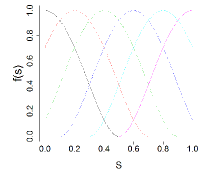
(a1)                                                      (a2)
                 
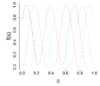
(b1)                                                      (b2)
                 
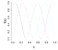
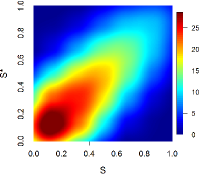
(c1)                                                      (c2)
                 
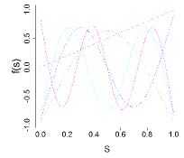
(d1)                                                      (d2)

Figure 1: (a1) Six basis functions corresponding to $\bm{f}^{(0)}(\cdot)$; (a2) The true spatial covariance function; (b1) Nine basis functions corresponding to $\bm{f}^{(1)}(\cdot)$; (b2) Spatial covariance function obtained from $\bm{f}^{(1)}(\cdot)$; (c1) Six basis functions corresponding to $\bm{f}^{(2)}(\cdot)$; (c2) Spatial covariance function obtained from $\bm{f}^{(2)}(\cdot)$; (d1) Six basis functions from the proposed method; (d2) Spatial covariance function obtained from the six proposed basis functions.

To further investigate the effect of $\bm{b}_{k}$’s and $r_{k}$’s in covariance function estimation, we consider two additional examples. For the first example, we apply the same basis functions of $\bm{f}^{(0)}(\bm{s})$ except that $r_{1}=\cdots=r_{6}=r\in[0.25,0.9]$. Figure 2 (a) shows how the ISE of (5) varies as a function of $r$. Not surprisingly, covariance function estimation is highly affected by $r$. For the second example, we consider the same bisque functions of (4) with $\bm{b}_{k}=0.2(k-1)+\Delta$; $k=1,\dots,7$ and $r_{1}=\cdots=r_{7}=0.5$, similar to those in Example 1. These can be regarded as shifted versions of $\bm{f}^{(0)}(\bm{s})$ controlled by a shift parameter $\Delta$. Figure 2 (b) shows the ISE of (5) with respect to $\Delta\in[-0.2,0]$. While ISE is less affected by $\Delta$ than $r$ in the first example, a poorly chosen $\Delta$ can still cause some significant bias in covariance function estimation.

(a)	(b)

Figure 2: (a) ISE values with respect to $r_{k}$ based on six basis functions of (4); (b) ISE values with respect to $\Delta$ with $\bm{b}_{k}=0.2(k-1)+\Delta$ based on seven basis functions of (4).

In this research, we propose a class of basis functions extracted from thin-plate splines. These functions are ordered in terms of their degrees of smoothness with a higher-order function corresponding to larger-scale features and a lower-order one corresponding to smaller-scale details, leading to a parsimonious representation for a nonstationary spatial covariance function. Consequently, only a small to moderate number of functions are needed in a spatial random-effects model. The proposed class of basis functions has several advantages over commonly used ones. First, we do not need to concern about the allocation of the basis functions, but simply select the total number of functions corresponding to a resolution. Second, only a small number of basis functions is usually required, which facilitates computation. Third, estimation variability of model parameters can be considerably reduced, and hence more precise covariance function estimates can be obtained. Fourth, the proposed basis functions depend only on the data locations but not the measurements taken at those locations, and are applicable regardless of whether the data locations are sparse or irregularly spaced.

The rest of the article is organized as follows. Section 2 introduces the proposed class of basis functions. In Section 3, we apply the proposed basis functions to spatial random-effects models, and derive simple close-form expressions for the maximum likelihood estimates of the model parameters. Some simulation examples and an application to a daily-temperature dataset in Canada are presented in Section 4.

2 The Proposed Ordered Set of Basis Functions

The proposed class of basis functions will be developed using thin-plate splines (TPSs). We shall first provide some basic knowledge about TPS. Given noisy data $\bm{Z}_{1},\dots,\bm{Z}_{n}$ observed at $n$ distinct control points, $\bm{s}_{1},\dots,\bm{s}_{n}\in\mathbb{R}^{d}$, a TPS function $f(\bm{s})$; $\bm{s}\in\mathbb{R}^{d}$, can be obtained by minimizing

$$\sum_{i=1}^{n}(Z_{i}-f(\bm{s}_{i}))^{2}+\rho J(f),$$ (6)

where $\bm{s}=(x_{1},\dots,x_{d})^{\prime}$,

$$J(f)=\int_{\mathbb{R}^{d}}\sum_{\nu_{1}+\cdots+\nu_{d}=2}\frac{2!}{\nu_{1}!\cdots\nu_{d}!}\left(\frac{\partial^{2}f(\bm{s})}{\partial x_{1}^{\nu_{1}}\cdots\partial x_{d}^{\nu_{d}}}\right)^{2}d\bm{s}\>\geq 0,$$ (7)

is a smoothness penalty, and $\rho\geq 0$ is a tuning parameter. It is known that (e.g., Wahba and Wendelberger, 1980; Green and Silverman, 1993) for $\rho>0$, the solution of (6) satisfies

$$f(\bm{s})=\bm{\alpha}^{\prime}\bm{\phi}(\bm{s})+\beta_{0}+\sum_{j=1}^{d}\beta_{j}x_{j}\textrm{ subject to }\bm{X}^{\prime}\bm{\alpha}=\bm{0},$$ (8)

where $\bm{s}_{i}=(x_{i1},\dots,x_{id})^{\prime}$; $i=1,\dots,n$,

$$\bm{X}=\left(\begin{matrix}1&x_{11}&\cdots&x_{1d}\\ \vdots&&\ddots&\\ 1&x_{n1}&\cdots&x_{nd}\end{matrix}\right),$$ (9)

and $\bm{\phi}(\bm{s})=(\phi_{1}(\bm{s}),\dots,\phi_{n}(\bm{s}))^{\prime}$ with

$$\phi_{i}(\bm{s})=\begin{cases}\displaystyle\frac{1}{12}\|\bm{s}-\bm{s}_{i}\|^{3};&\mathrm{if\>}d=1,\\ \displaystyle\frac{1}{8\pi}\|\bm{s}-\bm{s}_{i}\|^{2}\log\left(\|\bm{s}-\bm{s}_{j}\|\right);&\mathrm{if\>}d=2,\\ \displaystyle\frac{-1}{8}\|\bm{s}-\bm{s}_{i}\|;&\mathrm{if\>}d=3.\end{cases}$$ (10)

A function $f(\bm{s})$ in the form of (8) is called a natural TPS function. It has been shown that (e.g., Theorem 7.1 in Green and Silverman, 1993)

$$J(f)=\bm{\alpha}^{\prime}\bm{\Phi}\bm{\alpha},$$ (11)

where $\bm{\Phi}$ is the $n\times n$ matrix with the $(i,j)$-th element $\phi_{j}(\bm{s}_{i})$.

Assume that $\mathrm{rank}(\bm{X})=d+1$. We shall introduce our basis functions from the natural TPS function space:

$$\mathcal{F}=\Big{\{}f(\cdot):f(\bm{s})=\bm{\alpha}^{\prime}\bm{\phi}(\bm{s})+\beta_{0}+\sum_{j=1}^{d}\beta_{j}x_{j},\,\bm{\alpha}\in\mathbb{R}^{n},\bm{\beta}\in\mathbb{R}^{d+1},\,\bm{X}^{\prime}\bm{\alpha}=\bm{0}\Big{\}},$$ (12)

where $\bm{\beta}=(\beta_{0},\beta_{1},\dots,\beta_{d})^{\prime}$. The proposed basis functions form a basis of $\mathcal{F}$, and are defined as

$$f_{k}(\bm{s})=\begin{cases}1;&\quad k=1,\\ x_{k-1};&\quad k=2,\dots,d+1,\\ \lambda_{k-d-1}^{-1}\big{\{}\bm{\phi}(\bm{s})-\bm{\Phi}^{\prime}\bm{X}(\bm{X}^{\prime}\bm{X})^{-1}\bm{x}\big{\}}^{\prime}\bm{v}_{k-d-1}\big{\}};&\quad k=d+2,\dots,n,\end{cases}$$ (13)

where $\bm{x}=(1,\bm{s}^{\prime})^{\prime}=(1,x_{1},\dots,x_{d})^{\prime}$, $\bm{v}_{k}$ is the $k$-th column of $\bm{V}$, $\bm{V}\mathrm{diag}(\lambda_{1},\dots,\lambda_{n})\bm{V}^{\prime}$ is the eigen-decomposition of $\bm{Q\Phi Q}$ with $\lambda_{1}\geq\cdots\geq\lambda_{n}$, and $\bm{Q}=\bm{I}-\bm{X}(\bm{X}^{\prime}\bm{X})^{-1}\bm{X}^{\prime}$. Note that $\bm{\alpha}^{\prime}\bm{\Phi}\bm{\alpha}>0$ for all $\bm{\alpha}\neq\bm{0}$ with $\bm{X}^{\prime}\bm{\alpha}=\bm{0}$ (see Section 4 of Micchelli (1986)). Consequently, $\bm{a}^{\prime}\bm{Q}\bm{\Phi}\bm{Q}\bm{a}>0$ for all $\bm{a}$ satisfying $\bm{Q}\bm{a}\neq\bm{0}$, which implies $\mathrm{rank}(\bm{Q\Phi Q})=\mathrm{rank}(\bm{Q})=n-d-1$. Thus $\lambda_{1}\geq\cdots\geq\lambda_{n-d-1}>0$, and hence $f_{d+2}(\cdot),\dots,f_{n}(\cdot)$ are well defined.

The following theorem gives some important properties of these basis functions with its proof given in Appendix.

Theorem 1

Consider $f_{k}(\cdot)$’s in (13), $\mathcal{F}$ in (12), and $J(f)$ in (7), and assume that $\mathrm{rank}(\bm{X})=d+1<n$. Then

1. $\mathcal{F}=\Big{\{}\displaystyle\sum_{k=1}^{n}a_{k}f_{k}(\cdot):a_{k}\in\mathbb{R}\Big{\}}$.

2. $\{f_{1}(\cdot),\ldots,f_{d+1}(\cdot)\}$ is a basis of ${\displaystyle\left\{g(\cdot)\in\mathcal{F}:J(g)=0\right\}}.$

3. For $k=d+2,\dots,n$, define

   $$\mathcal{F}_{k}=\Big{\{}g(\cdot)\in\mathcal{F}:\sum_{i=1}^{n}g(\bm{s}_{i})^{2}=1,\,\sum_{i=1}^{n}g(\bm{s}_{i})f_{j}(\bm{s}_{i})=0;\,j=1,\dots,k-1\Big{\}}.$$ (14)

   Then $\displaystyle\mathop{\arg\min}_{g\in\mathcal{F}_{k}}J(g)=f_{k}(\cdot)$ and $J(f_{k})=\lambda_{k-d-1}^{-1}$, for $k=d+2,\dots,n$.

Remark 1

Let $\bm{f}_{k}=(f_{k}(\bm{s}_{1}),\dots,f_{k}(\bm{s}_{n}))^{\prime}$; $k=1,\dots,n$. Then $\bm{f}^{\prime}_{k}\bm{X}=\bm{0}$ and $\bm{f}^{\prime}_{k}\bm{f}_{k^{*}}=I(k=k^{*})$, for $k,k^{*}=d+2,\dots,n$.

Remark 2

The basis functions are given in a decreasing order in terms of their degrees of smoothness with $0=J(f_{1})=\cdots=J(f_{d+1})<J(f_{d+2})\leq\cdots\leq J(f_{n})$. In addition, $f_{k}(\cdot)$ is the smoothest function that is orthogonal to $f_{1}(\cdot),\dots,f_{k-1}(\cdot)$, for $k=d+2,\dots,n$. This enables a spatial process to be more parsimoniously represented in the spatial random-effects model, particularly when the underlying spatial covariance function is smooth. A one-dimensional example of $f_{2}(\cdot),\dots,f_{50}(\cdot)$ with $n=50$ and $s_{i}=i/50$; $i=1,\dots,50$, is shown in Figure 3.

Remark 3

Another basis of $\mathcal{F}$ is the Demmler-Reinsch basis (Demmler and Reinsch, 1975) given by

$$(h_{1}(\bm{s}),\dots,h_{n}(\bm{s}))^{\prime}=\bm{U}^{\prime}\big{(}(\bm{X},\bm{\Phi}\bm{N})^{\prime}(\bm{X},\bm{\Phi}\bm{N})\big{)}^{-1/2}\big{(}1,\bm{s}^{\prime},\bm{\phi}(\bm{s})^{\prime}\bm{N}\big{)}^{\prime},$$

where $\bm{N}$ is an $n\times(n-d-1)$ matrix such that $\bm{N}\bm{N}^{\prime}=\bm{Q}$ and $\bm{N}^{\prime}\bm{N}=\bm{I}_{n-d-1}$, and $\bm{U}\mathrm{diag}(a_{1},\dots,a_{n})\bm{U}^{\prime}$ is the eigen-decomposition of

$$\big{(}(\bm{X},\bm{\Phi}\bm{N})^{\prime}(\bm{X},\bm{\Phi}\bm{N})\big{)}^{-1/2}\left[\begin{array}[]{cc}\bm{0}&\bm{0}\\ \bm{0}&\bm{N}^{\prime}\bm{\Phi}\bm{N}\end{array}\right]\big{(}(\bm{X},\bm{\Phi}\bm{N})^{\prime}(\bm{X},\bm{\Phi}\bm{N})\big{)}^{-1/2},$$

with $a_{1}\geq\cdots\geq a_{n}$. While $h_{1}(\cdot),\dots,h_{n}(\cdot)$ are orthogonal and satisfy $J(h_{1})\leq\cdots\leq J(h_{n})$, they generally do not have the property of Theorem 1 (iii). Additionally, they are more expensive to compute since $\big{(}(\bm{X},\bm{\Phi}\bm{N})^{\prime}(\bm{X},\bm{\Phi}\bm{N})\big{)}^{-1/2}$ involves $O(n^{3})$ computations.

Figure 3: The proposed basis functions, $f_{2}(\cdot),\dots,f_{50}(\cdot)$.

Our method given by (13) requires computing only the first $K$ eigenvalue and eigenvector pairs of $\bm{Q}\bm{\Phi}\bm{Q}$ without the need to solve the full eigen-decomposition problem. In addition, we can compute $\bm{Q}\bm{\Phi}\bm{Q}=\tilde{\bm{Q}}-\tilde{\bm{X}}^{\prime}(\bm{X}^{\prime}\tilde{\bm{Q}})$ via $\tilde{\bm{X}}=(\bm{X}^{\prime}\bm{X})^{-1}\bm{X}^{\prime}$ and $\tilde{\bm{Q}}=\bm{\Phi}-(\bm{\Phi}\bm{X})\tilde{\bm{X}}$ to reduce the computations of $\bm{Q\Phi Q}$ from $O(n^{3})$ in terms of direct matrix multiplication to $O(n^{2}d)$. The first $K$ eigen-functions and eigenvalues can be efficiently obtained using some numerical techniques, such as the QR method and the Lanczos method (see e.g., Golub and van der Vorst, 2000; Ordonez et al. 2014) via an R package such as “bigpca” or “onlinePCA”. Both packages are available on Comprehensive R Archive Network (CRAN).

To know how the proposed basis functions perform in representing $C^{(0)}(\cdot,\cdot)$ of Example 1, we consider six basis functions $f_{1}(\cdot),\dots,f_{6}(\cdot)$ (see Figure 1 (d1)) derived from our method with the controlled points given at $s_{i}=i/50$; $i=1,\dots,50$, as in Figure 3. The best covariance function that minimizes (5) is shown in Figure 1 (d2). Clearly, it provides a much better approximation to the true spatial covariance function than those in Figure 1 (b2) and (c2) based on $\bm{f}^{(1)}(\cdot)$ and $\bm{f}^{(2)}(\cdot)$.

To illustrate how the proposed basis functions provide a multi-resolution covariance function representation, we consider a spatially deformed exponential covariance function:

$$C(s,s^{*})=\exp\big{\{}-2\big{|}(s+0.5)^{-1.5}-(s^{*}+0.5)^{-1.5}\big{|}\big{\}};\quad s,s^{*}\in[0,1]$$

(see Figure 4 (a)), which is a nonstationary covariance function constructed by applying a deformation transformation ($s\rightarrow(s+0.5)^{-1.5}$) to a stationary covariance function as in Sampson and Guttorp (1992). We apply our basis functions (see Figure 3) to approximate this covariance function, where the controlled points are given at $s_{i}=i/50$; $i=1,\dots,50$. The results for three different numbers of basis functions ($K=8,15,30$) are shown in Figure 4 (b)-(d), respectively. As you can see, large-scale features can be captured even if $K$ is merely $8$. On the other hand, finer-resolution details are captured by $f_{k}(\cdot)$ with larger $k$ values.

(a)	(b)
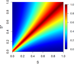
(c)	(d)

Figure 4: (a) A nonstationary spatial covariance function; (b) covariance function approximation based on $8$ basis functions; (c) covariance function approximation based on $15$ basis functions; (d) covariance function approximation based on $30$ basis functions.

The proposed class of basis functions is even more effective in the two-dimensional space. Suppose that we would like to approximate an exponential covariance function, $C(\bm{s},\bm{s}^{*})=20\exp(-0.4\|\bm{s}-\bm{s}^{*}\|)$ for $\bm{s},\bm{s}^{*}\in[0,1]^{2}$, using $\bm{f}(\bm{s})^{\prime}\bm{M}\bm{f}(\bm{s})$. We compare between a conventional method and our method. For a conventional method, we consider the natural TPS functions for $\bm{f}(\cdot)$ formed by $1$, $x_{1}$, $x_{2}$ and

$$\frac{1}{8\pi}\bigg{\|}\bm{s}-\bigg{(}\frac{\ell_{1}}{L+1},\frac{\ell_{2}}{L+1}\bigg{)}^{\prime}\bigg{\|}^{2}\log\bigg{\{}\bigg{\|}\bm{s}-\bigg{(}\frac{\ell_{1}}{L+1},\frac{\ell_{2}}{L+1}\bigg{)}^{\prime}\bigg{\|}\bigg{\}};\quad 1\leq\ell_{1},\ell_{2}\leq L,$$

with their centers regularly location in $[0,1]^{2}$ for $L\in\{3,5,7,9,11,13\}$, corresponding to a total of $\{12,28,52,84,124,172\}$ basis functions. We apply our method with the control points, $\{((2j_{1}-1)/36,(2j_{2}-1)/36):1\leq j_{1},j_{2}\leq 18\}$, regularly located in $[0,1]^{2}$, and consider the same numbers of basis functions for comparison. The performance between the conventional basis functions and the proposed basis functions is shown in Table 1. For all cases, the proposed basis functions provide much better approximation ability than the conventional basis functions.

Table 1: ISE performance between TPS basis functions and the proposed basis functions for various numbers of functions.

number of basis functions	TPS	Proposed
$3^{2}$+3	0.09462	0.01895
$5^{2}$+3	0.01505	0.00301
$7^{2}$+3	0.00416	0.00085
$9^{2}$+3	0.00155	0.00037
$11^{2}$+3	0.00070	0.00021
$13^{2}$+3	0.00037	0.00015

3 Parameter Estimation

Consider the spatial random-effects model given by (1) and (2). For simplicity, we assume that $\mu(\bm{s},t)=0$ and $\sigma_{\epsilon}^{2}$ is known, since $\sigma_{\epsilon}^{2}$ and $\sigma_{\xi}^{2}$ are confounded together unless some additional information is available. Given the basis functions $f_{1}(\cdot),\dots,f_{K}(\cdot)$, the parameters that need to be estimated are $\bm{M}$, which has to be non-negative definite, and $\sigma_{\xi}^{2}\geq 0$. Although the ML estimates $\hat{\bm{M}}_{K}$ and $\hat{\sigma}_{\xi,K}^{2}$ of $\bm{M}$ and $\sigma_{\xi}^{2}$ can be computed using the EM algorithm (Katzfuss and Cressie, 2009), as shown in the following theorem, a closed-form expression for $\hat{\bm{M}}_{K}$ can be derived with its proof given in Appendix. The estimate $\hat{\sigma}_{\xi,K}^{2}$ can be computed using a simple one-dimensional optimization method.

Theorem 2

Consider the model given by (1) and (2) with $\mu(\bm{s},t)=0$ and $\sigma_{\epsilon}^{2}$ known. Then the ML estimates of $\bm{M}$ and $\sigma_{\xi}^{2}$ are given by

$$\hat{\sigma}_{\xi,K}^{2}= \leavevmode\nobreak\ \mathop{\arg\min}_{\sigma_{\xi}^{2}}\left[\frac{\mathrm{tr}(\bm{S})}{\sigma_{\xi}^{2}+\sigma_{\epsilon}^{2}}+\sum_{k=1}^{K}\bigg{\{}\log\big{(}\hat{d}_{K,k}+\sigma_{\xi}^{2}+\sigma_{\epsilon}^{2}\big{)}-\frac{d_{K,k}\hat{d}_{K,k}}{\sigma_{\xi}^{2}+\sigma_{\epsilon}^{2}}\bigg{\}}+(n-K)\log(\sigma_{\xi}^{2}+\sigma_{\epsilon}^{2})\right],$$

$$\hat{\bm{M}}_{K}= \leavevmode\nobreak\ \left(\bm{F}^{\prime}_{K}\bm{F}_{K}\right)^{-1/2}\bm{P}_{K}\,\mathrm{diag}\big{(}\hat{d}_{K,1},\dots,\hat{d}_{K,K}\big{)}\bm{P}^{\prime}_{K}\left(\bm{F}^{\prime}_{K}\bm{F}_{K}\right)^{-1},$$

where $\bm{S}=\displaystyle\sum_{t=1}^{T}\bm{z}_{t}\bm{z}^{\prime}_{t}/T$, $\bm{F}_{K}=(\bm{f}_{1},\dots,\bm{f}_{K})$, $\bm{f}_{k}=(f_{k}(\bm{s}_{1}),\dots,f_{k}(\bm{s}_{n}))^{\prime}$; $k=1,\dots,K$, $\bm{P}_{K}\,\mathrm{diag}(d_{K,1},\dots,d_{K,K})\bm{P}^{\prime}_{K}$ is the eigen-decomposition of $(\bm{F}^{\prime}_{K}\bm{F}_{K})^{-1/2}\bm{F}^{\prime}_{K}\bm{S}\bm{F}_{K}\left(\bm{F}^{\prime}_{K}\bm{F}_{K}\right)^{-1/2}$, and $\hat{d}_{K,k}=\max\left(d_{K,k}-\hat{\sigma}_{\xi,K}^{2}-\sigma_{\epsilon}^{2},0\right)$; $k=1,\dots,K$.

In practice, we propose to select $K\in\{d+1,\dots,K^{*}\}$ for a sufficiently large $K^{*}$ using Akaike’s information criterion (AIC, Akaike, 1973, 1974):

$$\mathrm{AIC}(K)= \leavevmode\nobreak\ T\log\big{|}\hat{\bm{\Sigma}}_{k}\big{|}+T\mathrm{tr}\big{(}\bm{S}\hat{\bm{\Sigma}}^{-1}_{K}\big{)}+K^{2}+K+2$$

$$= \leavevmode\nobreak\ \frac{T\mathrm{tr}(\bm{S})}{\hat{\sigma}_{\xi,K}^{2}+\sigma_{\epsilon}^{2}}+T\sum_{k=1}^{K}\bigg{\{}\log\big{(}\hat{d}_{K,k}+\hat{\sigma}_{\xi,K}^{2}+\sigma_{\epsilon}^{2}\big{)}-\frac{d_{K,k}\hat{d}_{K,k}}{\hat{\sigma}_{\xi,K}^{2}+\sigma_{\epsilon}^{2}}\bigg{\}}+K^{2}+K+2,$$

where $\hat{\bm{\Sigma}}_{K}=\bm{F}_{K}\hat{\bm{M}}_{K}\bm{F}^{\prime}_{K}+(\hat{\sigma}_{\xi,K}^{2}+\sigma_{\epsilon}^{2})\bm{I}_{n}$. Then the final number of basis functions selected by AIC is $\hat{K}=\displaystyle\mathop{\arg\min}_{d+1\leq K\leq K^{*}}\mathrm{AIC}(K)$. Plugging in $\hat{\bm{M}}_{\hat{K}}$ and $\hat{\sigma}_{\xi,\hat{K}}^{2}$ into the best linear unbiased predictor of $y(\bm{s},t)$, we obtain

$$\hat{y}(\bm{s},t)=\big{\{}\bm{f}(\bm{s})^{\prime}\bm{\hat{M}}_{\hat{K}}\bm{F}^{\prime}_{K}+\hat{\sigma}_{\xi,\hat{K}}^{2}(I(\bm{s}=\bm{s}_{1}),\dots,I(\bm{s}=\bm{s}_{n}))\big{\}}\bm{\hat{\Sigma}}^{-}_{\hat{K}}\bm{z}_{t}\>;\quad\bm{s}\in D,\,t=1,\dots,T,$$ (15)

where $\bm{\hat{\Sigma}}^{-}_{\hat{K}}$ is the Moore-Penrose inverse of $\bm{\hat{\Sigma}}_{\hat{K}}$ and can be efficiently computed by

$$\begin{cases}\displaystyle\frac{1}{\hat{\sigma}_{\xi,\hat{K}}^{2}+\sigma_{\epsilon}^{2}}\left\{\bm{I}_{n}-\bm{L}_{\hat{K}}\bm{P}_{\hat{K}}\,\mathrm{diag}\bigg{(}\frac{d_{\hat{K},1}}{d_{\hat{K},1}+\hat{\sigma}_{\xi,\hat{K}}^{2}+\sigma_{\epsilon}^{2}},\dots,\frac{d_{\hat{K},\hat{K}}}{d_{\hat{K},\hat{K}}+\hat{\sigma}_{\xi,\hat{K}}^{2}+\sigma_{\epsilon}^{2}}\bigg{)}\bm{P}^{\prime}_{\hat{K}}\bm{L}^{\prime}_{\hat{K}}\right\};&\mathrm{if}\leavevmode\nobreak\ \hat{\sigma}_{\xi,\hat{K}}^{2}+\sigma_{\epsilon}^{2}>0,\\ \bm{L}_{\hat{K}}\bm{P}_{\hat{K}}\,\big{\{}\mathrm{diag}\big{(}d_{\hat{K},1},\dots,d_{\hat{K},\hat{K}}\big{)}\big{\}}^{-}\bm{P}^{\prime}_{\hat{K}}\bm{L}^{\prime}_{\hat{K}};&\mathrm{if}\leavevmode\nobreak\ \hat{\sigma}_{\xi,\hat{K}}^{2}=\sigma_{\epsilon}^{2}=0,\end{cases}$$ (16)

and $\bm{L}_{\hat{K}}=\bm{F}_{\hat{K}}(\bm{F}^{\prime}_{\hat{K}}\bm{F}_{\hat{K}})^{-1/2}$.

4 Numeric Examples

4.1 Simulation

In the simulation, we considered spatial processes, $\{y(\bm{s},t):\bm{s}\in[0,1]^{2}\}$ for $t=1,\dots,50$, generated from (2) with $\mu(\bm{s},t)=0$, $f_{1}(\bm{s})=\cos(\pi\|\bm{s}-(0,1)^{\prime}\|)$, $f_{2}(\bm{s})=\cos(2\pi\|\bm{s}-(3/4,1/4)^{\prime}\|)$, and $(w_{1}(t),w_{2}(t))^{\prime}\sim N(\bm{0},\mathrm{diag}(25,9))$, where $f_{1}(\cdot)$ and $f_{2}(\cdot)$ are shown in Figure 5. We generated data, $\bm{z}_{1},\dots,\bm{z}_{50}$, according to (1) with $n=100$ and $\sigma_{\epsilon}^{2}=3$, where $\bm{s}_{1},\dots,\bm{s}_{n}$ were taken from $D=[0,1]^{2}$ using simple random sampling.

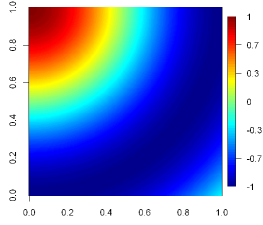
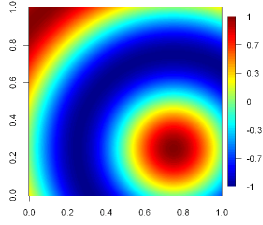
(a)	(b)

Figure 5: Basis functions in a spatial random-effects model: (a) $f_{1}(\cdot)$; (b) $f_{2}(\cdot)$.

We applied the spatial random-effects model of (1) and (2) and the ML estimates given by Theorem 2 to estimate the underlying spatial covariance function with $\sigma_{\epsilon}^{2}=3$ assumed known. We considered commonly used bisquare basis functions given in (4) with six different layouts for function centers and radii at two resolutions (see Table 2). We applied the proposed basis functions and selected the number of basis functions among $K\in\{3,\dots,20\}$ using AIC. We also considered the exponential covariance model and the true covariance function for comparison. All the model parameters were estimated by ML.

Table 2: Various layouts for centers of the bisque basis functions.

Layout	Coarse Resolution		Fine Resolution		K
	Center	Radius	Center	Radius
1	$\{0,1\}^{2}$	$3/2$	$\{1/4,3/4\}^{2}$	$3/4$	$8$
2	$\{1/6,5/6\}^{2}$	$1$	$\{0,1/2,1\}^{2}$	$3/2$	$13$
3	$\{1/6,5/6\}^{2}\cup(1/2,1/2)$	$\sqrt{2}/2$	$\{0,1/2,1\}^{2}$	$3/2$	$14$
4	$\{0,1/2,1\}^{2}$	$3/4$	$\{1/6,1/2,5/6\}^{2}$	$1/2$	$18$
5	$\{1/6,5/6\}^{2}$	$1$	$\{0,1/3,2/3,1\}^{2}$	$1/2$	$20$
6	$\{1/6,5/6\}^{2}\cup(1/2,1/2)$	$\sqrt{2}/2$	$\{0,1/3,2/3,1\}^{2}$	$1/2$	$21$

The performance of various methods was compared in terms of the mean-squared-prediction-error (MSPE) criterion:

$$\frac{1}{50}\sum_{t=1}^{50}\int_{[0,1]^{2}}E(\hat{y}(\bm{s},t)-y(\bm{s},t))^{2},$$

where $\hat{y}(\bm{s},t)$ is a generic predictor of $y(\bm{s},t)$ obtained from simple kriging based on $\bm{z}_{t}$ using an (estimated) spatial covariance model. The results based on 200 simulation replicates are shown in Table 3. Not surprisingly, bisquare basis functions perform well for some cases but poorly for others. In contrast, our method performs better than all the other spatial covariance estimation methods by having a smaller averaged MSPE value. The first and the third quantiles for the distribution of the number of basis functions selected by AIC are about 10 and 12, indicating that only a small number of basis functions is required.

Table 3: Averaged MSPEs for various methods based on 200 simulation replicates. Values given in parentheses are the corresponding standard errors.

True	Exponential	Our	Bisque Basis Functions
			1	2	3	4	5	6
0.123	1.234	0.646	0.694	0.872	1.063	0.962	1.013	1.191
(0.015)	(0.017)	(0.015)	(0.024)	(0.018)	(0.031)	(0.034)	(0.032)	(0.037)

4.2 Application to Canadian Temperature Data

We applied the proposed method to an average daily temperature dataset. The data, available in the “fda” package on CRAN, consist of average temperatures for each day of the year at 35 weather stations in Canada, which are averaged over years 1960 to 1994. They have been analyzed by Ramsay and Dalzell (1991) and Silverman and Ramsay (2005) using functional data analysis techniques without considering spatial dependence.

Let $z(\bm{s}_{i},t)$ be the average daily temperature at location $\bm{s}_{i}$ and day $t$, where $\bm{s}_{i}$ is given with coordinates in latitude and longitude in units of degrees. We considered the spatial random-effects model of (1) and (2) with $n=35$ and $T=365$. Since the temporal patterns are known to be different at different stations (see e.g., Silverman, 1995), we considered a semiparametric model (Buja et al., 1989) for $\mu(\bm{s},t)$ with station-specific quadratic effects:

$$\mu(\bm{s},t)=m_{0}(t)+m(\bm{s})+\ell(\bm{s})t+q(\bm{s})t^{2};\quad\bm{s}\in D,\,t=1,\dots,365,$$ (17)

where $m_{0}(\cdot),m(\cdot),\ell(\cdot)$ and $q(\cdot)$ are unknown smooth functions, and for identification purpose, we assume $\displaystyle\sum_{i=1}^{35}m(\bm{s}_{i})=\displaystyle\sum_{i=1}^{35}\ell(\bm{s}_{i})=\displaystyle\sum_{i=1}^{35}q(\bm{s}_{i})=0$.

We considered a two-step procedure to fit $\mu(\cdot,\cdot)$ with the smoothness parameter selected by using Mallow’s $C_{p}$ (Hastie and Tibshirani, 1990). First, we obtained the estimates $\hat{m}_{i}$, $\hat{\ell}_{i}$ and $\hat{q}_{i}$ of $m(\bm{s}_{i})$, $\ell(\bm{s}_{i})$ and $q(\bm{s}_{i})$ for $i=1,\dots,35$, and the estimate $\hat{m}_{0}(\cdot)$ of $m_{0}(\cdot)$ using the R package “gam” available on CRAN (see Figure 6 (a)). Then we separately applied smoothing splines to $\hat{m}_{i}$’s, $\hat{\ell}_{i}$’s and $\hat{q}_{i}$’s and obtained the estimates $\hat{m}_{i}(\cdot)$, $\hat{\ell}(\cdot)$ and $\hat{q}(\cdot)$ (see Figure 6 (b)-(d)) with the smoothing parameter selected by generalized cross-validation (Golub et al., 1979). Then we assume that $\mu(\bm{s},t)$ is known as $\hat{\mu}(\bm{s},t)=\hat{m}_{0}(t)+\hat{m}(\bm{s})+\hat{\ell}(\bm{s})t+\hat{q}(\bm{s})t^{2}$ for covariance function estimation.

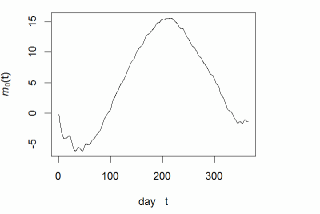
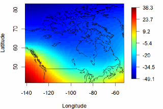
(a)	(b)
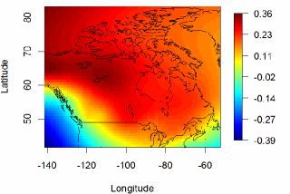
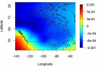
(c)	(d)

Figure 6: Estimated functions in (17): (a) $\hat{m}_{0}(t)$; (b) $\hat{m}(\bm{s})$; (c) $\hat{\ell}(\bm{s})$; (d) $\hat{q}(\bm{s})$.

We randomly divided the data into two parts with one part consisting of 185 time points as the training data, and the other part consisting of 180 time points as the testing data. We applied the spatial random-effects model of (1) and (2). We assumed that $\sigma_{\xi}^{2}=0$, but $\sigma_{\epsilon}^{2}$ is unknown, and applied ML with the proposed basis functions to estimate the underlying spatial covariance function. We also considered applying the exponential covariance model to estimate covariance function with the parameters estimated by ML.

The performance of the two covariance function estimates is evaluated in terms of the Frobenius loss, $\mathrm{Loss}_{F}=\|\hat{\bm{\Sigma}}-\bm{S}_{\mathrm{test}}\|$ and the Kullbeck-Leibler loss, $\mathrm{Loss}_{KL}=\frac{1}{2}\big{\{}\mathrm{tr}(\hat{\bm{\Sigma}}^{-1}\bm{S}_{\mathrm{test}})+\log|\hat{\bm{\Sigma}}|-\log|\bm{S}_{\mathrm{test}}|-35\big{\}}$, where $\bm{\hat{\Sigma}}$ is a generic estimate of $\bm{\Sigma}$ and $\bm{S}_{\mathrm{test}}$ is the sample covariance matrix based on the testing data. The validation procedure was repeated 100 times. The average $\mathrm{Loss}_{F}$ and $\mathrm{Loss}_{KL}$ based on our method are $10.0$ and $4.7$ respectively, which are much smaller than $177.1$ and $25.7$ based on the exponential covariance model, which is not surprising, because the data are highly nonstationary in space. The mean surfaces $\mu(\cdot,t)$ and the final predicted surfaces $\hat{y}(\cdot,t)$ of $y(\cdot,t)$ for $t=50,125,200$ are shown in Figure 7.

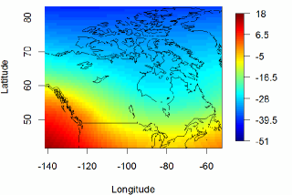
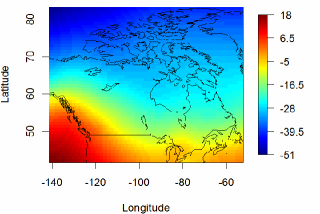
(a1)	(a2)
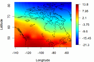
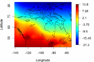
(b1)	(b2)
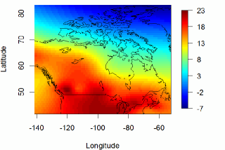
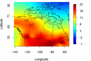
(c1)	(c2)

Figure 7: (a1) $\mu(\bm{s},50)$; (a2) $\hat{y}(\bm{s},50)$; (b1) $\mu(\bm{s},125)$; (b2) $\hat{y}(\bm{s},125)$; (c1) $\mu(\bm{s},200)$; (c2) $\hat{y}(\bm{s},200)$.

Appendix

Proof of Theorem 1

(i) We first show that $\displaystyle\sum_{k=1}^{n}a_{k}f_{k}(\cdot)\in\mathcal{F}$, for any given $a_{1},\dots,a_{n}\in\mathbb{R}$. Direct calculation gives

$$\sum_{k=1}^{n}a_{k}f_{k}(\cdot)=\bm{\alpha}^{\prime}\bm{\phi}(\bm{s})+\bm{\beta}^{\prime}(1,x_{1},\dots,x_{d})^{\prime},$$

where

$$\bm{\alpha}= \leavevmode\nobreak\ \bm{V}_{n-d-1}\mathrm{diag}(\lambda_{1}^{-1},\dots,\lambda_{n-d-1}^{-1})(a_{d+2},\dots,a_{n})^{\prime},$$ (18)

$$\bm{\beta}= \leavevmode\nobreak\ (a_{1},\ldots,a_{d+1})^{\prime}-(\bm{X}^{\prime}\bm{X})^{-1}\bm{X}^{\prime}\bm{\Phi}\bm{V}_{n-d-1}\mathrm{diag}(\lambda_{1}^{-1},\dots,\lambda_{n-d-1}^{-1})(a_{d+2},\dots,a_{n})^{\prime},$$

and $\bm{V}_{n-d-1}$ is the submatrix of $\bm{V}$ in (13) consisting of its first $n-d-1$ columns. By the definition of $\bm{V}$, $\bm{Q}\bm{\Phi}\bm{Q}=\bm{V}_{n-d-1}\mathrm{diag}(\lambda_{1},\ldots,\lambda_{n-d-1})\bm{V}_{n-d-1}^{\prime}$, and hence

$$\bm{V}_{n-d-1}=\bm{Q}\bm{\Phi}\bm{Q}\bm{V}_{n-d-1}\mathrm{diag}(\lambda_{1}^{-1},\ldots,\lambda_{n-d-1}^{-1}).$$ (19)

This together with (18) and $\bm{X}^{\prime}\bm{Q}=\bm{0}$ implies that $\bm{X}^{\prime}\bm{\alpha}=\bm{0}$. Thus $\displaystyle\sum_{k=1}^{n}a_{k}f_{k}(\cdot)\in\mathcal{F}$ is proved.

We remain to show that $\mathcal{F}\subset\Big{\{}\displaystyle\sum_{k=1}^{n}a_{k}f_{k}(\cdot):a_{k}\in\mathbb{R}\Big{\}}$. We first show that

$$\bm{V}_{n-d-1}\bm{V}_{n-d-1}^{\prime}=\bm{Q}.$$ (20)

From (19) and $\bm{X}^{\prime}\bm{Q}=\bm{0}$, we have $\bm{X}\bm{V}_{n-d-1}\bm{V}_{n-d-1}^{\prime}=\bm{0}$. This and the fact that $\bm{V}_{n-d-1}\bm{V}_{n-d-1}^{\prime}$ is idempotent of rank $n-d-1$ imply that $\bm{V}_{n-d-1}\bm{V}_{n-d-1}^{\prime}$ is the projection matrix for the space orthogonal to the column space of $\bm{X}$. That is, $\bm{V}_{n-d-1}\bm{V}_{n-d-1}^{\prime}=\bm{Q}$.

Given any $f(\bm{s})=\bm{\alpha}^{\prime}\bm{\phi}(\bm{s})+\beta_{0}+\displaystyle\sum_{j=1}^{d}\beta_{j}x_{j}\in\mathcal{F}$, since $\bm{X}^{\prime}\bm{\alpha}=\bm{0}$, we can write

$$f(\bm{s})= \leavevmode\nobreak\ \bm{\phi}(\bm{s})^{\prime}(\bm{\alpha}-\bm{X}(\bm{X}^{\prime}\bm{X})^{-1}\bm{X}^{\prime}\bm{\alpha})+(1,x_{1},\dots,x_{d})^{\prime}\bm{\beta}$$

$$= \leavevmode\nobreak\ (\bm{\phi}(\bm{s})^{\prime},1,x_{1},\dots,x_{d})\begin{bmatrix}\bm{V}_{n-d-1}\bm{V}_{n-d-1}^{\prime}&\bm{0}\\ \bm{0}&\bm{I}_{d+1}\end{bmatrix}\begin{bmatrix}\bm{\alpha}\\ \bm{\beta}\end{bmatrix}$$

$$= \leavevmode\nobreak\ (\bm{\phi}(\bm{s})^{\prime},1,x_{1},\ldots,x_{d})\begin{bmatrix}\bm{0}&\bm{V}_{n-d-1}\mathrm{diag}(\lambda_{1}^{-1},\ldots,\lambda_{n-d-1}^{-1})\\ \bm{I}_{d+1}&-(\bm{X}^{\prime}\bm{X})^{-1}\bm{X}^{\prime}\bm{\Phi}\bm{V}_{n-d-1}\mathrm{diag}(\lambda_{1}^{-1},\ldots,\lambda_{n-d-1}^{-1})\end{bmatrix}$$

$$\leavevmode\nobreak\ \times\begin{bmatrix}(\bm{X}^{\prime}\bm{X})^{-1}\bm{X}^{\prime}\bm{\Phi}\bm{V}_{n-d-1}\bm{V}_{n-d-1}^{\prime}&\bm{I}_{d+1}\\ \mathrm{diag}(\lambda_{1},\ldots,\lambda_{n-d-1})\bm{V}_{n-d-1}^{\prime}&\bm{0}\end{bmatrix}\begin{bmatrix}\bm{\alpha}\\ \bm{\beta}\end{bmatrix}$$

$$= \leavevmode\nobreak\ (f_{1}(\bm{s}),\ldots,f_{n}(\bm{s}))\begin{bmatrix}(\bm{X}^{\prime}\bm{X})^{-1}\bm{X}^{\prime}\bm{\Phi}\bm{V}_{n-d-1}\bm{V}_{n-d-1}^{\prime}\bm{\alpha}+\bm{\beta}\\ \mathrm{diag}(\lambda_{1},\ldots,\lambda_{n-d-1})\bm{V}_{n-d-1}^{\prime}\bm{\alpha}\end{bmatrix},$$

where the second equality follows from (20). Thus $f(\cdot)\in\Big{\{}\displaystyle\sum_{k=1}^{n}a_{k}f_{k}(\cdot):a_{k}\in\mathbb{R}\Big{\}}$. This completes the proof of (i).

(ii) Clearly, $J(f_{1})=\cdots=J(f_{d+1})=0$. It suffices to show that $J(f)=\bm{\alpha}^{\prime}\bm{\Phi}\bm{\alpha}>0$ for any $f(\bm{s})=\bm{\alpha}^{\prime}\bm{\phi}(\bm{s})+\beta_{0}+\displaystyle\sum_{j=1}^{d}\beta_{j}x_{j}\in\mathcal{F}$ with $\bm{\alpha}\neq\bm{0}$. Since $\mathrm{rank}(\bm{X})=d+1$, $\bm{X}^{\prime}\bm{\alpha}=\bm{0}$ and $\bm{\alpha}\neq\bm{0}$, it follows that $\bm{\alpha}^{\prime}\bm{\Phi}\bm{\alpha}>0$ (see Section 4 of Micchelli (1986)). This completes the proof of (ii).

(iii) We shall only prove the result for $k=d+2$. Given any $g(\cdot)\in\mathcal{F}$, let $\bm{g}=(g(\bm{s}_{1}),\dots,g(\bm{s}_{n}))^{\prime}=\bm{\Phi}\bm{\alpha}_{g}+\bm{X}\bm{\beta}_{g}$. Then $g(\cdot)\in\mathcal{F}_{d+2}$ if and only if

$$(\bm{\alpha}_{g},\bm{\beta}_{g})\in \leavevmode\nobreak\ \big{\{}(\bm{\alpha},\bm{\beta}):\bm{X}^{\prime}\bm{\alpha}=0,\,\bm{X}^{\prime}\bm{g}=\bm{0},\mbox{ and }\|\bm{g}\|_{2}=1\big{\}}$$

$$= \leavevmode\nobreak\ \big{\{}(\bm{\alpha},\bm{\beta}):\bm{X}^{\prime}\bm{\alpha}=0,\,\bm{g}=\bm{Q}\bm{g}=\bm{Q}\bm{\Phi}\bm{\alpha},\mbox{ and }\|\bm{g}\|_{2}=1\big{\}}$$

$$= \leavevmode\nobreak\ \big{\{}(\bm{\alpha},\bm{\beta}):\bm{\alpha}=\bm{Q}\bm{\alpha},\,\bm{\beta}=-(\bm{X}^{\prime}\bm{X})^{-1}\bm{X}^{\prime}\bm{\Phi}\bm{\alpha},\mbox{ and }\|\bm{Q}\bm{\Phi}\bm{Q}\bm{\alpha}\|_{2}=1\big{\}}.$$ (21)

Therefore, from (11) and (21),

$$\min_{g(\cdot)\in\mathcal{F}_{d+2}}J(g)= \leavevmode\nobreak\ \min\{\bm{\alpha}^{\prime}\bm{\Phi}\bm{\alpha}:\bm{\alpha}\in\mathbb{R}^{n},\,\bm{\alpha}=\bm{Q}\bm{\alpha},\,\|\bm{Q}\bm{\Phi}\bm{Q}\bm{\alpha}\|_{2}=1\}$$

$$= \leavevmode\nobreak\ \min\{\bm{\alpha}^{\prime}\bm{Q}\bm{\Phi}\bm{Q}\bm{\alpha}:\bm{\alpha}\in\mathbb{R}^{n},\,\|\bm{Q}\bm{\Phi}\bm{Q}\bm{\alpha}\|_{2}=1\}$$

$$= \leavevmode\nobreak\ \min\{\bm{\alpha}^{\prime}\bm{V}\bm{\Lambda}\bm{V}^{\prime}\bm{\alpha}:\bm{\alpha}\in\mathbb{R}^{n},\,\|\bm{\Lambda}\bm{V}^{\prime}\bm{\alpha}\|_{2}=1\}$$

$$= \leavevmode\nobreak\ \min\{\bm{a}^{\prime}\bm{\Lambda}\bm{a}:\bm{a}\in\mathbb{R}^{n},\,\|\bm{\Lambda}\bm{a}\|_{2}=1\}=\lambda_{1}^{-1},$$ (22)

where $\bm{\Lambda}=\mathrm{diag}(\lambda_{1},\dots,\lambda_{n})$. It follows from (21) and (22) that

$$\big{(}\lambda_{1}^{-1}\bm{v}_{1},\,-\lambda_{1}^{-1}(\bm{X}^{\prime}\bm{X})^{-1}\bm{X}^{\prime}\bm{\Phi}\bm{v}_{1}\big{)}=\mathop{\arg\min}_{(\bm{\alpha},\bm{\beta})}\big{\{}J(g):g(\bm{x})=\bm{\phi}(\bm{x})^{\prime}\bm{\alpha}+(1,x_{2},\dots,x_{d})^{\prime}\bm{\beta}\in\mathcal{F}_{d+2}\big{\}}.$$

This proves (iii) and the proof of Theorem 2 is complete.

Proof of Theorem 2

Let $\bm{H}=\bm{F}_{K}(\bm{F}^{\prime}_{K}\bm{F}_{K})^{-1}\bm{F}^{\prime}_{K}$, $\bm{L}_{K}=\bm{F}_{K}(\bm{F}^{\prime}_{K}\bm{F}_{K})^{-1/2}$, and $\bm{R}=\bm{L}_{K}\bm{P}_{K}$. It follows from the definition of $\bm{P}_{K}\mathrm{diag}(d_{K,1},\dots,d_{K,K})\bm{P}^{\prime}_{K}$ and simple algebra that $\bm{H}\bm{S}\bm{H}=\bm{R}\,\mathrm{diag}(d_{K,1},\dots,d_{K,K})\bm{R}^{\prime}$. Since $\mathrm{rank}(\bm{F}_{K}\bm{M}\bm{F}^{\prime}_{K})\leq K$, the eigen-decomposition of $\bm{F}_{K}\bm{M}\bm{F}^{\prime}_{K}$ can be written as $\tilde{\bm{R}}\,\mathrm{diag}(\tilde{d}_{1},\dots,\tilde{d}_{K})\tilde{\bm{R}}^{\prime}$, where $\tilde{\bm{R}}$ is an $n\times K$ matrix with orthonormal columns. Using $\bm{H}\bm{F}_{K}=\bm{F}_{K}$, we have

$$\{\bm{F}_{K}\bm{M} \bm{F}^{\prime}_{K}+(\sigma_{\xi}^{2}+\sigma_{\epsilon}^{2})\bm{I}_{n}\}^{-1}$$

$$= \leavevmode\nobreak\ \big{\{}\bm{H}\tilde{\bm{R}}\,\mathrm{diag}\big{(}\tilde{d}_{1},\dots,\tilde{d}_{K}\big{)}\tilde{\bm{R}}^{\prime}\bm{H}+(\sigma_{\xi}^{2}+\sigma_{\epsilon}^{2})\bm{I}_{n}\big{\}}^{-1}$$

$$= \leavevmode\nobreak\ \frac{1}{\sigma_{\xi}^{2}+\sigma_{\epsilon}^{2}}\bm{I}_{n}-\frac{1}{\sigma_{\xi}^{2}+\sigma_{\epsilon}^{2}}\bm{H}\tilde{\bm{R}}\,\mathrm{diag}\bigg{(}\frac{\tilde{d}_{1}}{\tilde{d}_{1}+\sigma_{\xi}^{2}+\sigma_{\epsilon}^{2}},\dots,\frac{\tilde{d}_{K}}{\tilde{d}_{K}+\sigma_{\xi}^{2}+\sigma_{\epsilon}^{2}}\bigg{)}\tilde{\bm{R}}^{\prime}\bm{H}.$$

Then twice the negative log-likelihood function of $\bm{z}_{1},\dots,\bm{z}_{T}$ is

$$\ell(\bm{M}, \sigma_{\xi}^{2})=nT\log 2\pi+\log\big{|}\bm{F}_{K}\bm{M}\bm{F}^{\prime}_{K}+(\sigma_{\xi}^{2}+\sigma_{\epsilon}^{2})\bm{I}_{n}\big{|}+\mathrm{tr}\big{\{}\bm{S}(\bm{F}_{K}\bm{M}\bm{F}^{\prime}_{K}+(\sigma_{\xi}^{2}+\sigma_{\epsilon}^{2})\bm{I}_{n}\big{)}^{-1}\big{\}}$$

$$= \leavevmode\nobreak\ nT\log 2\pi+\log\big{|}\tilde{\bm{R}}\,\mathrm{diag}\big{(}\tilde{d}_{1},\dots,\tilde{d}_{K}\big{)}\tilde{\bm{R}}^{\prime}+(\sigma_{\xi}^{2}+\sigma_{\epsilon}^{2})\bm{I}_{n}\big{|}$$

$$\leavevmode\nobreak\ +\mathrm{tr}\bigg{(}\frac{1}{\sigma_{\xi}^{2}+\sigma_{\epsilon}^{2}}\bm{S}-\frac{1}{\sigma_{\xi}^{2}+\sigma_{\epsilon}^{2}}\bm{S}\bm{H}\tilde{\bm{R}}\,\mathrm{diag}\bigg{(}\frac{\tilde{d}_{1}}{\tilde{d}_{1}+\sigma_{\xi}^{2}+\sigma_{\epsilon}^{2}},\dots,\frac{\tilde{d}_{K}}{\tilde{d}_{K}+\sigma_{\xi}^{2}+\sigma_{\epsilon}^{2}}\bigg{)}\tilde{\bm{R}}^{\prime}\bm{H}\bigg{)}$$

$$= \leavevmode\nobreak\ nT\log 2\pi+\bigg{\{}\sum_{k=1}^{K}\log\big{(}\tilde{d}_{k}+\sigma_{\xi}^{2}+\sigma_{\epsilon}^{2}\big{)}\bigg{\}}+(n-K)\log(\sigma_{\xi}^{2}+\sigma_{\epsilon}^{2})+\frac{1}{\sigma_{\xi}^{2}+\sigma_{\epsilon}^{2}}\mathrm{tr}(\bm{S})$$

$$\leavevmode\nobreak\ -\frac{1}{\sigma_{\xi}^{2}+\sigma_{\epsilon}^{2}}\mathrm{tr}\bigg{(}\bm{R}\,\mathrm{diag}(d_{K,1},\dots,d_{K,K})\bm{R}^{\prime}\tilde{\bm{R}}\,\mathrm{diag}\bigg{(}\frac{\tilde{d}_{1}}{\tilde{d}_{1}+\sigma_{\xi}^{2}+\sigma_{\epsilon}^{2}},\dots,\frac{\tilde{d}_{K}}{\tilde{d}_{K}+\sigma_{\xi}^{2}+\sigma_{\epsilon}^{2}}\bigg{)}\tilde{\bm{R}}^{\prime}\bigg{)}$$

$$\geq \leavevmode\nobreak\ nT\log 2\pi+\bigg{\{}\sum_{k=1}^{K}\log\big{(}\tilde{d}_{k}+\sigma_{\xi}^{2}+\sigma_{\epsilon}^{2}\big{)}\bigg{\}}+(n-K)\log(\sigma_{\xi}^{2}+\sigma_{\epsilon}^{2})+\frac{1}{\sigma_{\xi}^{2}+\sigma_{\epsilon}^{2}}\mathrm{tr}(\bm{S})$$

$$\leavevmode\nobreak\ -\frac{1}{\sigma_{\xi}^{2}+\sigma_{\epsilon}^{2}}\sum_{k=1}^{K}\frac{d_{K,k}\tilde{d}_{k}}{\tilde{d}_{k}+\sigma_{\xi}^{2}+\sigma_{\epsilon}^{2}}\>,$$ (23)

where the last inequality follows from von Neumann’s trace inequality (von Neumann, 1937) and the equality holds if and only if $\bm{\tilde{R}}=\bm{R}$. So given $\sigma_{\xi}^{2}$, $\ell(\bm{M},\sigma_{\xi}^{2})$ is minimized at $\hat{\bm{M}}_{K}(\sigma_{\xi}^{2})$ such that $\bm{F}_{K}\hat{\bm{M}}_{K}\bm{F}^{\prime}_{K}=\bm{R}\,\mathrm{diag}\big{(}\hat{d}_{K,1}(\sigma_{\xi}^{2}),\dots,\hat{d}_{K,K}(\sigma_{\xi}^{2})\big{)}\bm{R}^{\prime}$, where $\hat{d}_{K,k}(\sigma_{\xi}^{2})=\max(d_{K,k}-\sigma_{\xi}^{2}-\sigma_{\epsilon}^{2},\,0)$; $k=1,\dots,K$. It follow that

$$\hat{\bm{M}}_{K}= \leavevmode\nobreak\ (\bm{F}^{\prime}_{K}\bm{F}_{K})^{-1}\bm{F}^{\prime}_{K}\bm{F}_{K}\hat{\bm{M}}_{K}\bm{F}^{\prime}_{K}\bm{F}_{K}(\bm{F}^{\prime}_{K}\bm{F}_{K})^{-1}$$

$$= \leavevmode\nobreak\ (\bm{F}^{\prime}_{K}\bm{F}_{K})^{-1}\bm{F}^{\prime}_{K}\bm{R}\,\mathrm{diag}\big{(}\hat{d}_{K,1},\dots,\hat{d}_{K,K}\big{)}\bm{R}^{\prime}\bm{F}_{K}(\bm{F}^{\prime}_{K}\bm{F}_{K})^{-1}$$

$$= \leavevmode\nobreak\ (\bm{F}^{\prime}_{K}\bm{F}_{K})^{-1/2}\bm{P}_{K}\,\mathrm{diag}\big{(}\hat{d}_{K,1},\dots,\hat{d}_{K,K}\big{)}\bm{P}_{K}(\bm{F}^{\prime}_{K}\bm{F}_{K})^{-1/2}.$$

Finally, replacing $\tilde{d}_{k}$ in the righthand side of (23) by $\hat{d}_{k}$, for $k=1,\dots,K$, we obtain the desired result for $\hat{\sigma}_{\xi,K}^{2}$. This completes the proof.

References

- Akaike (1973) Akaike, H. (1973). Information theory and an extension of the maximum likelihood principle. In B. Petro and F. Csáki (Eds.), Proceedings of the Second International Symposium on Information Theory, pp. 267–281. Budapest: Akadémiai Kiadó.
- Akaike (1974) Akaike, H. (1974). A new look at the statistical model identification. Automatic Control, IEEE Transactions on 19, 716–723.
- Barry et al. (1996) Barry, R. P., M. Jay, and V. Hoef (1996). Blackbox kriging: spatial prediction without specifying variogram models. Journal of Agricultural, Biological, and Environmental Statistics 5, 297–322.
- Buja et al. (1989) Buja, A., T. Hastie, and R. Tibshirani (1989). Linear smoothers and additive models. The Annals of Statistics 17, 453–510.
- Cressie and Johannesson (2008) Cressie, N. and G. Johannesson (2008). Fixed rank kriging for very large spatial data sets. Journal of the Royal Statistical Society: Series B 70, 209–226.
- Demmler and Reinsch (1975) Demmler, A. and C. Reinsch (1975). Oscillation matrices with spline smoothing. Numerische Mathematik 24, 375–382.
- Golub et al. (1979) Golub, G. H., M. Heath, and G. Wahba (1979). Generalized cross-validation as a method for choosing a good ridge parameter. Technometrics 21, 215–223.
- Golub and van der Vorst (2000) Golub, G. H. and H. A. van der Vorst (2000). Eigenvalue computation in the 20th century. Journal of Computational and Applied Mathematics 123, 35–65.
- Green and Silverman (1993) Green, P. J. and B. W. Silverman (1993). Nonparametric regression and generalized linear models: a roughness penalty approach. CRC Press.
- Hastie and Tibshirani (1990) Hastie, T. J. and R. J. Tibshirani (1990). Generalized additive models. CRC Press.
- Katzfuss and Cressie (2009) Katzfuss, M. and N. Cressie (2009). Maximum likelihood estimation of covariance parameters in the spatial- random-effects model. In 2009 Proceedings of the Joint Statistical Meetings, pp. 3378–3390. Alexandria, VA: American Statistical Association.
- Lemos and Sansó (2012) Lemos, R. T. and B. Sansó (2012). Conditionally linear models for non-homogeneous spatial random fields. Statistical Methodology 9, 275–284.
- Micchelli (1986) Micchelli, C. A. (1986). Interpolation of scattered data: Distance matrices and conditionally positive definite functions. Constructive Approximation 2, 11–22.
- Nychka et al. (2015) Nychka, D., S. Bandyopadhyay, D. Hammerling, F. Lindgren, and S. Sain (2015). A multi-resolution gaussian process model for the analysis of large spatial data sets. Journal of Computational and Graphical Statistics to appear.
- Nychka et al. (2002) Nychka, D., C. Wikle, and J. A. Royle (2002). Multiresolution models for nonstationary spatial covariance functions. Statistical Modelling 2(4), 315–331.
- Ordonez et al. (2014) Ordonez, C., N. Mohanam, and C. Garcia-Alvarado (2014). Pca for large data sets with parallel data summarization. Distributed and Parallel Databases 32, 377–403.
- Ramsay and Dalzell (1991) Ramsay, J. O. and C. Dalzell (1991). Some tools for functional data analysis. Journal of the Royal Statistical Society. Series B 53, 539–572.
- Sampson and Guttorp (1992) Sampson, P. D. and P. Guttorp (1992). Nonparametric estimation of nonstationary spatial covariance structure. Journal of the American Statistical Association 87, 108–119.
- Shi and Cressie (2007) Shi, T. and N. Cressie (2007). Global statistical analysis of misr aerosol data: a massive data product from nasa’s terra satellite. Environmetrics 18(7), 665–680.
- Silverman and Ramsay (2005) Silverman, B. and J. Ramsay (2005). Functional Data Analysis. Springer.
- Silverman (1995) Silverman, B. W. (1995). Incorporating parametric effects into functional principal components analysis. Journal of the Royal Statistical Society. Series B 57, 673–689.
- von Neumann (1937) von Neumann, J. (1937). Some matrix inequalities and metrization of matrix space. Tomsk Universitet Review 1, 286–300.
- Wahba and Wendelberger (1980) Wahba, G. and J. Wendelberger (1980). Some new mathematical methods for variational objective analysis using splines and cross validation. Monthly weather review 108, 1122–1143.
- Wikle (2010) Wikle, C. (2010). Low-rank representations for spatial processes. In M. F. A. E. Gelfand, P. J. Diggle and P. Guttorp (Eds.), Handbook of Spatial Statistics, pp. 107–118. CRC Press, Boca Raton, Florida, USA.