On Wolff’s $L^{\frac{5}{2}}-$Kakeya maximal inequality in $\mathbb{R}^{3}$

Abstract.

We reprove Wolff’s $L^{\frac{5}{2}}-$ bound for the $\mathbb{R}^{3}-$Kakeya maximal function without appealing to the argument of induction on scales. The main ingredient in our proof is an adaptation of Sogge’s strategy used in the work on Nikodym-type sets in curved spaces. Although the equivalence between these two type maximal functions is well known, our proof may shed light on some new geometric observations which is interesting in its own right.

Mathematics Subject Classification (2000): 42B25
Keywords: Kakeya maximal function, multiplicity argument, geometric combinatorics.

1. Introduction

Let $\delta>0,\ \xi\in S^{2},\ a\in\mathbb{R}^{3}$. Define a $\delta-$tube centered at $a$ in direction of $\xi$ as

$$T^{\delta}_{\xi}(a)=\Bigl{\{}x\in\mathbb{R}^{3}\,\Big{|}\;|(x-a)\cdot\xi|\leq\frac{1}{2},\ |(x-a)^{\bot}|\leq\delta\Bigr{\}},$$

where $x^{\bot}=x-(x\cdot\xi)\xi$ and $S^{2}$ denotes the standard unit two sphere in $\mathbb{R}^{3}$.

Let $f:\mathbb{R}^{3}\rightarrow\mathbb{C}$ be a locally integrable function and define the Kakeya maximal operator as

$$f^{*}_{\delta}(\xi)=\sup_{a\in\mathbb{R}^{3}}\frac{1}{|T^{\delta}_{\xi}(a)|}\int_{T^{\delta}_{\xi}(a)}|f(x)|dx.$$ (1.1)

we naturally extend this definition homogeneously by letting

$$f^{*}_{\delta}(\eta)=f^{*}_{\delta}\bigl{(}\frac{\eta}{|\eta|}\bigr{)},\forall\leavevmode\nobreak\ \eta\neq 0.$$

In particular, we have for $\lambda>0$,

$$f^{*}_{\delta}(\lambda\xi)\mathrel{\mathop{=}^{\rm def}}f^{*}_{\delta}(\xi),\;\xi\in S^{2}.$$

A longstanding conjecture about the Kakeya maximal function is for $1\leq p\leq 3$

$$\|f^{*}_{\delta}\|_{L^{p}(S^{2})}\lesssim_{\varepsilon}\delta^{-\frac{3}{p}+1-\varepsilon}\|f\|_{L^{p}(\mathbb{R}^{3})},\quad\forall\,\varepsilon>0.$$ (1.2)

This implies immediately the Kakeya sets in $\mathbb{R}^{3}$ have full Hausdorff dimension.

If $p=1$, (1.2) becomes trivial since

$$\|f^{*}_{\delta}\|_{L^{1}(S^{2})}\leq|S^{2}|\|f^{*}_{\delta}\|_{L^{\infty}(S^{2})}\lesssim\delta^{-2}\|f\|_{L^{1}}.$$

By interpolation, (1.2) is equivalent to the end-point estimate

$$\|f^{*}_{\delta}\|_{L^{3}(S^{2})}\lesssim_{\varepsilon}\delta^{-\varepsilon}\|f\|_{L^{3}(\mathbb{R}^{3})}.$$ (1.3)

Remark 1.1.

In general, the conjecture about the estimates on Kakeya maximal function asserts that for all dimensions there holds

$$\|f^{*}_{\delta}\|_{L^{d}(S^{d-1})}\lesssim_{\varepsilon}\delta^{-\varepsilon}\|f\|_{L^{d}(\mathbb{R}^{d})}.$$ (1.4)

Consequently, this implies the Hausdorff dimension of Kakeya sets in $\mathbb{R}^{d}$ should be exactly $d$. For later use, we define $C_{\delta,d}$ to be

$$C_{\delta,d}=\sup_{\|f\|_{L^{2}}\neq 0}\|f^{*}_{\delta}\|_{L^{2}(S^{d-1})}/\|f\|_{L^{2}(\mathbb{R}^{d})}.$$ (1.5)

In the case when $d=2$, (1.4) is valid (see [1] and [6]). However for $d\geq 3$, the question remains open and becomes extremely difficult. At the early stages, some primitive results with $p=\frac{d+1}{2}$ can be deduced easily, see [3], [5], [9] and [16]. The breakthrough in this direction was obtained by Bourgain [1] through establishing an inductive formula for the $L^{p}-$ estimates on Kakeya maximal functions with $p=\frac{d+1}{2}+c_{d}$ and $0<c_{d}<\frac{1}{2}$. This result was improved by Wolff [16] to $p=\frac{d+2}{2}$. Several subsequent progresses on $d\geq 4$ were made by Bourgain [2], Katz and Tao [8] and Tao-Vargas-Vega [14]. We refer to the investigations in [3], [9], [12] and [15] for further references and historical remarks.

In this paper, we focus on the three dimensional case. The best result in $\mathbb{R}^{3}$ is hitherto due to Wolff [16].

Theorem 1 (T. Wolff, 1995).

The Kakeya maximal function (1.1) satisfies the following estimate

$$\|f^{*}_{\delta}\|_{L^{\frac{10}{3}}(S^{2})}\lesssim_{\varepsilon}\delta^{-\frac{1}{5}-\varepsilon}\|f\|_{L^{\frac{5}{2}}(\mathbb{R}^{3})}.$$ (1.6)

Remark 1.2.

From this estimate, (1.2) follows immediately with $p=\frac{5}{2}$.

As discussed above, Wolff’s approach combines the induction on scales and the ideas from combinatorics. It belongs, on the whole, to the category of geometric method, which is fairly efficient in dealing with low dimensional cases as pointed out in [9]. This work is aimed at better understanding the geometric combinatorial behavior of the Kakeya maximal function in $\mathbb{R}^{3}$, and the purpose of this article is to prove (1.6) without using induction on scales. The main idea is inspired by Sogge’s strategy on Nikodym-type sets in 3-dimensional manifolds with constant curvatures [11]. By exploring this method and combining the ideas from Bourgain-Guth’s multilinear approach to oscillatory integrals [4], we believe it is possible to obtain some improvements on the known results of the Kakeya problems.

In order to prove (1.6), it suffices to show the following restricted weak type maximal estimate (see [16] or the appendix)

$$\|f^{*}_{\delta}\|_{L^{\frac{10}{3},\infty}(S^{2})}\lesssim_{\varepsilon}\delta^{-\frac{1}{5}-\varepsilon}\|f\|_{L^{\frac{5}{2},1}},$$ (1.7)

which is the core of this paper.

This paper is organized as follows. In Section 2, we introduce some terminologies of the scheme on account of the multiplicities of the tubes associated to the discrete version of (1.7). In Section 3, we obtain an $L^{2}-$type estimate for an auxiliary maximal function in $\mathbb{R}^{d}$ in terms of the $(d-1)-$dimensional Kakeya maximal functions. Section 4 is devoted to a crucial Lemma 4.3, which reduces our ultimate goal (2.4) to a generic condition (4.3). Finally, we verify this condition for $d=3$ in Section 5 and complete the proof of Theorem 1. For the sake of self-completeness , we show the local property of the conjecture (1.4) as well as the implication of (1.7) to (1.6) in the appendix.

2. Preliminaries on the multiplicity argument

As was discussed before, we only need to prove (1.7). Since the problem is local , a standard averaging argument in [1] yields the equivalent form of (1.7)

$$\sigma\{\xi\in S^{2}:(\chi_{E})^{*}_{\delta}(\xi)\geq\lambda\}\lesssim_{\varepsilon}\left(\lambda^{-\frac{5}{2}}\delta^{-(\frac{1}{2}+\varepsilon)}|E|\right)^{\frac{4}{3}},\,\forall\,\lambda\in[\delta,1],$$ (2.1)

where $E$ is a subset of the unit ball $B(0,1)$.

Let $A_{\lambda}=\{\xi\in S^{2}:(\chi_{E})^{*}_{\delta}(\xi)\geq\lambda\}$. By dividing $S^{2}$ into the finite union of caps, where the total number of these caps is independent of $\delta$, we may assume that $A_{\lambda}$ is contained in a cap with the aperture angle less than one. The discretization of (2.1) is achieved by choosing a maximal $\delta-$separated subset $\{\xi^{\nu}\}^{M}_{\nu=1}$ of $A_{\lambda}$ such that (2.1) is equivalent to

$$M\delta^{2}\lesssim_{\varepsilon}\left(\lambda^{-\frac{5}{2}}\delta^{-\frac{1}{2}-\varepsilon}|E|\right)^{\frac{4}{3}},\quad\forall\,\lambda\in[\delta,1].$$ (2.2)

By definition of $(\chi_{E})^{*}_{\delta}$, we have for each $\nu\in\{1,\ldots,M\}$, there is a tube $T^{\delta}_{\xi^{\nu}}(a_{\nu}):=T^{\delta}_{\nu}$ satisfying $|E\cap T^{\delta}_{\nu}|\geq\frac{\lambda}{2}|T^{\delta}_{\nu}|.$ We shall use these tubes to set up our multiplicity argument. Since this argument works for all dimensions, we set it up in the sequel for general $d\geq 3$, and apply it to the case $d=3$ at the end of our proof.

Notice that the higher dimensional counterpart of (1.6) reads (see [16])

$$\|f^{*}_{\delta}\|_{L^{\frac{(d-1)(d+2)}{d}}(S^{d-1})}\lesssim_{\varepsilon}\delta^{-\frac{2d}{d+2}+1-\varepsilon}\|f\|_{L^{\frac{d+2}{2}}(\mathbb{R}^{d})},$$ (2.3)

the analogue for (2.2) becomes for $d\geq 3$

$$M\delta^{d-1}\lesssim_{\varepsilon}\left(\delta^{-\varepsilon}\frac{|E|\lambda^{-p}}{\delta^{d-p}}\right)^{\frac{q}{p}},$$ (2.4)

with $p=\frac{d+2}{2}$ and $q=\frac{(d-1)p}{p-1}$.

Now we introduce some preliminaries for the modified multiplicity argument. Fix $x\in B(0,1)\subset\mathbb{R}^{d}$ and $j\in\{1,\ldots,M\}$. We define for $\theta,\sigma\in[\delta,1]$

$$\mathcal{I}_{\theta,\sigma}(x,j)\mathrel{\mathop{=}^{\rm def}} \Big{\{}i:\,\chi_{T^{\delta}_{i}}(x)=1,\,\angle(T^{\delta}_{i},T^{\delta}_{j})\in\Big{[}\frac{\theta}{2},\theta\Big{)},$$ (2.5)

$$\quad\quad\quad\quad\quad\quad\Big{|}T^{\delta}_{i}\cap\Big{\{}y\in E:\text{dist}(y,\gamma_{j})\in\Big{[}\frac{\sigma}{2},\sigma\Big{)}\Big{\}}\Big{|}\geq\Big{(}2^{4}\log_{2}\frac{1}{\delta}\Big{)}^{-1}\lambda|T^{\delta}_{i}|\Big{\}}.$$

where $\gamma_{j}$ is the central axis of the tube $T^{\delta}_{j}$ and $\angle(T^{\delta}_{i},T^{\delta}_{j}):=\angle(\xi^{i},\xi^{j})$.

    $$\delta \gamma_{j} T^{\delta}_{j} \xi^{j}$$

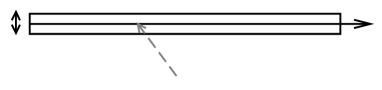
Figure 1. $\gamma_{j}$ as the center of tube $T^{\delta}_{j}$.

We consider the following two scenarios.

• I.(Low multiplicity scenario) Let $N_{1}$ be a nonnegative integer such that there are at least $\frac{M}{2}$ many $j$’s satisfying

  $$\Big{|}T^{\delta}_{j}\cap E\cap\Big{\{}x\in\mathbb{R}^{d}:\sum^{M}_{l=1,l\neq j}\chi_{T^{\delta}_{l}}(x)\leq N_{1}\Big{\}}\Big{|}\geq\frac{\lambda}{4}|T^{\delta}_{j}|;$$

• II_θσ.(High multiplicity at angle $\theta$ and distance $\sigma$). Let $N_{2}$ be a nonnegative integer such that for $\theta,\sigma\in[\delta,1]$ and $\mathcal{I}_{\theta,\sigma}(x,j)$ defined as in (2.5)

  $$\text{Card}\Big{\{}j:\Bigl{|}T^{\delta}_{j}\cap E\cap\Big{\{}x:\text{Card}\,\mathcal{I}_{\theta,\sigma}(x,j)\geq 2^{-3}\Big{(}\log_{2}\frac{1}{\delta}\Big{)}^{-2}N_{2}\Big{\}}\Bigr{|}\geq 2^{-3}\Big{(}2\log_{2}\frac{1}{\delta} \Big{)}^{-2}\lambda|T^{\delta}_{j}|\Big{\}}$$

  $$\geq\frac{M}{2^{4}(\log_{2}\frac{1}{\delta})^{2}}.$$

It is easy to see that $N_{1}\geq M$ is sufficient for scenario I. If we denote by $N$ the smallest $N_{1}$ such that scenario I is valid, then there exist $\theta,\sigma\in[\delta,1]$ such that II_θσ also holds for $N_{2}=N$. Essentially, this is achieved by using a dyadic pigeonhole principle. To see this, by the minimality of $N$ and triangle inequality, we have at least $\frac{M}{2}+1$ many $j$’s such that

$$\Big{|}\mathcal{Q}^{\delta}_{j}:=T^{\delta}_{j}\cap E\cap\Bigl{\{}x:\sum^{M}_{l=1,l\neq j}\chi_{T^{\delta}_{l}}\geq N\Bigr{\}}\Big{|}\geq\frac{\lambda}{4}|T^{\delta}_{j}|.$$ (2.6)

For any $x\in\mathcal{Q}^{\delta}_{j}$, we have

$$\sum^{M}_{l=1,l\neq j}\chi_{T^{\delta}_{l}}(x)\geq N,$$ (2.7)

and

$$\Bigl{\{}k:k\neq j,\,x\in T^{\delta}_{k}\Bigr{\}}\subset\bigcup^{[\log_{2}\frac{1}{\delta}]+1}_{\nu=1}\Bigl{\{}i:x\in T^{\delta}_{i},\angle(T^{\delta}_{j},T^{\delta}_{i})\in[2^{\nu-1}\delta,2^{\nu}\delta)\Bigr{\}}.$$ (2.8)

On the other hand, we claim that

$$\{k:k\neq j,\,x\in T^{\delta}_{k}\}$$ (2.9)

$$\subset\bigcup^{[\log_{2}\frac{2}{\delta}]}_{\nu^{\prime}=1}\Big{\{}i:x\in T^{\delta}_{i},\Big{|}T^{\delta}_{i}\cap\{y\in E:\text{dist}(y,\gamma_{j})\in[2^{\nu^{\prime}-1}\delta,2^{\nu^{\prime}}\delta)\}\Big{|}\geq\bigl{(}2^{4}\log_{2}\frac{1}{\delta}\bigr{)}^{-1}\lambda|T^{\delta}_{i}|\Big{\}}.$$

On account of (2.8) and (2.9), we may write

$$\{k:k\neq j,\,x\in T^{\delta}_{k}\}$$

$$\subset\bigcup^{[\log_{2}\frac{1}{\delta}]+1}_{\nu=1}\bigcup^{[\log_{2}\frac{2}{\delta}]}_{\nu^{\prime}=1}\Big{(}\{i:x\in T^{\delta}_{i},\angle(T^{\delta}_{j},T^{\delta}_{i})\in[2^{\nu-1}\delta,2^{\nu}\delta)\}$$

$$\quad\quad\quad\quad\quad\quad\quad\cap\Big{\{}i:x\in T^{\delta}_{i},\Big{|}T^{\delta}_{i}\cap\{y\in E:\text{dist}(y,\gamma_{j})\in[2^{\nu^{\prime}-1}\delta,2^{\nu^{\prime}}\delta)\}\Big{|}\geq\bigl{(}2^{4}\log_{2}\frac{1}{\delta}\bigr{)}^{-1}\lambda|T^{\delta}_{i}|\Big{\}}\Big{)}$$

$$\subset\bigcup^{[\log_{2}\frac{1}{\delta}]+1}_{\nu=1}\bigcup^{[\log_{2}\frac{2}{\delta}]}_{\nu^{\prime}=1}\mathcal{I}_{2^{\nu}\delta,2^{\nu^{\prime}}\delta}(x,j).$$

In view of (2.7), we have at least $N$ many tubes $T^{\delta}_{k}$ containing $x$ such that $k\neq j$. By choosing $\delta\ll 0.01$, we have

$$N\leq 2^{3}\Big{(}\log_{2}\frac{1}{\delta}\Big{)}^{2}\sup_{\begin{subarray}{c}1\leq\nu\leq[\log_{2}\frac{1}{\delta}]+1\\ 1\leq\nu^{\prime}\leq[\log_{2}{\frac{2}{\delta}}]\end{subarray}}\text{Card}\;\mathcal{I}_{2^{\nu}\delta,2^{\nu^{\prime}}\delta}(x,j).$$

Therefore, there are $\nu$ and $\nu^{\prime}$, which may depend on $x$ and $j$, such that

$$\text{Card}\;\mathcal{I}_{2^{\nu}\delta,2^{\nu^{\prime}}\delta}(x,j)\geq 2^{-3}\Big{(}\log_{2}\frac{1}{\delta}\Big{)}^{-2}N.$$

From the above discussions, we have

$$\mathcal{Q}^{\delta}_{j}\subset\bigcup^{[\log_{2}\frac{1}{\delta}]+1}_{\nu=1}\bigcup^{[\log_{2}\frac{2}{\delta}]}_{\nu^{\prime}=1}\Big{(}T^{\delta}_{j}\cap E\cap\Bigl{\{}x:\text{Card}\;\mathcal{I}_{2^{\nu}\delta,2^{\nu^{\prime}}\delta}(x,j)\geq 2^{-3}\Big{(}\log_{2}\frac{1}{\delta}\Big{)}^{-2}N\Bigr{\}}\Big{)},$$

which, by (2.6), yields

$$\frac{\lambda}{4}|T^{\delta}_{j}|\leq 2^{3}\Big{(}\log_{2}\frac{1}{\delta}\Big{)}^{2}\sup_{\nu,\nu^{\prime}}\Big{|}T^{\delta}_{j}\cap E\cap\Bigl{\{}x:\text{Card}\;\mathcal{I}_{2^{\nu}\delta,2^{\nu^{\prime}}\delta}(x,j)\geq 2^{-3}\Big{(}\log_{2}\frac{1}{\delta}\Big{)}^{-2}N\Bigr{\}}\Big{|}.$$

Consequently, we have found $\nu=\nu(j)$ and $\nu^{\prime}=\nu^{\prime}(j)$ such that

$$\Big{|}T^{\delta}_{j}\cap E\cap\Big{\{}x:\text{Card}\;\mathcal{I}_{2^{\nu}\delta,2^{\nu^{\prime}}\delta}(x,j)\geq 2^{-3}\Big{(}\log_{2}\frac{1}{\delta}\Big{)}^{-2}N\Big{\}}\Big{|}\geq 2^{-3}\lambda\Bigl{(}2\log_{2}\frac{1}{\delta}\Bigr{)}^{-2}|T^{\delta}_{j}|$$ (2.10)

Since there are at most $2^{4}\Big{(}\log_{2}\frac{1}{\delta}\Big{)}^{2}$ many pairs of $(\nu,\nu^{\prime})$’s and at least $\frac{M}{2}+1$ many $j$’s as in (2.10), by pigeonhole’s principle there is a pair $(\nu_{0},\nu^{\prime}_{0})$ such that II_θσ holds for $\theta=2^{\nu_{0}}\delta$ and $\sigma=2^{\nu^{\prime}_{0}}\delta$.

It remains to prove (2.9). For $k\neq j$, we have

$$\frac{\lambda}{2}|T^{\delta}_{k}|\leq|T^{\delta}_{k}\cap E|\leq 2 \sum^{[\log_{2}\frac{2}{\delta}]}_{\nu^{\prime}=1}\Bigl{|}T^{\delta}_{k}\cap E\cap\Bigl{\{}y:\text{dist}(y,\gamma_{j})\in[2^{\nu^{\prime}-1}\delta,2^{\nu^{\prime}}\delta)\Bigr{\}}\Bigr{|}$$

$$\leq 8 \log_{2}{\frac{1}{\delta}}\quad\sup_{\nu^{\prime}}\Big{|}T^{\delta}_{k}\cap E\cap\Bigl{\{}y:\text{dist}(y,\gamma_{j})\in[2^{\nu^{\prime}-1}\delta,2^{\nu^{\prime}}\delta)\Bigr{\}}\Big{|}$$

where we have used the fact that $k\neq j$ implies $\angle(T^{\delta}_{k},T^{\delta}_{j})\geq c\delta$ for some $c>0$ suitably large. Thus (2.9) follows.

Remark 2.1.

The high and low multiplicity scenarios for tubes was first exploited by Wolff [16]. This along with the the argument of induction on scales improves significantly the bound on Kakeya type maximal functions. The modified version in the above form was in spirit of Sogge [11]. Combining this with an $L^{2}-$estimate for an auxiliary maximal function, one may establish the Nikodym type maximal inequality in curved background with constant curvatures.

3. An auxiliary maximal function inequality

Let $\gamma_{j}$ be the central axis of $T^{\delta}_{j}$ as shown in Figure 1. We may assume without loss of generality that $\gamma_{j}$ is parallel to $e_{1}$, where $\{e_{1},e_{2},\ldots,e_{d}\}$ is the orthogonal normal basis of $\mathbb{R}^{d}$. For $y\in\mathbb{R}^{d}$, denote by $y=(y_{1},y^{\prime})$ with $y^{\prime}=(y_{2},\ldots,y_{d})$. In this section, we always assume that $f$ is an integrable function $\mathbb{R}^{d}$ supported in the hollow cylinder $\{y\in\mathbb{R}^{d}:|y_{1}|\leq 1,\,\frac{\sigma}{2}\leq|y^{\prime}|\leq\sigma\}$.

For any $\xi\in A_{\lambda}$ and a tube $T_{\xi}^{\delta}$ in the direction of $\xi$ such that $\angle(\xi,\xi^{j})>0$ and $T^{\delta}_{j}\cap T^{\delta}_{\xi}\neq\emptyset$, there is a unique point $q=q(j,\,\xi)$ such that

$$\text{dist}(q,\gamma_{j})+\text{dist}(q,\gamma_{\xi})=\min_{x\in\mathbb{R}^{d}}\Bigl{[}\text{dist}(x,\gamma_{j})+\text{dist}(x,\gamma_{\xi})\Bigr{]},$$ (3.1)

where $\gamma_{\xi}$ is the central axis of the tube $T^{\delta}_{\xi}$ in the direction $\xi$. We denote by $\gamma_{j}\wedge\gamma_{\xi}$ the point $q$ such that (3.1) holds. Let $\omega^{j}_{\xi}(y)=\big{[}\text{dist}(y,\gamma_{j}\wedge\gamma_{\xi})\big{]}^{\frac{1}{2}}$. For brevity, we write $\omega^{j}_{\xi^{\nu}}$ and $\gamma_{\xi^{\nu}}$ respectively as $\omega^{j}_{\nu}$ and $\gamma_{\nu}$.

Define the auxiliary maximal function as

$$A^{\theta}_{\delta,j}(f)(\xi)=\sup_{\begin{subarray}{c}T^{\delta}_{j}\cap T^{\delta}_{\xi}\neq\emptyset\\ \angle(T^{\delta}_{j},T^{\delta}_{\xi})\in[\frac{\theta}{2},\theta]\end{subarray}}\frac{1}{|T^{\delta}_{\xi}|}\int_{T^{\delta}_{\xi}}|f(y)|\omega^{j}_{\xi}(y)dy,$$

We define $A^{\theta}_{\delta,j}(f)(\xi)$ to be zero if $\angle(T^{\delta}_{j},T^{\delta}_{\xi})$ is outside the interval $[\frac{\theta}{2},\theta]$.

The difference between this auxiliary maximal function and $f^{*}_{\delta}$ is that the supremum is taken under more constraints for the tubes in direction of $\xi$. Besides, we put a weight function for technical reasons. On one hand, it is clear that $A^{\theta}_{\delta,j}(f)(\xi)\lesssim f^{*}_{\delta}(\xi)$ when $f$ is supported in a unit ball. On the other hand, a more interesting fact is that we can estimate the $L^{2}$ norm of $A^{\theta}_{\delta,j}(f)$ by means of $(d-1)-$dimensional Kakeya maximal functions. Thus, we reduce the problem of dimension $d$ to the problem of dimension $(d-1)$. In this sense, our argument is very similar to Bourgain’s induction on dimension argument in [1]. To be more specific, we prove in this section

Proposition 3.1.

Let $A^{\theta}_{\delta,j}(f)(\xi)$ be as above, we have for all $j$

$$\|A^{\theta}_{\delta,j}(f)\|_{L^{2}(S^{d-1})}\leq 2^{10}C_{\delta,d-1}\delta^{-\frac{d-3}{2}}\|f\|_{L^{2}(\mathbb{R}^{d})},$$ (3.2)

where $C_{\delta,d-1}$ is as in (1.5).

Proof.

Without loss of generality, we let $j=0,\xi^{0}=e_{1}$ and suppress the subscript $j$ and superscript $\theta$ in $A^{\theta}_{\delta,j}$. By symmetry, we only consider the following integral

$$\int_{S^{d-1}_{+}}|A_{\delta}(f)|^{2}(\xi)d\Sigma(\xi),$$ (3.3)

where $d\Sigma$ represents the standard surface measure on the unit sphere and

$$S^{d-1}_{+}=\{\xi\in S^{d-1}\mid\xi_{1}\geq 0\}.$$

    $$5\delta v_{k} O \mathcal{C}_{\theta} H_{k}$$

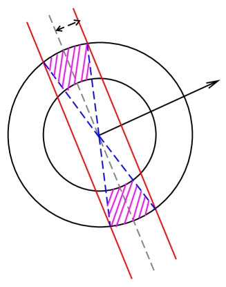
Figure 2. The angular decomposition for $\mathcal{C}_{\theta}$.

Since $\angle(\xi,e_{1})\in[\frac{\theta}{2},\theta]$, we may restrict $\sin\frac{\theta}{2}\leq|\xi^{\prime}|\leq\sin\theta$ in the integration of (3.3) with respect to $\xi=(\xi_{1},\xi^{\prime})$. Let

$$\mathcal{C}_{\theta}=\Bigl{\{}\xi^{\prime}=(\xi_{2},\ldots,\xi_{d})\in\mathbb{R}^{d-1}:\sin\frac{\theta}{2}\leq|\xi^{\prime}|\leq\sin\theta\Bigr{\}},$$

and take a maximal $\frac{\delta}{\theta}-$separated subset $\{v_{k}\}^{\sim(\theta/\delta)^{d-2}}_{k=1}$ of $S^{d-2}$, which is the unit sphere in $\mathbb{R}^{d-1}_{\xi^{\prime}}$. Define

$$\Pi^{\delta,\theta}_{k}=\Big{\{}\xi^{\prime}\in\mathcal{C}_{\theta}:\Bigl{|}\Bigl{\langle}\frac{\xi^{\prime}}{|\xi^{\prime}|},v_{k}\Bigr{\rangle}\Bigr{|}\leq\frac{\delta}{2}\Big{\}},$$

which is contained in a $5\delta-$neighborhood of the $(d-2)-$dimensional hyperplane $H_{k}$ perpendicular to $v_{k}$. Next, we define $\Gamma^{\delta,\theta}_{1}=\Pi^{\delta,\theta}_{1},$ and $\Gamma^{\delta,\theta}_{k}=\Pi^{\delta,\theta}_{k}\setminus\Big{(}\bigcup^{k-1}_{j=1}\Pi^{\delta,\theta}_{j}\big{)}$ for $k\geq 2$. Then we have $\mathcal{C}_{\theta}\subset\bigcup_{k}\Gamma^{\delta,\theta}_{k}$ and $\Gamma^{\delta,\theta}_{k}\cap\Gamma^{\delta,\theta}_{k^{\prime}}=\emptyset$ for $k\neq k^{\prime}$.

If $\xi^{\prime}\in\Gamma^{\delta,\theta}_{k}$ for some $k\in\Bigl{\{}1,\ldots,\sim\Big{(}\frac{\theta}{\delta}\Big{)}^{d-2}\Bigr{\}}$, then the tube $T^{\delta}_{\xi}$, in direction of $\xi=(\sqrt{1-|\xi^{\prime}|^{2}},\xi^{\prime})\in S^{d-1}$ must lie in a $50\delta-$neighborhood $\tilde{H}^{50\delta}_{k}$ of the hyperplane $\tilde{H}_{k}:=\text{span}\{e_{1},H_{k}\}$, since $T^{\delta}_{\xi^{0}}\cap T^{\delta}_{\xi}\neq\emptyset$.

    $$e_{1} T^{\delta}_{\xi} \xi \Gamma^{\delta,\theta}_{k} O v_{k} H_{k}$$

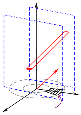
Figure 3. $T^{\delta}_{\xi}$ is contained in $\tilde{H}^{50\delta}_{k}$.

From this observation, we introduce the following cylindrical sets

$$\mathcal{V}_{k}=\{y\in\mathbb{R}^{d}:|y_{1}|\leq 1,\,|\langle y^{\prime},v_{k}\rangle|<50\delta\}.$$

Then we have the following almost orthogonality estimate

$$\sum_{k}\chi_{\mathcal{V}_{k}\cap\text{supp}f}(y)\leq C\frac{\theta^{d-2}}{\delta^{d-3}\sigma}.$$ (3.4)

To see this, for any $y^{\prime}$ such that $\frac{\sigma}{2}\leq|y^{\prime}|\leq\sigma$ and denote by $H^{50\delta}_{k}$ the $50\delta-$neighborhood of $H_{k}$. Let $\Pi_{y^{\prime}}$ be the hyperplane in $\mathbb{R}^{d-1}$ perpendicular to $y^{\prime}$. One easily verifies that $H^{50\delta}_{k}$ contains $y^{\prime}$ only when $v_{k}\in S^{d-2}$ lives in a $\frac{100\delta}{\sigma}-$neighborhood of $\Pi_{y^{\prime}}$. Thus there are at most $O\bigl{(}\frac{\theta^{d-2}}{\sigma\delta^{d-3}}\bigr{)}$ many $H^{50\delta}_{k}$’s containing $y^{\prime}$ simultaneously.

Now we turn to estimate (3.3). This will be reduced to the following maximal function $\mathcal{A}_{\delta}$ defined similar to $A_{\delta}$,

$$\mathcal{A}_{\delta}(f)(\xi)\mathrel{\mathop{=}^{\rm def}}\sup_{\begin{subarray}{c}T^{\delta}_{0}\cap T^{\delta}_{\xi}\neq\emptyset\\ \angle(T^{\delta}_{0},T^{\delta}_{\xi})\in[\frac{\theta}{2},\theta]\end{subarray}}\frac{1}{|T^{\delta}_{\xi}|}\int_{T^{\delta}_{\xi}}|f(y)|dy.$$

For the moment, we assume that for each $k\in\Big{\{}1,\ldots,\sim\Big{(}\frac{\theta}{\delta}\Big{)}^{d-2}\Big{\}}$

$$\|\mathcal{A}_{\delta}(f\chi_{\mathcal{V}_{k}})\|_{L^{2}(\{\xi\in S^{d-1}_{+}\mid\,\xi^{\prime}\in\Gamma^{\delta,\theta}_{k}\})}\leq C_{\delta,d-1}\|f\chi_{\mathcal{V}_{k}}\|_{L^{2}}.$$ (3.5)

We next deduce (3.2) under the assumption (3.5). Noting that for $\theta\leq 1$,

$$\frac{1}{\sqrt{1-\sin^{2}\theta}}\leq 2,$$

and

$$\omega_{\xi}(y)\sim\Big{(}\frac{\sigma}{\theta}\Big{)}^{\frac{1}{2}},\quad\forall y\in\mathcal{V}_{k}\cap T^{\delta}_{\xi}\cap\text{supp}f,\;\forall\xi^{\prime}\in\Gamma^{\delta,\theta}_{k},$$

we estimate (3.3) in the following manner

$$\eqref{3.1} \leq 4\int_{\mathcal{C}_{\theta}}|A_{\delta}(f)|^{2}(\sqrt{1-|\xi^{\prime}|^{2}},\xi^{\prime})d\xi^{\prime}\leq 4\sum_{k}\int_{\Gamma^{\delta,\theta}_{k}}|A_{\delta}(f\chi_{\mathcal{V}_{k}})|^{2}(\xi^{\prime})d\xi^{\prime}$$

$$\lesssim\frac{\sigma}{\theta}\sum_{k}\int_{\Gamma^{\delta,\theta}_{k}}|\mathcal{A}_{\delta}(f\chi_{\mathcal{V}_{k}})|^{2}(\xi^{\prime})d\xi^{\prime}\lesssim\frac{\sigma}{\theta}C^{2}_{\delta,d-1}\sum_{k}\int_{\mathbb{R}^{d}}|f|^{2}\chi_{\mathcal{V}_{k}}(y)dy\lesssim C^{2}_{\delta,d-1}\Big{(}\frac{\theta}{\delta}\Big{)}^{d-3}\|f\|^{2}_{2},$$

where the last inequality is due to (3.4).

    $$T^{\delta}_{\xi} \mathcal{T}^{\delta}_{\xi}$$

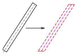
Figure 4. $T^{\delta}_{\xi}$;  and  $\mathcal{T}^{\delta}_{\xi}$.

Therefore, we are reduced to proving (3.5). By rotation invariance, we may assume $k=1$ and $v_{1}$ is identical to $e_{d}$. We may assume further that $f$ is supported in $\mathcal{V}_{1}$. Clearly, $\Gamma^{\theta,\delta}_{1}$ is contained in the region

$$\Theta^{\theta,\delta}_{1}:=\Big{\{}\xi^{\prime}\in\mathbb{R}^{d-1}:|(\xi_{2},\ldots,\xi_{d-1})|\leq\sin\theta,\,|\xi_{d}|\leq 10\delta\Big{\}}.$$

Fix $\xi^{\prime}\in\Theta^{\theta,\delta}_{1}$ and denote by $p\in\gamma_{\xi}$ such that $p$ is closest to $\gamma_{\xi}\wedge\gamma_{0}$ with $p=(p_{1},p^{\prime})$. We slightly modify $T^{\delta}_{\xi}(a)$ to be $\mathcal{T}^{\delta}_{\xi}(a)$ as follows, singling out $y_{1}$ as the parameter of the central axis (see Figure 4)

$$\mathcal{T}^{\delta}_{\xi}=\Big{\{}(y_{1},y^{\prime})\in\mathbb{R}\times\mathbb{R}^{d-1}: \,\Big{|}y^{\prime}-p^{\prime}-\frac{y_{1}-p_{1}}{\sqrt{1-|\xi^{\prime}|^{2}}}\xi^{\prime}\Big{|}\leq\frac{\delta}{2\sqrt{1-|\xi^{\prime}|^{2}}},$$

$$p_{1}-(\frac{1}{2}-\text{dist}(a,p))\cos\alpha\leq y_{1}\leq p_{1}+(\frac{1}{2}+\text{dist}(a,p))\cos\alpha\Big{\}}.$$

where $a=(a_{1},a^{\prime})$ is the middle of $\gamma_{\xi}$ and $\alpha:=\angle(\gamma_{0},\gamma_{\xi})$.

Let $\mathcal{P}(y_{d})$ be the hyperplane perpendicular to $v_{1}$ and parameterized by $y_{d}$. Fix $y_{d}\in[-50\delta,50\delta]$ and consider $\mathcal{P}(y_{d})\bigcap\mathcal{T}^{\delta}_{\xi}:=\mathcal{E}_{\delta}(y_{d})$. One can verify that $\mathcal{E}_{\delta}$ is an ellipse with major axis at least $1/10$. In fact, let $\beta$ be the angle between $\mathcal{T}^{\delta}_{\xi}$ and $v_{1}$.

    $$\beta \frac{\pi}{2}-\beta \mathcal{E}_{\delta}(y_{d}) \xi$$

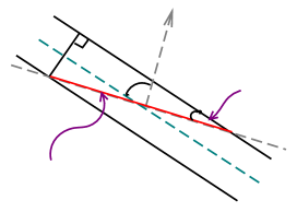
Figure 5. The ellipsoid $\mathcal{E}_{\delta}(y_{d})$.

We have $\cos\beta=\xi_{d}$, which implies the major axis is at least $\frac{\delta}{\sin(\frac{\pi}{2}-\beta)}\geq\frac{\delta}{|\xi_{d}|}\geq\frac{1}{10}$. Thus $\mathcal{E}_{\delta}(y_{d})$ can be regarded as a $(d-1)-$dimensional Kakeya tube with dimensions $1\times\underbrace{\delta\times\ldots\times\delta}_{d-2}$.

Let $r=(1-\xi^{2}_{d})^{\frac{1}{2}}$ and $\xi^{{}^{\prime\prime}}=(\xi_{2},\ldots,\xi_{d-1})$. Since $|\xi^{{}^{\prime\prime}}|\leq\sin\theta\leq\frac{\sqrt{3}}{2}$ and $|r-1|\ll 1$ by taking $\delta$ sufficiently small, we see that $(\sqrt{r^{2}-|\xi^{{}^{\prime\prime}}|^{2}},\xi^{{}^{\prime\prime}})$ represents a vector on $rS^{d-2}$. By Fubini’s theorem, the integral average of $f$ over $\mathcal{T}^{\delta}_{\xi}$ is controlled by

$$\delta^{-(d-1)}\int_{|y_{d}|\leq 50\delta}dy_{d}\int_{\mathcal{E}_{\delta}(y_{d})}|f(y_{1},\ldots,y_{d-1},y_{d})|dy_{1}\ldots dy_{d-1}.$$

Next, we use the $(d-1)-$dimensional Kakeya maximal functions to bound the above formula. In particular, this implies

$$\mathcal{A}_{\delta}(f)(\xi^{\prime})\lesssim\delta^{-1}\int_{|y_{d}|\leq 50\delta}M_{\delta}(f(\ldots,y_{d}))(\sqrt{r^{2}-|\xi^{{}^{\prime\prime}}|^{2}},\xi^{{}^{\prime\prime}})dy_{d},$$

where $M_{\delta}(f(\ldots,y_{d}))$ denotes the $(d-1)-$dimensional Kakeya maximal operator acting on $f$, and $f$ is regarded as a function of the $d-1$ variables $(y_{1},\ldots,y_{d-1})$ with $y_{d}$ frozen as a parameter.

Using Minkowski’s inequality and Hölder’s inequalities, we obtain by $r<1$

$$\left(\int_{|(\xi_{2},\ldots,\xi_{d-1})|\leq\sin\theta}|\mathcal{A}_{\delta}(f)(\xi^{\prime})|^{2}d\xi_{2}\ldots d\xi_{d-1}\right)^{\frac{1}{2}}$$

$$\leq\delta^{-1}\int_{|y_{d}|\leq 50\delta}\left(\int|M_{\delta}(f(\ldots,y_{d}))|^{2}(\sqrt{r^{2}-|\xi^{{}^{\prime\prime}}|^{2}},\xi^{{}^{\prime\prime}})d\xi_{2}\ldots d\xi_{d-1}\right)^{\frac{1}{2}}dy_{d}$$

$$\leq 2\delta^{-1}\int_{|y_{d}|\leq 50\delta}\left(\|M_{\delta}(f(\ldots,y_{d}))\|^{2}_{L^{2}(S^{d-2})}\right)^{\frac{1}{2}}dy_{d}$$

$$\leq 2\delta^{-1}C_{\delta,d-1}\int_{|y_{d}|\leq 50\delta}\|f(\ldots,y_{d})\|_{L^{2}_{y_{1},\ldots,y_{d-1}}}dy_{d}$$

$$\leq 2^{6}\delta^{-1/2}C_{\delta,d-1}\|f\|_{2}.$$

Squaring both sides and integrating with respect to $\xi_{d}\in[-10\delta,10\delta]$, we get (3.5) and hence (3.2). ∎

It is well-knownthat $C_{\delta,2}=\log\frac{1}{\delta}$ , and consequently we conclude

Corollary 3.2.

If $d=3$, we have for some $c>0$

$$\|A^{\theta}_{\delta,j}(f)\|_{L^{2}(S^{2})}\leq c\Big{(}\log\frac{1}{\delta}\Big{)}\|f\|_{L^{2}(\mathbb{R}^{3})}.$$ (3.6)

This corollary is crucial in the proof of Theorem 1.

Remark 3.3.

We observe some essential distinctions between the 3D and higher dimensional problems. Indeed, we find in Proposition 3.1 that the loss of the factor $\delta^{-\frac{d-3}{2}}$ vanishes in the three dimensional case. This allows us to use the optimal estimates on 2D Kakeya maximal function to deduce Wolff’s $L^{\frac{5}{2}}-$bound on the 3D case. On the other hand, we do not know whether the $\delta^{-\frac{d-3}{2}}$ loss is necessary in (3.2). Since our method of reducing the estimate on $d$-dimensional auxiliary maximal function to the estimates of $(d-1)-$dimensional Kakeya maximal function is rather crude, it seems possible by strengthening the argument to reduce the $\frac{d-3}{2}-$exponent of the loss. This might be easier when $d$ is large, while for lower dimensions, it seems rather difficult.

4. The key Lemmas

Lemma 4.1.

Let $N$ satisfy scenario I, then $|E|\geq\lambda M\delta^{d-1}(16N)^{-1}$.

Proof.

Relabeling the subscripts, we may write the tubes involved in case I as $\{T^{\delta}_{j}\}^{K}_{j=1}$ with $M\geq K\geq M/2$. Then, we have

$$\frac{\lambda M\delta^{d-1}}{8N} \leq\frac{\lambda}{4N}\sum^{K}_{j=1}|T^{\delta}_{j}|\leq\frac{1}{N}\sum^{K}_{j=1}\Bigl{|}T^{\delta}_{j}\cap E\cap\Bigl{\{}x\in\mathbb{R}^{d}\mid\sum^{M}_{\ell=1,\ell\neq j}\chi_{T^{\delta}_{\ell}}(x)\leq N\Bigr{\}}\Bigr{|}$$

$$\leq\int_{E\cap\bigl{\{}x\in\mathbb{R}^{d}:\,\sum\limits_{\ell=1,\ldots,M}\chi_{T^{\delta}_{\ell}}(x)\leq N+1\bigr{\}}}\frac{1}{N}\sum^{K}_{j=1}\chi_{T^{\delta}_{j}}(x)dx\leq 2|E|.$$

∎

Lemma 4.2.

Suppose there are $M$ many tubes $\{T^{\sigma}_{j}\}^{M}_{j=1}$ such that $j\neq j^{\prime}$ and $T^{\sigma}_{j}\cap T^{\sigma}_{j^{\prime}}\neq\emptyset$ implies $\angle(T^{\sigma}_{j},T^{\sigma}_{j^{\prime}})\geq\gamma$ for some $0<\gamma<\frac{\pi}{2}$. Assume also that for some $\rho>0$ and any $a\in\mathbb{R}^{d}$, there are $M_{0}$ many of such tubes satisfying

$$\rho|T^{\sigma}_{j}|\leq\Big{|}T^{\sigma}_{j}\cap E\cap B(a,\sigma/\gamma)^{c}\Big{|}.$$ (4.1)

Then we have

$$|E|\geq\rho\sigma^{d-1}M^{1/2}_{0}/2.$$ (4.2)

Proof.

By relabeling the indices, we have, under these assumptions, a sequence $\{T^{\sigma}_{j}\}^{M_{0}}_{j=1}$ satisfying

$$\rho\sigma^{d-1}M_{0}\leq\int_{E}\sum^{M_{0}}_{j=1}\chi_{T^{\sigma}_{j}}(x)dx.$$

Thus, there exists an $x_{0}\in E$ such that

$$\sum^{M_{0}}_{j=1}\chi_{T^{\sigma}_{j}}(x_{0})\geq\frac{\rho\sigma^{d-1}M_{0}}{2|E|}.$$

We relabel the subcollection of the tubes $\{T^{\sigma}_{j}\}_{j\in\{1,\ldots,C_{*}\}}$ containing $x_{0}$, where

$$C_{*}=C_{\rho,\sigma,M_{0},E}=\Big{[}\frac{\rho\sigma^{d-1}M_{0}}{2|E|}\Big{]}.$$

We notice the orthogonality outside the ball $B(x_{0},\sigma/\gamma)$ by the following observation. It follows from the angle condition in the assumptions that the component of $T^{\sigma}_{j}\cap T^{\sigma}_{j^{\prime}}$ must be contained in the ball $B(x_{0},L)$ with $L$ at most $\frac{\sigma}{2}/\sin{\frac{\gamma}{2}}$, which is less than $\sigma/\gamma$ for $\gamma<\frac{\pi}{2}$. With the help of this orthogonality, the choice of $C_{*}$ and (4.1), we have

$$|E| \geq\Bigl{|}E\cap B(x_{0},\sigma/\gamma)^{c}\cap\bigcup^{C_{*}}_{j=1}T^{\sigma}_{j}\Bigr{|}\geq\sum^{C_{*}}_{j=1}|E\cap B(x_{0},\sigma/\gamma)^{c}\cap T^{\sigma}_{j}|$$

$$\geq C_{*}\rho\sigma^{d-1}\geq\frac{\rho^{2}\sigma^{2(d-1)}M_{0}}{4|E|},$$

where we use Lemma 4.1 in the last inequality.

∎

    $$T^{\sigma}_{j} x_{0} B(x_{0},\sigma/\gamma) T^{\sigma}_{j^{\prime}}$$

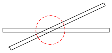
Figure 6. The orthogonality of tubes outside a ball $B(x_{0},\sigma/\gamma)$.

Lemma 4.3.

Let $N$ satisfy both case I and case II_θσ. Then, there are $M2^{-4}\Big{(}\log_{2}\frac{1}{\delta}\Big{)}^{-2}$ many tubes $T^{\delta}_{j}$ in II_θσ. Suppose for any $\varepsilon>0$, there exists $C_{\varepsilon}>0$ such that for small $\delta>0$ and any point $a\in\mathbb{R}^{d}$,

$$|E\cap B(a,\delta^{\varepsilon}\lambda^{d-2})^{c}\cap T^{\sigma}_{j}|\geq C_{\varepsilon}\lambda^{3}\sigma\delta^{d-2+\varepsilon}N,$$ (4.3)

then we have (2.4).

Proof.

We rewrite (2.4) as $|E|^{2}\geq C_{\varepsilon}\lambda^{d+2}\Big{(}\delta^{d-1}M\Big{)}^{\frac{d}{d-1}}\delta^{d-2+\varepsilon}$. Then it suffices to prove

$$|E|\geq\lambda M\delta^{d-1}(16N)^{-1},$$ (4.4)

and

$$|E|\geq C_{\varepsilon}\lambda^{d+1}N(\delta^{d-1}M)^{\frac{1}{d-1}}\delta^{d-2+\varepsilon},$$ (4.5)

where (4.4) is proved in Lemma 4.1 and it remains to prove (4.5). Let $\{\xi_{j}\}_{j\in\{1,\ldots,[M2^{-4}(\log_{2}\frac{1}{\delta})^{-2}]\}}$ be the directions of $T^{\delta}_{j}$. Noting that $\sigma\geq\delta$, we have $\gamma:=\frac{100\sigma}{\delta^{\varepsilon}\lambda^{d-2}}\geq\delta^{1-\varepsilon}$ since $\lambda\leq 1$ and $d\geq 3$. If $\gamma\geq\frac{\pi}{2}$, then (4.5) follows immediately from (4.3).

Otherwise, we can take a maximal $\gamma-$separated subsequence of $\{\xi_{j}\}$ and denote them by $\{\xi_{j_{k}}\}^{M_{0}}_{k=1}$. By maximality, we obtain for some $C_{2}>0$

$$M_{0}\geq C_{2}\frac{M}{2^{4}\Big{(}\log_{2}\frac{1}{\delta}\Big{)}^{2}}\delta^{d-1}\Big{(}\frac{\delta^{\varepsilon}\lambda^{d-2}}{\sigma 100}\Big{)}^{d-1}\geq C_{2}\frac{M\delta^{d-1}}{2^{4}\Big{(}\log_{2}\frac{1}{\delta}\Big{)}^{2}}\Big{(}\frac{\delta^{\varepsilon}\lambda^{d-2}}{\sigma 100}\Big{)}^{d-1}.$$

and use Lemma 4.2 with $\rho=C_{\varepsilon}\lambda^{3}\sigma^{2-d}\delta^{d-2+\varepsilon}N$ as well as (4.3) to get

$$|E| \geq C_{\varepsilon}\lambda^{3}\sigma^{2-d}\delta^{d-2+\varepsilon}N\times\sigma^{d-1}\times\frac{M^{\frac{1}{2}}_{0}}{2}$$

$$\geq\frac{C_{\varepsilon}}{2}\lambda^{3}\sigma\delta^{d-2+\varepsilon}N\times\Big{(}\frac{C_{2}}{4}M\delta^{d-1-\varepsilon c_{3}}\Big{)}^{\frac{1}{d-1}}\times\frac{\delta^{\varepsilon}\lambda^{d-2}}{\sigma 100}$$

$$\geq\tilde{C}_{\varepsilon}\lambda^{d+1}\delta^{d-2+(2+\frac{1}{d-1})\varepsilon}(M\delta^{d-1})^{\frac{1}{d-1}}N,$$

which implies (4.5), since $\varepsilon>0$ is arbitrarily small. ∎

Remark 4.4.

In the second step, we have used $M^{\frac{1}{2}}_{0}\geq M^{\frac{1}{d-1}}_{0}$ for $d\geq 3$. Since we can only verify (4.3) for $d=3$, this loss caused by cutting $\frac{1}{2}$ down to $\frac{1}{d-1}$ is dismissed. However, this loss appears to be significant when one deals with the higher dimensional cases with $d\geq 4$.

5. Completion of the proof to Theorem 1

In this section, we confine ourselves in the case when $d=3$ and prove (4.3) using Corollary 3.2. This will complete the proof of Wolff’s $L^{\frac{5}{2}}-$bound for Kakeya maximal functions. Before proving (4.3), we first prove a simplified version.

Lemma 5.1.

Let $d=3$ and $N$ satisfy both scenario I and II_θσ. Denote the $M2^{-4}\Big{(}\log_{2}\frac{1}{\delta}\Big{)}^{-2}$ many tubes by $\{T^{\delta}_{j}\}$ in II_θσ. For any $\varepsilon>0$, there exists a $C_{\varepsilon}>0$ such that for $\delta>0$ sufficiently small, we have

$$|E\cap T^{\sigma}_{j}|\geq C_{\varepsilon}\lambda^{3}\sigma\delta^{1+\varepsilon}N.$$ (5.1)

Proof.

For any $j\in\Big{\{}1,\ldots,\Big{[}M2^{-4}\Big{(}\log_{2}\frac{1}{\delta}\Big{)}^{-2}\Big{]}\Big{\}}$, we define

$$S^{\delta}_{j}\mathrel{\mathop{=}^{\rm def}}T^{\delta}_{j}\cap E\cap\left\{x:\text{Card}\;\mathcal{I}_{\theta,\sigma}(x,j)\geq 2^{-3}N\Big{(}\log_{2}\frac{1}{\delta}\Big{)}^{-2}\right\}.$$

By definition of $\mathcal{I}_{\theta,\sigma}(x,j)$, we see that there exists an $M_{0}\in(0,M]$ and a subcollection $\{T^{\delta}_{i_{k}}\}^{M_{0}}_{k=1}$ of $\{T^{\delta}_{i}\}^{M}_{i=1}$ such that

$$\angle(T^{\delta}_{i_{k}},T^{\delta}_{j})\in\Big{[}\frac{\theta}{2},\theta\Big{)},$$ (5.2)

$$\left|T^{\delta}_{i_{k}}\cap E\cap\left\{y:\text{dist}(y,\gamma_{j})\in\left[\frac{\sigma}{2},\sigma\right)\right\}\right|\geq\left(2^{4}\log_{2}\frac{1}{\delta}\right)^{-1}\lambda|T^{\delta}_{i_{k}}|,$$ (5.3)

and

$$\Big{(}\sum^{M_{0}}_{k=1}\chi_{T^{\delta}_{i_{k}}}\Big{)}\Big{|}_{S^{\delta}_{j}}\geq\frac{N}{2^{3}}\left(\log_{2}\frac{1}{\delta}\right)^{-2}.$$ (5.4)

Moreover, we have from the definition of II_θ,σ, (5.4) and $S^{\delta}_{j}\subset T^{\delta}_{j}$

$$2^{-3}\frac{\lambda}{(4\log_{2}\frac{1}{\delta})^{2}}|T^{\delta}_{j}| \leq|S^{\delta}_{j}|\leq 2^{3}\bigl{(}2\log_{2}\frac{1}{\delta}\bigr{)}^{2}N^{-1}\int_{T^{\delta}_{j}}\sum^{M_{0}}_{k=1}\chi_{T^{\delta}_{i_{k}}}(x)dx$$

$$\leq N^{-1}2^{3}\Big{(}2\log_{2}\frac{1}{\delta}\Big{)}^{2}\sum^{M_{0}}_{k=1}|T^{\delta}_{i_{k}}\cap T^{\delta}_{j}|\leq N^{-1}2^{3}\Big{(}\log_{2}\frac{1}{\delta}\Big{)}^{2}8\delta^{3}M_{0}/\theta,$$

where we have used $|T^{\delta}_{i_{k}}\cap T^{\delta}_{j}|\leq\frac{\delta^{3}}{\theta}$. Hnece we conclude

$$M_{0}\geq 2^{-10}\theta\delta^{-1}N\lambda\Big{(}\log_{2}\frac{1}{\delta}\Big{)}^{-4}.$$ (5.5)

    $$\sigma \frac{\sigma}{2} \theta \gamma_{j}\wedge\gamma_{i_{k}} \gamma_{j} \gamma_{i_{k}}$$

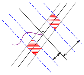
Figure 7. $T^{\delta}_{i_{k}}\cap\{y:\text{dist}(y,\gamma_{j})\in[\sigma/2,\sigma)\}$ is indicated by the shaded region.

Now, for any $T^{\delta}_{i_{k}}$, we have ( see Figure 7 )

$$|T^{\delta}_{i_{k}}|^{-1} \int_{T^{\delta}_{i_{k}}}\chi_{E\cap T^{\sigma}_{j}}(y)\omega^{j}_{i_{k}}(y)dy$$ (5.6)

$$\geq|T^{\delta}_{i_{k}}|^{-1}\int_{T^{\delta}_{i_{k}}\cap E\cap\{y:\text{dist}(y,\gamma_{j})\in[\sigma/2,\sigma)\}}[\text{dist}(y,\gamma_{i_{k}}\wedge\gamma_{j})]^{\frac{1}{2}}dy$$

$$\geq\left(\frac{\sigma}{\theta}\right)^{\frac{1}{2}}|T^{\delta}_{i_{k}}|^{-1}\cdot|T^{\delta}_{i_{k}}\cap E\cap\{y:\text{dist}(y,\gamma_{j})\in[\sigma/2,\sigma)\}|$$

$$\geq\Big{(}2^{4}\log_{2}\frac{1}{\delta}\Big{)}^{-1}\left(\frac{\sigma}{\theta}\right)^{\frac{1}{2}}\lambda.$$

On the other hand,

$$|T^{\delta}_{i_{k}}|^{-1}\int_{T^{\delta}_{i_{k}}}\chi_{E\cap T^{\sigma}_{j}}(y)\omega^{j}_{i_{k}}(y)dy\leq A^{\theta}_{\delta,j}(\chi_{E\cap T^{\sigma}_{j}})(\xi_{i_{k}}).$$

Squaring both sides, multiplying $\delta^{2}$ and summing up with respect to $k=1,\ldots,M_{0}$, we have

$$M_{0}\delta^{2}\Big{(}2\log_{2}\frac{1}{\delta}\Big{)}^{-2}\frac{\lambda^{2}\sigma}{\theta} \leq\sum^{M_{0}}_{k=1}\Big{|}A^{\theta}_{\delta,j}(\chi_{E\cap T^{\sigma}_{j}})(\xi_{i_{k}})\Big{|}^{2}\delta^{2}$$

$$\lesssim\int_{S^{2}}\Big{|}A^{\theta}_{\delta,j}(\chi_{E\cap T^{\sigma}_{j}})(\xi)\Big{|}^{2}d\Sigma(\xi)$$

$$\lesssim\bigl{(}\log\frac{1}{\delta}\bigr{)}|E\cap T^{\sigma}_{j}|,$$

where the last step involves the $L^{2}-$estimate (3.6).

Invoking the lower bound (5.5), we obtain (5.1). ∎

Proposition 5.2.

If $d=3$, then (4.3) holds.

Proof.

For $i\in\mathcal{I}_{\theta,\sigma}(x,j)$, we have by choosing $\delta$ small

$$\Big{|}T^{\delta}_{i}\cap\Big{\{}y\in E\cap B(a,\delta^{\varepsilon}\lambda)^{c} :\text{dist}(y,\gamma_{j})\in[\sigma/2,\sigma]\Big{\}}\Big{|}$$

$$\geq\Big{(}2^{4}\log_{2}\frac{1}{\delta}\Big{)}^{-1}\lambda|T^{\delta}_{i}|-\delta^{\varepsilon}\lambda|T^{\delta}_{i}|\geq\Big{(}2^{5}\log_{2}\frac{1}{\delta}\Big{)}^{-1}\lambda|T^{\delta}_{i}|.$$

If we define

$$\mathcal{\tilde{I}}_{\theta,\sigma}(x,j)\mathrel{\mathop{=}^{\rm def}} \Big{\{}i:\,\chi_{T^{\delta}_{i}}(x)=1,\,\angle(T^{\delta}_{i},T^{\delta}_{j})\in\Big{[}\frac{\theta}{2},\theta\Big{)},$$

$$\quad\quad\quad\quad\quad\quad\Big{|}T^{\delta}_{i}\cap\Big{\{}y\in E\cap B(a,\delta^{\varepsilon}\lambda)^{c}:\text{dist}(y,\gamma_{j})\in\Big{[}\frac{\sigma}{2},\sigma\Big{)}\Big{\}}\Big{|}\geq\Big{(}2^{5}\log_{2}\frac{1}{\delta}\Big{)}^{-1}\lambda|T^{\delta}_{i}|\Big{\}},$$

then, clearly $\mathcal{I}_{\theta,\sigma}(x,j)\subset\mathcal{\tilde{I}}_{\theta,\sigma}(x,j)$, which gives $\text{Card}\;\mathcal{I}_{\theta\sigma}(x,j)\leq\text{Card}\;\mathcal{\tilde{I}}_{\theta\sigma}(x,j)$. Since there are at least $M2^{-4}\Big{(}\log_{2}\frac{1}{\delta}\Big{)}^{-2}$ many $j$’s satisfying II_θσ, we have for each such $j$

$$2^{-3}\Big{(}4\log_{2}\frac{1}{\delta}\Big{)}^{-2}\lambda|T^{\delta}_{j}|\leq\left|\left\{x\in T^{\delta}_{j}\cap E\cap B(a,\delta^{\varepsilon}\lambda)^{c}:\text{Card}\,\mathcal{\tilde{I}}_{\theta,\sigma}(x,j)\geq 2^{-3}\Big{(}\log_{2}\frac{1}{\delta}\Big{)}^{-2}N\right\}\right|+\delta^{\varepsilon}\lambda|T^{\delta}_{j}|.$$

Taking $\delta$ small, we obtain for this $j$

$$2^{-3}\Big{(}4\log_{2}\frac{1}{\delta}\Big{)}^{-2}\frac{\lambda}{2}|T^{\delta}_{j}|\leq\left|\left\{x\in T^{\delta}_{j}\cap E\cap B(a,\delta^{\varepsilon}\lambda)^{c}:\text{Card}\,\mathcal{\tilde{I}}_{\theta,\sigma}(x,j)\geq\Big{(}2\log_{2}\frac{1}{\delta}\Big{)}^{-2}N\right\}\right|.$$

Replacing $E$ in lemma 5.1 with $E\cap B(a,\delta^{\varepsilon}\lambda)^{c}$ and using (5.1) with $\lambda/2$ instead of $\lambda$, we finally conclude (4.3) for $d=3$. Therefore, we complete the proof of of our main theorem. ∎

6. Appendix

6.1. The local property of Kakeya maximal function inequality

In this section, we shall see the problem on Kakeya maximal inequality is local. Namely, to derive (1.7), we can assume $f$ is supported in a ball of finite size. In particular, we may assume $f$ is supported in the unit ball centered at zero. To show that the general inequality (1.4) for $f$ defined on $\mathbb{R}^{d}$ follows from its localized version, we first choose a maximal $\delta-$separated subset $\{\xi^{k}\}_{k\in\mathfrak{K}}$ in $S^{d-1}$ with ${\rm Card}\mathfrak{K}\sim\delta^{-(d-1)}$, and write for a locally integrable function $f$

$$\int_{S^{d-1}}|f^{*}_{\delta}(\xi)|^{q}d\Sigma(\xi)\lesssim\sum_{k\in\mathfrak{K}}\int_{\angle(\xi,\xi^{k})\leq\delta}|f^{*}_{\delta}(\xi)|^{q}d\Sigma(\xi).$$ (6.1)

    $$T^{\delta}_{\xi} T^{\delta}_{\xi_{k}}$$

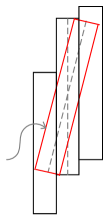
Figure 8. $T^{\delta}_{\xi}$ is covered by the translates of $T^{\delta}_{\xi_{k}}$.

Since $\angle(\xi,\xi_{k})\leq\delta$, there is a $c=c(d)>0$ independent of $\delta$ such that $T^{\delta}_{\xi}$ is covered by a union of at most $c$ many parallel translates of the tube $T^{\delta}_{\xi^{k}}$ ( see Figure 8). Moreover, there are two uniform constants $c_{1},c_{2}$ depending only on $d$ such that

$$c_{1}f^{*}_{\delta}(\xi^{k})\leq f^{*}_{\delta}(\xi)\leq c_{2}f^{*}_{\delta}(\xi^{k}),\quad\forall\angle(\xi,\xi^{k})\leq\delta.$$

Hence (6.1) is bounded up to some constant depending only on $d$ by

$$\sum_{k\in\mathfrak{K}}|f^{*}_{\delta}(\xi^{k})|^{q}\delta^{d-1}.$$ (6.2)

By definition of $f^{*}_{\delta}(\xi^{k})$, there is a tube $T^{\delta}_{k}:=T^{\delta}_{\xi^{k}}(a_{k})$ in direction of $\xi^{k}$ such that

$$\frac{1}{T^{\delta}_{k}}\int_{T^{\delta}_{k}}|f|(y)dy\geq\,\frac{1}{2}\,f^{*}_{\delta}(\xi^{k}).$$

Similarly for any $\xi\in S^{d-1}$ with $\angle(\xi,\xi_{k})\leq\delta$, there is a tube $T^{\delta}_{\xi}(a)$ so that

$$\frac{1}{|T^{\delta}_{\xi}|}\int_{T^{\delta}_{\xi}}|f|(y)dy\geq\,\frac{1}{2}\,f^{*}_{\delta}(\xi).$$

Now, we take a maximal $1-$seperated subset of $\{a_{k}\}_{k\in\mathfrak{K}}$. After relabeling the indices, we may denote this subsequence by $\{a_{j}\}^{J}_{j=1}$ with $J\leq{\rm Card}\mathfrak{K}$. Thus, for any $k\in\mathfrak{K}$, there is some $j\in\{1,\ldots,J\}$ such that $|a_{k}-a_{j}|\leq 1$, and hence $T^{\delta}_{k}\subset B(a_{j},2)$. Based on this observation, we may write

$$\eqref{discretized}\lesssim \sum^{J}_{j=1}\sum_{k:|a_{k}-a_{j}|\leq 1}|\bigl{(}f\chi_{B(a_{j},2)}\bigr{)}^{*}_{\delta}(\xi^{k})|^{q}\delta^{d-1}$$

$$\lesssim \sum^{J}_{j=1}\sum_{k:|a_{k}-a_{j}|\leq 1}\int_{\angle(\xi,\xi^{k})\leq\delta}|\bigl{(}f\chi_{B(a_{j},2)}\bigr{)}^{*}_{\delta}(\xi)|^{q}d\Sigma(\xi)$$

$$\lesssim \sum^{J}_{j=1}\int_{S^{d-1}}|\bigl{(}f\chi_{B(a_{j},2)}\bigr{)}^{*}_{\delta}(\xi)|^{q}d\Sigma(\xi).$$ (6.3)

For $q\geq p$, assume that $\|f^{*}_{\delta}\|_{L^{q}(S^{d-1})}\lesssim_{\varepsilon}\delta^{-\frac{d}{p}+1-\varepsilon}\|f\|_{L^{p}(B(a,2))}$ for all $a\in\mathbb{R}^{d}$. We have by finite overlaps of the balls $\{B(a_{j},2)\}^{J}_{j=1}$ and Minkowski’s inequality

$$\eqref{7.3}\lesssim_{\varepsilon} \delta^{-(\frac{d}{p}-1)q-q\varepsilon}\sum^{J}_{j=1}\Bigl{(}\int_{\mathbb{R}^{d}}|\bigl{(}f\chi_{B(a_{j},2)}\bigr{)}(x)|^{p}dx\Bigr{)}^{\frac{q}{p}}$$

$$\lesssim_{\varepsilon} \delta^{-(\frac{d}{p}-1)q-q\varepsilon}\|f\|^{q}_{L^{p}(\mathbb{R}^{d})}.$$

This yields the same estimate for general $f$.

6.2. The implication of (1.7) to (1.6)

As pointed in [15], Drury [7] had shown the following estimate

$$\|f_{\delta}^{\ast}\|_{L^{d+1}(S^{d-1})}\leq C_{\varepsilon}\delta^{-\frac{d-1}{d+1}-\varepsilon}\|f\|_{L^{\frac{d+1}{2}}(\mathbb{R}^{d})}.$$ (6.4)

We will use this fact as well as the following two estimates

$$\begin{cases}\|f_{\delta}^{\ast}\|_{L^{\infty}(S^{d-1})}\leq\|f\|_{L^{\infty}(\mathbb{R}^{d})},\\ \|f_{\delta}^{\ast}\|_{L^{p,\infty}(S^{d-1})}\leq C_{\varepsilon}\delta^{-\frac{d}{q}+1-\varepsilon}\|f\|_{L^{q,1}(\mathbb{R}^{d})},\leavevmode\nobreak\ p=(d-1)q^{\prime},\end{cases}$$ (6.5)

to derive

$$\|f_{\delta}^{\ast}\|_{L^{p}(S^{d-1})}\leq C_{\varepsilon}\delta^{-\frac{d}{q}+1-\varepsilon}\|f\|_{L^{q}(\mathbb{R}^{d})},\leavevmode\nobreak\ p=(d-1)q^{\prime}.$$ (6.6)

We summarize this as the following lemma.

Lemma 6.1.

Assume $T$ is a sublinear operator, $1\ll A,B<\infty$ and for $p=(d-1)q^{\prime},\leavevmode\nobreak\ q>\frac{d+1}{2},$

$$\|Tf\|_{L^{\infty}(S^{d-1})}\leq \|f\|_{L^{\infty}(\mathbb{R}^{d})},$$ (6.7)

$$\|Tf\|_{L^{d+1}(S^{d-1})}\leq A\|f\|_{L^{\frac{d+1}{2}}(\mathbb{R}^{d})},$$ (6.8)

$$\|Tf\|_{L^{p,\infty}(S^{d-1})}\leq B\|f\|_{L^{q,1}(\mathbb{R}^{d})},$$ (6.9)

then for any $\varepsilon>0$, there holds that

$$\|Tf\|_{L^{p}(S^{d-1})}\leq BA^{\varepsilon}\|f\|_{L^{q}(\mathbb{R}^{d})}.$$ (6.10)

Proof.

We write $f=f_{1}+f_{2}+f_{3}$ with

$$f_{1}=f\chi_{|f|<\frac{\lambda}{3}},\leavevmode\nobreak\ f_{2}=f\chi_{|f|>A^{\alpha}\lambda},\leavevmode\nobreak\ f_{3}=f\chi_{\frac{\lambda}{3}\leq|f|\leq A^{\alpha}\lambda},\leavevmode\nobreak\ \alpha=\frac{2q}{d+1}-1.$$

From the layer cake representation theorem in [10], we obtain

$$\|Tf\|_{L^{p}(S^{d-1})}^{p}= p\int_{0}^{+\infty}\lambda^{p-1}\nu\big{(}\{|Tf|>\lambda\}\big{)}d\lambda$$

$$\leq p\int_{0}^{+\infty}\lambda^{p-1}\Big{[}\nu\big{(}\{|Tf_{1}|>\lambda/3\}\big{)}+\nu\big{(}\{|Tf_{2}|>\lambda/3\}\big{)}+\nu\big{(}\{|Tf_{3}|>\lambda/3\}\big{)}\Big{]}d\lambda$$

$$\triangleq I_{1}+I_{2}+I_{3}.$$

It is easy to see that $I_{1}=0$ since $\nu\big{(}\{|Tf_{1}|>\lambda/3\}\big{)}=0$ by (6.7). To estimate $I_{2}$, we use (6.8) to deduce that

$$\nu\big{(}\{|Tf_{2}|>\lambda/3\}\big{)}\lesssim\frac{A^{d+1}}{\lambda^{d+1}}\|f\|_{L^{\frac{d+1}{2}}}^{d+1}.$$ (6.11)

This together with the trivial estimate

$$\nu\big{(}\{\xi\in S^{d-1}:\leavevmode\nobreak\ |Tf_{2}(\xi)|>\lambda/3\}\big{)}\lesssim 1$$

implies that

$$\nu\big{(}\{|Tf_{2}|>\lambda/3\}\big{)}\lesssim\frac{A^{k}}{\lambda^{k}}\|f\|_{L^{\frac{d+1}{2}}}^{k},\leavevmode\nobreak\ 0\leq k\leq d+1.$$ (6.12)

Hence, we get by Minkowski’s inequality

$$I_{2}= p\int_{0}^{+\infty}\lambda^{p-1}\nu\big{(}\{|Tf_{2}|>\lambda/3\}\big{)}d\lambda\lesssim A^{k}\int_{0}^{+\infty}\lambda^{p-1-k}\|f_{2}\|_{L^{\frac{d+1}{2}}}^{k}d\lambda$$

$$\lesssim A^{k}\bigg{(}\int_{\mathbb{R}^{d}}|f|^{\frac{d+1}{2}}\Big{(}\int_{0}^{+\infty}\lambda^{p-1-k}\chi_{|f|>A^{\alpha}\lambda}d\lambda\Big{)}^{\frac{d+1}{2k}}\bigg{)}^{\frac{2k}{d+1}}$$

$$\lesssim A^{k}A^{-\alpha(p-k)}\Big{(}\int_{\mathbb{R}^{d}}|f|^{\frac{d+1}{2}p}dx\Big{)}^{\frac{2k}{d+1}}\simeq\|f\|_{L^{q}}^{p},$$

where we have used $k=\frac{d+1}{2q}p$ and $\alpha=\frac{2q}{d+1}-1$ in the last step.

Finally, we turn to estimate $I_{3}$. By (6.9) and the characterization of $L^{p,q}$ spaces, one has

$$\nu\big{(}\{|Tf_{3}|>\lambda/3\}\big{)}\leq\frac{B^{p}}{\lambda^{p}}\|f_{3}\|_{L^{q,1}}^{p}\lesssim\frac{B^{p}}{\lambda^{p}}(1+\alpha\log A)^{p-\frac{p}{q}}\|f_{3}\|_{L^{q}}^{p}.$$ (6.13)

Therefore, we estimate by Minkowski’s inequality

$$I_{3}= p\int_{0}^{+\infty}\lambda^{p-1}\nu\big{(}\{|Tf_{3}|>\lambda/3\}\big{)}d\lambda\lesssim B^{p}(1+\alpha\log A)^{p-\frac{p}{q}}\int_{0}^{+\infty}\lambda^{-1}\|f_{3}\|_{L^{q}}^{p}d\lambda$$

$$\lesssim B^{p}(1+\alpha\log A)^{p-\frac{p}{q}}\bigg{(}\int_{\mathbb{R}^{d}}|f|^{q}\Big{(}\int_{0}^{+\infty}\lambda^{-1}\chi_{\frac{\lambda}{3}\leq|f|\leq A^{\alpha}\lambda}d\lambda\Big{)}^{\frac{q}{p}}\bigg{)}^{\frac{p}{q}}$$

$$\lesssim B^{p}(1+\alpha\log A)^{p-\frac{p}{q}}(\log A)\|f\|_{L^{q}}^{p}$$

$$\lesssim B^{p}A^{\varepsilon}\|f\|_{L^{q}}^{p}.$$

Collecting all these estimates on $I_{1},I_{2}$ and $I_{3}$, we obtain

$$\|Tf\|_{L^{p}(S^{d-1})}^{p}\leq I_{1}+I_{2}+I_{3}\lesssim(1+B^{p}A^{\varepsilon})\|f\|_{L^{q}}^{p}.$$

This concludes the lemma.

∎

Acknowledgments

The authors thank the referee and the associated editor for their invaluable comments and suggestions which helped improve the paper greatly. This work is supported in part by the NSF of China under grant No.11171033, No.11231006, and No.11371059. C. Miao is also supported by Beijing Center for Mathematics and Information Interdisciplinary Sciences.

References

- [1] J. Bourgain, Besicovitch type maximal operators and applications to Fourier analysis, Geom. Funct. Anal., Vol. 1, No. 2 (1991) 145-187.
- [2] J. Bourgain, On the dimension of Kakeya sets and related maximal inequalities, Geom. Funct. Anal., Vol. 9 (1999) 256-282.
- [3] J. Bourgain, Harmonic analysis and combinatorics: how much may they contribute to each other?, Mathematics: Frontiers and Perspectives Inernational Mathematical Unions, 13-32(2000)
- [4] J. Bourgain and L. Guth, Bounds on oscillatory integral operators based on multilinear estimates, Geom. Funct. Anal., 21(2011), 1239-1295.
- [5] M. Christ, J. Duoandikoetxea and J. L. Rubio de Francia, Maximal operators assiciated to the Radom transform and the Calderón-Zygmund method of rotations, Duke Math. J. 53 (1986), 189-209.
- [6] A. Cordoba, The Kakeya maximal function and spherical summation multipliers, Amer. J. Math., 99(1977),1-22.
- [7] S. Drury, estimates for the X-ray transform. Illinois J. Math. 27 (1983), 125-129.
- [8] N. Katz and T. Tao. New bounds for Kakeya problems, J.Anal. Math.,87, 231. (2002)
- [9] N. Katz and T. Tao Recent progress on the Kakeya conjecture,
- [10] E. H. Lieb and M. Loss, Analysis. AMS Graduate Studies in Mathematics, Vol. 14 (1987, second edition 2001).
- [11] C. D. Sogge. Concerning Nikodym-type sets in 3-dimensional curved spaces, J. Amer. Math. Soc. 12 (1999), 1-31.
- [12] T. Tao. Edinburg lecture notes on the Kakeya problems.
- [13] T. Tao. The Bochner-Riesz conjecture implies the restriction conjecture, Duke Math J. 96 (1999),363-376.
- [14] T. Tao, A. Vargas and L. Vega, A bilinear approach to the restriction and Kakeya conjectures. J. Amer. Math. Soc. 11 (1998), 967-1000.
- [15] T. Wolff, Recent work connected with the Kakeya problem, Prospects in Mathematics Princeton, NJ, 129-162, AMS, Providence, RI,1999.
- [16] T. Wolff, An improved bound for Kakeya type maximal functions. Revista Math. Iberoamericana 11(1995), 651-674.