One Dimensional Mimicking of Electronic Structure: The Case for Exponentials

Abstract

An exponential interaction is constructed so that one-dimensional atoms and chains of atoms mimic the general behavior of their three-dimensional counterparts. Relative to the more commonly used soft-Coulomb interaction, the exponential greatly diminishes the computational time needed for calculating highly accurate quantities with the density matrix renormalization group. This is due to the use of a small matrix product operator and to exponentially vanishing tails. Furthermore, its more rapid decay closely mimics the screened Coulomb interaction in three dimensions. Choosing parameters to best match earlier calculations, we report results for the one dimensional hydrogen atom, uniform gas, and small atoms and molecules both exactly and in the local density approximation.

I Introduction

The notion that a strong electromagnetic field can be modeled well by a one dimensional (1d) problem dates back to at least 1939 when a calculation by Schiff and Snyder Schiff and Snyder (1939) assigned a potential in the $x$ direction and “integrated out” the transverse degrees of freedom in the $y$ and $z$ directions by averaging over radial wave functions. The resulting interaction has been studied by several others Elliott and Loudon (1960); Knorr and Godby (1992, 1994); Shulenburger et al. (2008, 2009); Casula et al. (2006) including one work by Elliott and Loudon Elliott and Loudon (1960) that approximated the 1d potential, so it can be solved more easily.

Today, the most common approximation for the 1d potentials in a strong electromagnetic field was introduced by Eberly, Su, and Javaninen Eberly et al. (1989) who rewrote the Coulomb interaction $1/\sqrt{x^{2}+y^{2}+z^{2}}$ as $1/\sqrt{x^{2}+a^{2}}$; the $x$ component is allowed to vary independently and the remaining radial term in cylindrical coordinates, $a$, is set to a constant which is determined on a system-by-system basis for the particular application of study to match the ionization energy. This soft-Coulomb interaction has been used in a wide variety of applications requiring a 1d potential Eberly et al. (1989); Law et al. (1991); Joachain et al. (2012); Kreibich et al. (2001); Lein et al. (2000); Chelkowski et al. (1996); Chakravorty and Clementi (1989); Bandrauk (1993); Bandrauk and Wallace (1992). It has many attractive features including the avoidance of the singularity at zero separation while retaining a Rydberg series of excitations Núñez Yépez et al. (2011); Gebremedhin and Weatherford (2014); Carrillo-Bernal et al. (2015). Even when not considering a strong electromagnetic field, the soft-Coulomb interaction has become the choice potential for 1d model systems.

A general use of 1d systems is as a computational laboratory for studying the limitations of electronic structure methods, such as density functional theory (DFT) B. G. Johnson and Pople (1993, 1994a, 1994b); Knorr and Godby (1994); Umrigar and Gonze (1994); Capelle et al. (2003); Magyar and Burke (2004); Capelle et al. (2007); Vieira et al. (2008); Loos and Gill (2009); Helbig et al. (2011); Burke and Wagner (2013a); Wagner et al. (2012); Stoudenmire et al. (2012); Wagner et al. (2013, 2014). A key requirement is that the accuracy of such methods be at least qualitatively similar to their three dimensional (3d) counterparts. Helbig, et. al. Helbig et al. (2011) had already calculated the energy of the uniform electron gas with a soft-Coulomb repulsion, making the construction of the local density approximation (LDA) simple. Recently, some of us Wagner et al. (2012) used Ref. Helbig et al., 2011 to construct benchmark systems with the soft-Coulomb interaction which we used to study DFT approximations Hohenberg and Kohn (1964); Kohn and Sham (1965); Burke (2012); Burke and Wagner (2013b). It was also shown that the model 1d systems closely mimic 3d systems, particularly those with high symmetry. The 1d nature of these systems allows us to use the density matrix renormalization group (DMRG) White (1992) to obtain ground states to numerical precision. DMRG has no sign problem and works well even for strongly correlated 1d systems Snyman (2005). We also apply various DFT approximations to these systems in order to understand how such approximations could be improved, especially when correlations are strong. We have found that our 1d “pseudomolecules” closely mimic the behavior of real 3d molecules in terms of the relative size and type of correlations and also the errors made by DFT approximations Wagner et al. (2012). Conclusions can be drawn from the 1d systems that are relevant to realistic 3d systems, a key advantage over lattice based models. Crucially, in 1d, we can extrapolate to the thermodynamic limit with far less computational cost compared to a similar calculation in 3d Stoudenmire and White (2012).

However, the soft-Coulomb interaction has some drawbacks as a mimic for 3d electronic structure calculations. First, the long $1/|x|$ tail has a bigger effect in 1d than in 3d, making the interaction excessively long ranged. Second, in 3d, the electron-electron interaction induces weak cusps as $\mathbf{r}\rightarrow 0$; the soft-Coulomb induces no cusps at all. While this can be a significant computational advantage with some methods, this precludes using it to study cusp behavior. Third, although the extra cost for treating power-law decaying interactions within DMRG can be made to scale sub-linearly with system size (via a clever fitting approximation McCulloch (2007); Schollwöck (2011)), this cost is still much higher than for a system with strictly local interactions, for example, the Hubbard model Crosswhite et al. (2008).

As an alternative and complement to the soft-Coulomb interaction, we suggest an exponential interaction that addresses each of these weaknesses but whose parameters are chosen to give very similar results. Its tails are weaker, simulating the shorter ranged nature of the Coulomb interaction in 3d if screening is taken into account. The presence of a cusp in the potential more accurately reflects 3d calculations, since a discontinuity in the wavefunction or its derivatives may make convergence more difficult. Finally, the cost for using exponential interactions within DMRG is no more than for using local interactions; in practice this makes DMRG calculations with exponential interactions more than an order of magnitude faster than with soft-Coulomb. Extrapolations to the thermodynamic and continuum limits with exponential interactions also require less computational time.

The primary purpose of this paper is therefore to show in what ways an exponential interaction is preferable to the soft-Coulomb interaction in 1d electronic structure calculations and to provide reference results for such systems. Showing that the soft-Coulomb interaction is well approximated by the exponential would allow for the efficient and fast use of DMRG over QMC methods for 1d systems, so we construct our exponential to also mimic 1d soft-Coulomb calculations and allow for comparison with previous results Luttinger (1963); Haldane (1981, 1983); Hohenberg (1967); Hwang et al. (2007); Gold and Ghazali (1990); Giraud and Combescot (2009); Kivelson et al. (1998); Tanatar (1998); Balents ; Schulz (1990, 1993); Artemenko et al. (2004); Egger and Grabert (1995); Vieira et al. (2008); Lima et al. (2003).

We derive some general analytic forms for the exponential hydrogenic atom in Sec. II and discuss mimicking the soft-Coulomb interaction with $a=1$ in Sec. II.2. Section III summarizes the numerical tools used to find accurate results of the exponential systems. We find the uniform gas energies with DMRG and derive high and low density asymptotic limits in Sec. IV. Finite system calculations and benchmarks for the soft-Coulomb-like exponential interaction are given in Sec. V. The Supplemental Material contains all necessary raw data to reproduce results Baker et al. (2015).

II Hydrogenic Atoms

II.1 General Analytic Expressions

We wish to solve the 1d exponential Hydrogenic atom, with the potential:

$$v_{\rm en}(x)=-Zv_{\mathrm{exp}}(x),\quad v_{\mathrm{exp}}(x)=A\exp(-\kappa|x|).$$ (1)

where $A$ and $\kappa$ characterize the interaction and $Z$ is the ‘charge’ felt by an electron (e) from a nucleus (n). Since the potential is even in $x$, the eigenstates will be even and odd, and we label them $i=0,1,2...$ (alternating even to odd). Writing

$$z(x)=(2\sqrt{2AZ}/\kappa)\,\exp(-\kappa x/2),\quad x\geq 0,$$ (2)

the Schrödinger equation becomes the Bessel equation. The wavefunction solution is a linear combination of $J_{\pm\nu}(z)$, where $\nu^{2}=-8E/\kappa^{2}$, and $J$ is a Bessel function of the first kind. The negative index ($-\nu$) functions diverge as $x\to\infty$, so the wavefunction is proportional to $J_{\nu}(z)$ and the density is

$$n(x)=C^{2}J^{2}_{\nu}(z(|x|))$$ (3)

where $C$ is chosen so that $\int dx\,n(x)=1$.

The eigenvalues, $E$, are determined by spatial symmetry, so that:

$$\left.\frac{d}{dx}J_{\nu}(z)\right|_{z_{0}}=0~{}~{}(\mathrm{even}),~{}~{}~{}~{}~{}~{}J_{\nu}(z_{0})=0~{}~{}(\mathrm{odd}),$$ (4)

with $z_{0}=z(0)$. This condition implies that the eigenfunctions are Bessel functions of non-integer index. Defining $j^{\prime}_{i}(\nu)$ and $j_{i}(\nu)$ to be zeroes of these functions, indexed in order (see e.g., Ref. Abramowitz and Stegun (1965), Sec 9.5), the energy eigenvalues are

$$E_{i}=-\kappa^{2}\,\nu^{2}_{i}(z_{0})/8,~{}~{}~{}~{}i=0,1,2,..$$ (5)

where $\nu_{i}(z_{0})$ satisfies

$$j^{\prime}_{i+1}(\nu_{2i})=z_{0},~{}~{}~{}~{}j_{i}(\nu_{2i-1})=z_{0}.$$ (6)

We found no source where these are generally listed or approximated but they are available in, e.g., Mathematica. One can deduce the critical values of $z_{0}$ at which the number of bound states changes (when $E=0$), since $j^{\prime}_{1}(0)=0$, $j^{\prime}_{2}(0)=3.83171$, $j^{\prime}_{3}(0)=7.01559$, and $j_{1}(0)=2.40483$ and $j_{2}(0)=5.52008$ (Table 9.5 of Ref. Abramowitz and Stegun (1965)).

Unlike a soft-Coulomb potential, cusps appear for the exponential in analogy with 3d Coulomb systems. Rewriting the Schrödinger equation as $\psi^{\prime\prime}/(2\psi)=v_{\rm en}(x)+E$, where $\psi$ is the ground state wavefunction and primes denote derivatives, shows this ratio contains the cusp of the potential at the origin.

II.2 Mimicking Soft-Coulomb Interactions

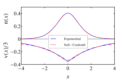
Figure 1: (color online) An exponential interaction with $A=1.071295$ and $\kappa^{-1}=2.385345$ mimics the soft-Coulomb ($a=1$) hydrogen ground-state density very closely.

Now we choose the parameters of our exponential to match closely those of the soft-Coulomb we have previously used in these studies, which has softness parameter $a=1$. In that case, the ground-state energy of the 1d H atom is -0.669778 to $\mu$Ha accuracy Eberly et al. (1989); Wagner et al. (2012); exp , and the width of the ground state density, $\int dx\,n(x)x^{2}$, is 1.191612. We find $A$ and $\kappa$ of $v_{\mathrm{exp}}(x)$ to match these values, yielding:

$$A=1.071295\quad\mathrm{and}\quad\kappa^{-1}=2.385345.$$ (7)

Figure 1 shows the close agreement between the soft-Coulomb and the exponential in both the potential and the density for the 1d H atom. Hereafter, we take these values as defining our choice of exponential interaction.

These values for our hydrogen atom yield $z_{0}=6.983117$, so that it binds exactly four states. Since $z_{0}$ is proportional to ${\sqrt{Z}}$, where $Z$ is the nuclear charge for a hydrogenic atom, a fifth state is just barely bound when $Z=1.00931$. This is a marked difference from the non-interacting soft-Coulomb Loudon (1959) and non-interacting 3d hydrogen Simon (1970) atoms which each bind an infinite number of states.

We then choose the repulsion between electrons to be the same but with opposite sign:

$$v_{\rm ee}(x-x^{\prime})=v_{\mathrm{exp}}(x-x^{\prime}).$$ (8)

Solutions for more than one electron are remarkably similar to the soft-Coulomb under these conditions. For example, both the soft-Coulomb and the exponential bind neutral atoms only up to $Z=4$. We further note that H^- is bound, but H^– is not, for all three cases (exponential, soft-Coulomb, and reality).

III Calculational Details and Notation

DMRG is an exceedingly efficient method for calculating low-energy properties of 1d systems and gives variational energies. For the types of systems considered here, DMRG is able to determine essentially the exact ground state wavefunction Snyman (2005); Schollwöck (2011). DMRG works by iteratively determining the minimal basis of many-body states needed to represent the ground state wavefunction to a given accuracy. For 1d systems, one can reach excellent accuracy by retaining only a few hundred states in the basis. The basis states are gradually improved by projecting the Hamiltonian into the current basis on all but a few lattice sites, then computing the ground state of this partially projected Hamiltonian. The new trial ground state is typically closer to the exact one, making it possible to compute an improved basis.

Our calculations are done in real space on a grid ite . The grid Hamiltonian is chosen to be the extended Hubbard-like model also used in Ref. Wagner et al., 2012 (see Eq. (3) of that work). The electron-electron interaction and external potentials are changed to the exponentials used here. Note that the convention we use to evaluate integrals is to multiply the value of the integrand at each grid point by the grid spacing to match Ref. Wagner et al., 2012. So, for here,

$$\int dx\,f(x)\approx\Delta\sum_{i}f(x_{i})$$ (9)

for some function $f(x)$ and grid spacing $\Delta$. Grid points are indexed by $i$ and span the interval of integration.

Using an exponential interaction within DMRG is very natural since it can be exactly represented by a matrix product operator, the form of the Hamiltonian used in newer DMRG codes McCulloch (2007). In fact, the soft-Coulomb interaction used in Ref. Wagner et al., 2012 was actually represented by fitting it to approximately 25 exponentials Pirvu et al. (2010).

The majority of our focus is on finite systems and we use a finite grid with end points chosen to make the wavefunction negligible. For chains, we place the ends of the grid at the first missing nucleus, although in the case of a single atom or isolated molecule, we will place the boundary sufficiently far from the nuclei to avoid noticeable effects. This can be much nearer to the nuclei than in the soft-Coulomb systems. We always use the convention of placing a grid point on a cusp when possible, to avoid missing any kinetic energy.

In Kohn-Sham (KS) DFT Kohn and Sham (1965), we use density functionals which are defined on the KS system, a non-interacting system that has the same density and energy as the full interacting system. Although, this non-interacting system has a different potential, $v_{s}(x)$, the KS potential. The ground state energy, $E$, of an interacting electron system is the sum of the kinetic energy, $T$, the electron-electron repulsion, $V_{\rm ee}$, and the one-body potential energy, $V$. The ground state energy, $E$, is the minimization in $n$ of the density functional

$$E[n]=T_{\scriptscriptstyle\rm S}[n]+U[n]+V[n]+E_{\scriptscriptstyle\rm XC}[n],$$ (10)

where

$$T_{\scriptscriptstyle\rm S}[n]=\frac{1}{2}\sum_{\sigma}\sum^{N_{\sigma}}_{i=1}\int dx\,\left|\frac{d}{dx}\phi_{i,\sigma}(x)\right|^{2}$$ (11)

is the non-interacting kinetic energy evaluated on the occupied non-interacting KS orbitals, $\phi_{i,\sigma}$, for $N_{\sigma}$ particles of spin $\sigma$. The difference, $T_{\scriptscriptstyle\rm C}=T-T_{\scriptscriptstyle\rm S}$, gives the difference between the interacting and non-interacting kinetic energy. The Hartree integral is defined as

$$U[n]=\frac{1}{2}\iint dx\,dx^{\prime}\,v_{\rm ee}(x-x^{\prime})n(x)n(x^{\prime}).$$ (12)

The one-body potential functional is

$$V[n]=\int dx\,v(x)n(x),$$ (13)

where $v(x)$ is the attraction to the nuclei. Equation 10 defines the exchange-correlation (XC) functional, $E_{\scriptscriptstyle\rm XC}[n]$, which is the sum of the exchange (X) and correlation (C) energies. The exchange energy can be evaluated over the occupied KS orbitals as

$$\begin{split}E_{\scriptscriptstyle\rm X}[n]&=-\frac{1}{2}\sum_{\sigma}\sum^{N_{\sigma}}_{i,j=1}\int dx\int dx^{\prime}\,v_{\rm ee}(x-x^{\prime})\\ &\times\phi^{*}_{i,\sigma}(x)\phi^{*}_{j,\sigma}(x)\phi_{i,\sigma}(x^{\prime})\phi_{j,\sigma}(x^{\prime}),\end{split}$$ (14)

but in practice it is often approximted by an explicity density functional to reduce the computational cost.

IV Uniform Gas

In order to construct and employ the LDA for our exponential repulsion, we must first calculate the exchange-correlation energy of the exponentially repelling uniform gas, expellium.

IV.1 Kinetic, Hartree, and Exchange Energies

These energy components are straightforward and well known, as the single particle states are simply plane waves. The unpolarized, non-interacting kinetic energy per length of a uniform gas is given by Thomas (1927); Fermi (1928); Lieb and Simon (1977)

$$t^{\rm unpol}_{\scriptscriptstyle\rm S}(n)=\pi^{2}n^{3}/24.$$ (15)

The Hartree energy per length of a uniform system with exponential interaction is finite:

$$e_{\scriptscriptstyle\rm H}^{\rm unif}(n)=A\,n^{2}/\kappa.$$ (16)

The exchange energy of the uniform gas was derived in Ref. Elliot et al., 2014, with the energy per length as

$$e^{\rm unpol}_{\scriptscriptstyle\rm X}(n)=A\kappa\left(\ln(1+y^{2})-2y\,\mathrm{arctan}\,y\right)/(2\pi^{2})$$ (17)

where $y=\pi/(2\kappa r_{s})$ where $r_{s}$ is the Wigner-Seitz radius Armiento and Mattsson (2005) in 1d defined as $r_{s}=1/(2n)$ Giuliani and Vignale (2008). The limits for this expression are

$$e_{\scriptscriptstyle\rm X}^{\rm unpol}(n)\rightarrow -An/2,\quad n\rightarrow\infty$$ (18)

$$e_{\scriptscriptstyle\rm X}^{\rm unpol}(n)\rightarrow -An^{2}/(2\kappa),\quad n\rightarrow 0.$$ (19)

Both the exchange and kinetic energies depend separately on the orbitals of each spin, so they satisfy simple spin scaling relation Perdew and Kurth (2003):

$$E_{\scriptscriptstyle\rm X}[n,\zeta]=\frac{1}{2}\left\{E^{\rm unpol}_{\scriptscriptstyle\rm X}[(1+\zeta)n]+E^{\rm unpol}_{\scriptscriptstyle\rm X}[(1-\zeta)n]\right\}$$ (20)

where $\zeta(x)=(n_{\uparrow}(x)-n_{\downarrow}(x))/n(x)$ is the local spin polarization for spin up (down) densities $n_{\uparrow}$ ($n_{\downarrow}$). Applying the relation for $T_{\scriptscriptstyle\rm S}$ yields:

$$t^{\rm unif}_{\scriptscriptstyle\rm S}(n,\zeta)=t_{s}^{\rm unpol}(n)(1+3\zeta^{2})/2$$ (21)

and the exchange energy per length:

$$e^{\rm unif}_{\scriptscriptstyle\rm X}(n,\zeta)=\sum_{\sigma=\pm 1}e^{\rm unpol}_{\scriptscriptstyle\rm X}\Big{(}(1+\sigma\zeta)n\Big{)}/2.$$ (22)

In Fig. 2, we plot the exchange energies per unit length for both the unpolarized and fully polarized cases, comparing with the soft-Coulomb. For $r_{\scriptscriptstyle\rm S}\lesssim 2$, i.e. $n\gtrsim 1/4$, they are very similar, but the exponential vanishes more rapidly in the low density limit. Applying Eq. (19) to Eq. (22) shows $e_{\scriptscriptstyle\rm X}^{\rm unif}$ is independent of $\zeta$ in the high-density limit. Application of Eq. (18) shows $e_{\scriptscriptstyle\rm X}^{\rm unif}(n,\zeta)\rightarrow e_{\scriptscriptstyle\rm X}^{\rm unpol}(n)(1+\zeta^{2})$ as $n\rightarrow 0$.

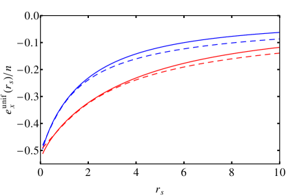
Figure 2: (color online) Exchange energy densities per particle of the uniform gas for the exponential (solid lines), both unpolarized (blue) and fully polarized (red). Dashed lines show soft-Coulomb results.

IV.2 Correlation Energy

While we can determine the exchange energy of the uniform gas analytically, for correlation we cannot. We first determine the high and low density limits and connect them with a Padé approximation.

IV.3 High Density Limit

In the high-density uniform gas, the RPA solution becomes exact e.g. and Pines (1958); Gell-Mann and Brueckner (1957); Li et al. (1992); Sarma and Hwang (1996); Li and Sarma (1991); Fetter and Walecka (1971); Giuliani and Vignale (2005); Fetter and Walecka (1971); Ziman (1972); Langreth and Perdew (1977); Rajagopal and Kimball (1977). Casula, et. al. Casula et al. (2006) have derived a criteria for the RPA limit which for 1d systems gives $e_{\scriptscriptstyle\rm C}=-\Upsilon r_{\scriptscriptstyle\rm S}/\pi^{4}$ where $\Upsilon=\int_{0}^{\infty}dq\,q\tilde{v}_{\rm ee}^{2}(q)$ for the Fourier transform, $\tilde{v}_{\rm ee}(q)=2A\kappa/(\kappa^{2}+q^{2})$ Casula et al. (2006); Shulenburger et al. (2008, 2009); Helbig et al. (2011). Thus,

$$e_{\scriptscriptstyle\rm C}^{\mathrm{RPA}}(n)=\begin{cases}-2A^{2}r_{s}/\pi^{4}&\mathrm{unpolarized},\\ -A^{2}r_{s}/(4\pi^{4})&\mathrm{polarized}.\end{cases}$$ (23)

Note that these expressions for the exponential $e^{\mathrm{RPA}}_{\scriptscriptstyle\rm C}$ are identical to the $e^{\mathrm{RPA}}_{\scriptscriptstyle\rm C}$ of the soft-Coulomb interaction if $A=1$ and so differ by less than 15% here Helbig et al. (2011).

IV.4 Low Density Limit

To determine the low density limit of the correlation, we may work in the limit of a Wigner crystal Wigner (1932). This phase occurs because the kinetic energy becomes less than the interaction energy for low densities. The strictly correlated electron limit M. Seidl and Levy (1999); Seidl et al. (2007); Magyar and Burke (2004) is the exact limit of the low density electron gas Seidl et al. (2000); Giuliani and Vignale (2008). For strictly correlated electrons, each electron sits some multiple of $2r_{\scriptscriptstyle\rm S}$ away from any other. For short-ranged interactions, such as the exponential, the potential energy must decay exponentially with $r_{\scriptscriptstyle\rm S}$, so that $E_{\scriptscriptstyle\rm XC}=-U$, regardless of spin polarization Perdew and Kurth (2003). The actual form of the correlation energy $e_{\scriptscriptstyle\rm C}$, however, will depend on the polarization, because the exchange energy $e_{\scriptscriptstyle\rm X}$ does. For a spin-unpolarized system, using Eq. (19), we find $e_{\scriptscriptstyle\rm X}(n)=e_{\scriptscriptstyle\rm C}(n)=-An^{2}/(2\kappa)$ in the low-density gas limit. After spin-scaling exchange, we obtain the low-density limit $e_{\scriptscriptstyle\rm X}^{\rm pol}(n)=-An^{2}/\kappa$, and this quantity already cancels the Hartree energy! Therefore the correlation energy for spin-polarized electrons must decay more rapidly than $n^{2}$ as $n\rightarrow 0$.

IV.5 Correlation Energy Calculations

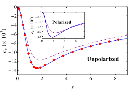
Figure 3: (color online) Correlation energy densities of the uniform gas from DMRG calculations. Solid lines are parametrization of Eq. (24), red dots are calculated, and dashed lines are for the soft-Coulomb Helbig et al. (2011).

The uniform gas correlation energy was found from a sequence of DMRG calculations in boxes of increasing length, $L$, in which the average density is kept fixed. Grid errors become more pronounced in these systems compared with soft-Coulomb interactions because there is no way to ensure a grid point will always lie on the wave function’s cusp. Hence, a very fine grid spacing was necessary to converge the points. As the density increases, finer and finer grids were necessary, down to a practical limit of $\Delta=0.008$. Energies for different box sizes were fit to a parabola in $1/L$ and the limit of $L\rightarrow\infty$ extracted. The various energy components of Sec. IV.1 were then subtracted to find $e_{\scriptscriptstyle\rm C}$ to make the dots in Fig. 3. For partially polarized gases, we used the same procedure as for the unpolarized case except that each box contained various values of $\zeta$ for each $L$ used in the limit. Evaluating several partially polarized systems, we found that the correlation energy was very nearly parabolic in $\zeta$ at several different densities.

IV.6 Padé Approximation

Considering the asymptotic limits of the correlation energy, the full approximation that allows us to accurately fit the data is

$$e^{\rm unif}_{\scriptscriptstyle\rm C}=\frac{-A\kappa y^{2}/\pi^{2}}{\alpha+\beta\sqrt{y}+\gamma y+\delta y^{3/2}+\eta y^{2}+\sigma y^{5/2}+\nu\frac{\pi\kappa^{2}}{A}y^{3}}.$$ (24)

where $y$ was defined above and the fitting parameters are defined for this specific choice of $A$ and $\kappa$ only. The parameters optimized by fitting DMRG uniform gas data are given in Table 1, and the resulting fits are shown in Fig. 3. Although we know at full polarization $e_{\scriptscriptstyle\rm C}$ should decay more rapidly than $n^{2}$ in the low density limit, we do not know how much more rapidly, so we use the same form as the unpolarized case. This fit is accurate and the coefficient of $n^{2}$ is about 1% that of the unpolarized one. Finally, we approximate the $\zeta$ dependence as

$$e_{c}(n,\zeta)=e_{c}^{\rm unpol}(n)+\zeta^{2}\Big{(}e_{c}^{\rm pol}(n)-e_{c}^{\rm unpol}(n)\Big{)},$$ (25)

as justified in the previous section.

	$\alpha$	$\beta$	$\gamma$	$\delta$	$\eta$	$\sigma$
$e^{\rm unpol}_{c}$	2	-1.00077	6.26099	-11.9041	9.62614	-1.48334
$e^{\rm pol}_{c}$	180.891	-541.124	651.615	-356.504	88.0733	-4.32708

Table 1: Fitting parameters for the correlation energy in Eq. (24). The parameter $\nu=1$ (unpolarized) or 8 (polarized).

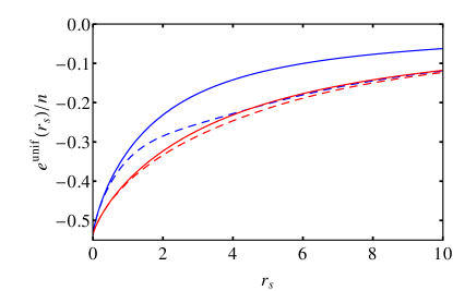
Figure 4: (color online) XC energy per particle, $e_{\scriptscriptstyle\rm XC}/n$ (dashed), for the unpolarized (blue) and fully polarized (red). Solid lines are $e_{\scriptscriptstyle\rm X}/n$ only.

In Fig. 4, we show the combined XC energies (solid) for the unpolarized (blue) and polarized gases (red). Dashed lines are for exchange alone. Correlation is a much smaller effect in the fully spin-polarized gas.

V Finite Systems

V.1 Atomic Energies

$N_{\text{e}}$	Symb.	$E^{\mathrm{HF}}$	$E$	$E_{\scriptscriptstyle\rm C}^{\mathrm{QC}}$	$T$	$V$	$V_{\rm ee}$	$T_{s}$	$U$	$E_{\scriptscriptstyle\rm XC}$	$E_{\scriptscriptstyle\rm X}$	$E_{\scriptscriptstyle\rm C}$	$T_{\scriptscriptstyle\rm C}$	$E^{\rm LDA}$	$E^{\rm LDA}_{\scriptscriptstyle\rm X}$	$E^{\rm LDA}_{\scriptscriptstyle\rm C}$
1	H	-0.670	-0.670	0	0.111	-0.781	0	0.111	0.345	-0.345	-0.345	0	0	-0.643	-0.305	-0.009
	He+	-1.482	-1.482	0	0.190	-1.672	0	0.190	0.379	-0.379	-0.379	0	0	-1.449	-0.337	-0.007
	Li++	-2.334	-2.334	0	0.259	-2.593	0	0.259	0.397	-0.397	-0.397	0	0	-2.298	-0.355	-0.006
	Be3+	-3.208	-3.208	0	0.321	-3.529	0	0.321	0.408	-0.408	-0.408	0	0	-3.171	-0.366	-0.005
2	H-	-0.694	-0.737	-0.044	0.114	-1.311	0.460	0.081	1.070	-0.586	-0.535	-0.051	0.050	-0.711	-0.520	-0.073
	He	-2.223	-2.237	-0.014	0.286	-3.212	0.690	0.273	1.432	-0.730	-0.716	-0.014	0.013	-2.196	-0.633	-0.050
	Li+	-3.884	-3.892	-0.008	0.433	-5.080	0.755	0.426	1.541	-0.779	-0.770	-0.009	0.007	-3.842	-0.686	-0.039
	Be++	-5.606	-5.611	-0.005	0.564	-6.967	0.792	0.559	1.602	-0.806	-0.801	-0.005	0.005	-5.556	-0.715	-0.034
3	Li	-4.199	-4.215	-0.016	0.628	-6.490	1.647	0.614	2.751	-1.089	-1.072	-0.017	0.014	-4.181	-0.999	-0.045
	Be+	-6.447	-6.457	-0.010	0.910	-9.225	1.858	0.900	3.029	-1.161	-1.150	-0.011	0.010	-6.411	-1.074	-0.035
4	Be	-6.756	-6.809	-0.053	1.118	-11.115	3.188	1.077	4.710	-1.481	-1.421	-0.060	0.041	-6.784	-1.371	-0.080

Table 2: Energy components for several systems as calculated by DMRG to 1 mHa accuracy. Chemical symbols H, He, Li, and Be imply single atomic potentials of $Z=1,2,3,$ and 4, respectively. All LDA calculations are self-consistent, except H^-, which is unbound, so we evaluate $E_{\scriptscriptstyle\rm XC}^{\rm LDA}$ on the exact density Kim et al. (2013). These values are very similar to those of the soft-Coulomb Wagner et al. (2012).

We now refer to several tables that contain the information from several different systems as determined by the methods of the previous sections. To construct the LDA, $E_{\scriptscriptstyle\rm XC}^{\rm LDA}$ is constructed from Eqs. (17) and (25). In practice, we always use spin-DFT, and the local spin density approximation (LSDA). The plot of $e^{\rm unif}_{\scriptscriptstyle\rm XC}(r_{\scriptscriptstyle\rm S},\zeta)$ is very similar to those of the soft-Coulomb (see Fig. 2 of Ref. Wagner et al., 2012).

Table 2 contains many energy components for all 1d atoms and ions up to $Z=4$. The total energies are accurate to within 1 mHa. The first approximation in quantum chemistry is the Hartree-Fock (HF), and its error is the (quantum chemical) correlation energy, $E_{\scriptscriptstyle\rm C}^{\mathrm{QC}}$. As required, this is always negative and is typically a very small fraction of $|E|$. Unlike real atoms and ions, for fixed particle number $N$, $E_{\scriptscriptstyle\rm C}\rightarrow 0$ as $Z\rightarrow\infty$, not a constant S.J. Chakravorty and Fischer (1993).

The next three columns show the breakdown of $E$ into its various components. The magnitude of $|V|$ is much greater than the other two. Unlike 3d Coulomb systems, there is no virial theorem relating $E$ and $-T$, for example Levine (2008). Here the kinetic energies are much smaller than $|E|$, just as for the soft-Coulomb Wagner et al. (2012). In the following three columns we give the KS components of the energy. These were extracted by finding the exact $v_{\scriptscriptstyle\rm S}(x)$ from $n(x)$ Wagner et al. (2014), and constructing the exact KS quantities Kohn and Sham (1965). Unlike 3d Coulomb reality, $T_{\scriptscriptstyle\rm S}$ is smaller in magnitude than $|E_{\scriptscriptstyle\rm XC}|$. But just like in 3d Coulomb reality, both $T_{\scriptscriptstyle\rm S}$ and $E_{\scriptscriptstyle\rm XC}$ always grow with $Z$ if $N$ is fixed, with $N$ if $Z$ is fixed, or with $Z$ for $Z=N$ Burke (2007).

The next set of columns break $E_{\scriptscriptstyle\rm XC}$ into its components: $E_{\scriptscriptstyle\rm X}$, $E_{\scriptscriptstyle\rm C}$, and $T_{\scriptscriptstyle\rm C}$. The correlation energy is negative everywhere and is slightly larger in magnitude than $|E_{\scriptscriptstyle\rm C}^{\mathrm{QC}}|$ as required Petersilka and Gross (1996). We also see $T_{\scriptscriptstyle\rm C}$ is very close to $-E_{\scriptscriptstyle\rm C}$ everywhere, a sign of weak correlation Burke (2006), which is the same as in 3d Coulomb atoms and ions. We also report self-consistent LDA energies and the XC components. All LDA energies are insufficiently negative. For $N=1$, self-interaction error occurs and $E_{\scriptscriptstyle\rm XC}^{\rm LDA}$ is not quite $-U$. Just as for reality, LDA exchange consistently underestimates the magnitude of $E_{\scriptscriptstyle\rm X}$, while $E_{\scriptscriptstyle\rm C}^{\rm LDA}$ overestimates, producing the well-known cancellation of errors in $E_{\scriptscriptstyle\rm XC}^{\rm LDA}$.

$N_{\text{e}}$	Symb.	LDA		HF		Exact
		$-\epsilon_{\scriptscriptstyle\rm H}$	I	$-\epsilon_{\scriptscriptstyle\rm H}$	I	I$=-\epsilon_{\scriptscriptstyle\rm H}$
1	H	0.412	0.643	0.670	0.670	0.670
2	H-	–	0.062	0.058	0.024	0.068
	He	0.478	0.714	0.750	0.741	0.755
	Li+	1.238	1.508	1.556	1.550	1.558
	Be++	2.061	2.348	2.402	2.403	2.403
3	Li	0.182	0.339	0.327	0.315	0.323
	Be+	0.643	0.855	0.850	0.836	0.846
4	Be	0.183	0.373	0.327	0.309	0.331

Table 3: Highest occupied eigenvalues $(\epsilon_{\scriptscriptstyle\rm H})$ and total energy differences ($I$) for several atoms and ion, both exactly and approximately.

We close the section on atoms with details of eigenvalues. It is long known that Almbladh and Von Barth (1985), for the exact KS potential, the highest occupied eigenvalue is at $-I$, the ionization energy, but that this condition is violated by approximation. In Table 3, we list $-\epsilon_{\scriptscriptstyle\rm H}$ and $I$ for several atoms and ions exactly, in HF and in LDA. Koopman first argued Koopmans (1934) that $-\epsilon_{\scriptscriptstyle\rm H}$ should be a good approximation to $I$ in HF, and we see that, just as in reality, it is a better approximation to $I$ than $I^{\mathrm{HF}}$, from total energy differences. On the other hand, our 1d LDA exhibits the same well-known failure of real LDA: its KS potential is far too shallow, so that $\epsilon_{\scriptscriptstyle\rm H}^{\rm LDA}$ is above $\epsilon_{\scriptscriptstyle\rm H}$ by a significant amount (up to 10 eV).

V.2 Molecular Dissociation

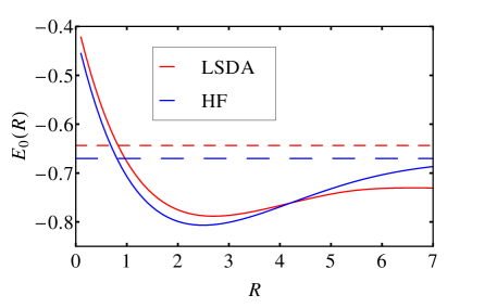
Figure 5: (color online) Molecular dissociation for H${}_{2}^{+}$ for LSDA and HF. Dashed lines indicate the energy of a single H atom. Results are in close agreement with the soft-Coulomb interaction (see Fig. 1 of Ref. Helbig et al., 2011 and Fig. 8 of Ref. Wagner et al., 2012). LSDA has the well known failure of not dissociating to the correct limit Burke (2007).

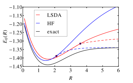
Figure 6: (color online) Molecular dissociation for H₂ with dots denoting the Coulson-Fischer points. Curves are shown for the exact case; also shown are restricted (solid) and unrestricted (dashed) LSDA and HF.

Next we consider 1d molecules with an exponential interaction. The behavior is almost identical to that of the soft-Coulomb documented in Ref. Wagner et al., 2012. For H${}_{2}^{+}$, in Fig. 5, HF is exact, and $E_{0}^{\mathrm{LSDA}}(R\rightarrow\infty)$ does not tend to $E_{0}^{\mathrm{LSDA}}(\mathrm{H})$ because of a large self-interaction error Cohen et al. (2008).

For H₂, in Fig. 6, the exact curve is calculated with DMRG, which has no problems whatsoever with stretching the bond (and can even break triple bonds Chan and Head-Gordon (2002)). But HF, restricted to a singlet, tends to the wrong limit as $R\rightarrow\infty$, while unrestricted HF goes to a lower energy beyond the Coulson-Fischer Coulson and Fischer (1949) point ($R=2.1$) and dissociates to the correct energy $(2E(H))$ but the wrong spin symmetry Perdew et al. (1995). The same qualitative behavior occurs for LSDA at $R=3.6$. These results are almost identical to those with soft-Coulomb interactions (except $R=3.4$ for the soft-Coulomb LSDA Coulson-Fischer point), and qualitatively the same as 3D.

For reference purposes, we also report equilibrium properties of H₂ and H${}_{2}^{+}$ in Table 4. HF is exact for H${}_{2}^{+}$, but underbinds H₂, shortens its bond, and yields too large a vibrational frequency, just as in 3d. Overall, LSDA results are substantially more accurate. LSDA overbinds, yields slightly (to less than 1%) too large a bond, and only slightly overestimates vibrational frequencies, just as in reality. Vibrational frequencies, $\omega$, are chosen to fit the function $E_{0}+\omega^{2}(r-R_{0})^{2}/2$.

	H${}_{2}^{+}$		H2
quantity	LSDA	exact	HF	LSDA	exact
$D_{\text{e}}$ (eV)	3.94	3.72	2.04	3.25	2.74
$R_{0}$ (bohr)	2.70	2.50	1.45	1.60	1.56
$\omega$ ($\times 10^{3}$ cm-1)	2.03	2.32	3.91	3.52	3.40

Table 4: Electronic well depth $D_{\text{e}}$ (calculated relative to well-separated unrestricted atoms), equilibrium bond radius $R_{0}$, and vibrational frequency $\omega$ for the H${}_{2}^{+}$ and H₂ molecules.

V.3 Relative Advantages

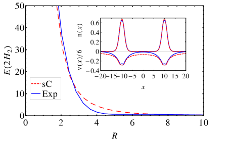
Figure 7: (color online) Binding energy curves for two H₂ molecules a distance $R$ apart (measured between the innermost atoms), demonstrating the much slower decay of the soft-Coulomb. We subtracted off the asymptote of the binding curve so that the curves tend to zero. The inset shows the soft-Coulomb potentials from the two H₂ atoms have a substantial overlap even at $R=18$ while the exponential does not.

To illustrate the effective shorter range of the exponential relative to a soft-Coulomb, Fig. 7 shows the exact binding energy of two H₂ molecules (with bond lengths set to their equilibrium values for each type of interaction) as a function of the separation between closest nuclei. These closed shell molecules do not bind with either interaction, but the soft-Coulomb energy decays far more slowly to its value at $\infty$.

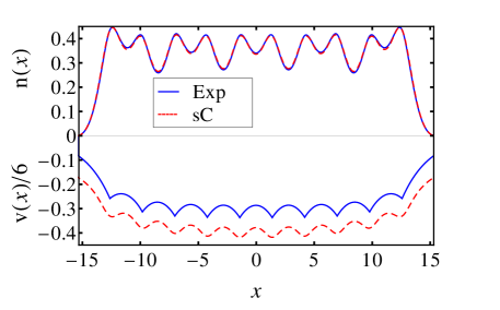
Figure 8: (color online) The density of an H₁₀ chain with $R=2.8$ with exponential and soft-Coulomb interactions.

Finally, we give an example of the much lower computational cost of the exponential in DMRG over that of the soft-Coulomb due to the reasons discussed in Sec. I. In Fig. 8, we plot the densities and potentials for a 10-atom H chain with separations $R=2.8$. The densities are sufficiently similar for all practical purposes (but not the potentials) while the computational time per DMRG sweep was about 4 times longer for the soft-Coulomb. With increasing interatomic distance, Fig. 9 shows a decreased wall time of more than a factor of 20 for calculating larger separations.

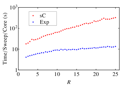
Figure 9: (color online) The exponential performs sweeps in DMRG much faster, leading to a greatly reduced computational time. Here we show the cost of the H₁₀ of Fig. 8 as a function of interatomic separation. The number of many body states is fixed at 30 for 10 sweeps and each system has 1161 grid points. The maximum truncation error in each sweep is $\sim 10^{-8}$.

VI Conclusion

We have introduced an exponential interaction that allows us to mimic many features of real electronic structure with 1d systems. Using the exponential in place of the more standard soft-Coulomb interaction not only improves the computational time of DMRG , but it also allows faster convergence for other calculations due to its fast decay and local nature. To facilitate comparison with existing calculations, we choose the parameters in the exponential to best match a soft-Coulomb potential. A parameterization for the LDA is given by calculating and fitting to uniform gas data.

VII Acknowledgments

This work was supported by the U.S. Department of Energy, Office of Science, Basic Energy Sciences under award #DE-SC008696. T.E.B. also thanks the gracious support of the Pat Beckman Memorial Scholarship from the Orange County Chapter of the Achievement Rewards for College Scientists Foundation.

References

- Schiff and Snyder (1939) LI Schiff and H Snyder, “Theory of the quadratic zeeman effect,” Physical Review 55, 59 (1939).
- Elliott and Loudon (1960) RJ Elliott and R Loudon, “Theory of the absorption edge in semiconductors in a high magnetic field,” Journal of Physics and Chemistry of Solids 15, 196–207 (1960).
- Knorr and Godby (1992) W Knorr and RW Godby, “Investigating exact density-functional theory of a model semiconductor,” Physical review letters 68, 639 (1992).
- Knorr and Godby (1994) W Knorr and RW Godby, “Quantum monte carlo study of density-functional theory for a semiconducting wire,” Physical Review B 50, 1779 (1994).
- Shulenburger et al. (2008) Luke Shulenburger, Michele Casula, Gaetano Senatore, and Richard M Martin, “Correlation effects in quasi-one-dimensional quantum wires,” Physical Review B 78, 165303 (2008).
- Shulenburger et al. (2009) Luke Shulenburger, Michele Casula, Gaetano Senatore, and Richard M Martin, “Spin resolved energy parametrization of a quasi-one-dimensional electron gas,” Journal of Physics A: Mathematical and Theoretical 42, 214021 (2009).
- Casula et al. (2006) Michele Casula, Sandro Sorella, and Gaetano Senatore, “Ground state properties of the one-dimensional coulomb gas using the lattice regularized diffusion monte carlo method,” Physical Review B 74, 245427 (2006).
- Eberly et al. (1989) Joseph H Eberly, Q Su, and Juha Javanainen, “High-order harmonic production in multiphoton ionization,” JOSA B 6, 1289–1298 (1989).
- Law et al. (1991) CK Law, Q Su, and JH Eberly, “Stabilization of a model atom undergoing three-photon ionization,” Physical Review A 44, 7844 (1991).
- Joachain et al. (2012) Charles Jean Joachain, Niels J Kylstra, and Robert M Potvliege, Atoms in intense laser fields (Cambridge University Press, 2012).
- Kreibich et al. (2001) Thomas Kreibich, Manfred Lein, Volker Engel, and EKU Gross, “Even-harmonic generation due to beyond-born-oppenheimer dynamics,” Physical review letters 87, 103901 (2001).
- Lein et al. (2000) M Lein, EKU Gross, and V Engel, “On the mechanism of strong-field double photoionization in the helium atom,” Journal of Physics B: Atomic, Molecular and Optical Physics 33, 433 (2000).
- Chelkowski et al. (1996) Szczepan Chelkowski, André Conjusteau, Tao Zuo, and André D Bandrauk, “Dissociative ionization of h 2+ in an intense laser field: Charge-resonance-enhanced ionization, coulomb explosion, and harmonic generation at 600 nm,” Physical Review A 54, 3235 (1996).
- Chakravorty and Clementi (1989) Subhas Chakravorty and Enrico Clementi, “Soft coulomb hole for the hartree-fock model to estimate atomic correlation energies,” Phys. Rev. A 39, 2290–2296 (1989).
- Bandrauk (1993) André D Bandrauk, Molecules in laser fields (CRC Press, 1993).
- Bandrauk and Wallace (1992) André D Bandrauk and Stephen C Wallace, Coherence phenomena in atoms and molecules in laser fields, Vol. 287 (Plenum Publishing Corporation, 1992).
- Núñez Yépez et al. (2011) H. N. Núñez Yépez, A. L. Salas-Brito, and Didier A. Solis, “Quantum solution for the one-dimensional coulomb problem,” Phys. Rev. A 83, 064101 (2011).
- Gebremedhin and Weatherford (2014) Daniel H Gebremedhin and Charles A Weatherford, “Calculations for the one-dimensional soft coulomb problem and the hard coulomb limit,” Physical Review E 89, 053319 (2014).
- Carrillo-Bernal et al. (2015) M. A. Carrillo-Bernal, H. N. Núñez Yépez, A. L. Salas-Brito, and Didier A. Solis, “Comment on “calculations for the one-dimensional soft coulomb problem and the hard coulomb limit”,” Phys. Rev. E 91, 027301 (2015).
- B. G. Johnson and Pople (1993) P. M. W. Gill B. G. Johnson and J. A. Pople, J. Chem. Phys. 98, 5612 (1993).
- B. G. Johnson and Pople (1994a) P. M. W. Gill B. G. Johnson and J. A. Pople, “A rotationally invariant procedure for density functional calculations,” Chem. Phys. Lett. 220, 377 (1994a).
- B. G. Johnson and Pople (1994b) P. M. W. Gill B. G. Johnson, C. A. Gonzales and J. A. Pople, “A density functional study of the simplest hydrogen abstraction reaction. effect of self-interaction correction,” Chem. Phys. Lett. 221, 100 (1994b).
- Umrigar and Gonze (1994) C. J. Umrigar and Xavier Gonze, “Accurate exchange-correlation potentials and total-energy components for the helium isoelectronic series,” Phys. Rev. A 50, 3827–3837 (1994).
- Capelle et al. (2003) K Capelle, NA Lima, MF Silva, and LN Oliveira, “Density-functional theory for the hubbard model: numerical results for the luttinger liquid and the mott insulator,” in The Fundamentals of Electron Density, Density Matrix and Density Functional Theory in Atoms, Molecules and the Solid State (Springer, 2003) pp. 145–168.
- Magyar and Burke (2004) R.J. Magyar and Kieron Burke, “Density-functional theory in one dimension for contact-interacting fermions,” Phys. Rev. A 70, 032508 (2004).
- Capelle et al. (2007) Klaus Capelle, Magnus Borgh, Kimmo Kärkkäinen, and SM Reimann, “Energy gaps and interaction blockade in confined quantum systems,” Physical review letters 99, 010402 (2007).
- Vieira et al. (2008) Daniel Vieira, Henrique JP Freire, VL Campo Jr, and Klaus Capelle, “Friedel oscillations in one-dimensional metals: From luttinger’s theorem to the luttinger liquid,” Journal of Magnetism and Magnetic Materials 320, e418–e420 (2008).
- Loos and Gill (2009) Pierre-Francois Loos and Peter M. W. Gill, “Two electrons on a hypersphere: A quasiexactly solvable model,” Phys. Rev. Lett. 103, 123008 (2009).
- Helbig et al. (2011) N Helbig, Johanna I Fuks, M Casula, Matthieu J Verstraete, Miguel AL Marques, IV Tokatly, and A Rubio, “Density functional theory beyond the linear regime: Validating an adiabatic local density approximation,” Physical Review A 83, 032503 (2011).
- Burke and Wagner (2013a) Kieron Burke and Lucas O. Wagner, “DFT in a nutshell,” International Journal of Quantum Chemistry 113, 96–101 (2013a).
- Wagner et al. (2012) Lucas O. Wagner, E.M. Stoudenmire, Kieron Burke, and Steven R. White, “Reference electronic structure calculations in one dimension,” Phys. Chem. Chem. Phys. 14, 8581 – 8590 (2012).
- Stoudenmire et al. (2012) E. M. Stoudenmire, Lucas O. Wagner, Steven R. White, and Kieron Burke, “One-dimensional continuum electronic structure with the density-matrix renormalization group and its implications for density-functional theory,” Phys. Rev. Lett. 109, 056402 (2012).
- Wagner et al. (2013) Lucas O. Wagner, E. M. Stoudenmire, Kieron Burke, and Steven R. White, “Guaranteed convergence of the kohn-sham equations,” Phys. Rev. Lett. 111, 093003 (2013).
- Wagner et al. (2014) Lucas O. Wagner, Thomas E. Baker, E.M. Stoudenmire, Kieron Burke, and Steven R. White, “Kohn-sham calculations with the exact functional,” Phys. Rev. B 90, 045109 (2014).
- Hohenberg and Kohn (1964) P. Hohenberg and W. Kohn, “Inhomogeneous electron gas,” Phys. Rev. 136, B864–B871 (1964).
- Kohn and Sham (1965) W. Kohn and L. J. Sham, “Self-consistent equations including exchange and correlation effects,” Phys. Rev. 140, A1133–A1138 (1965).
- Burke (2012) K. Burke, “Perspective on density functional theory,” J. Chem. Phys. 136 (2012).
- Burke and Wagner (2013b) Kieron Burke and Lucas O. Wagner, “Dft in a nutshell,” Int. J. Quant. Chem. 113, 96–101 (2013b).
- White (1992) Steven R. White, “Density matrix formulation for quantum renormalization groups,” Phys. Rev. Lett. 69, 2863–2866 (1992).
- Snyman (2005) Jan A. Snyman, Practical Mathematical Optimization (Springer, New York, 2005).
- Stoudenmire and White (2012) E M Stoudenmire and Steven R White, “Studying two-dimensional systems with the density matrix renormalization group,” Annual Review of Condensed Matter Physics 111 (2012).
- McCulloch (2007) Ian P McCulloch, “From density-matrix renormalization group to matrix product states,” Journal of Statistical Mechanics: Theory and Experiment 2007, P10014 (2007).
- Schollwöck (2011) Ulrich Schollwöck, “The density-matrix renormalization group in the age of matrix product states,” Annals of Physics 326, 96 – 192 (2011), january 2011 Special Issue.
- Crosswhite et al. (2008) Gregory M. Crosswhite, A. C. Doherty, and Guifré Vidal, “Applying matrix product operators to model systems with long-range interactions,” Phys. Rev. B 78, 035116 (2008).
- Luttinger (1963) JM Luttinger, “An exactly soluble model of a many-fermion system,” Journal of Mathematical Physics 4, 1154–1162 (1963).
- Haldane (1981) FDM Haldane, “Effective harmonic-fluid approach to low-energy properties of one-dimensional quantum fluids,” Physical Review Letters 47, 1840 (1981).
- Haldane (1983) F Duncan M Haldane, “Continuum dynamics of the 1-d heisenberg antiferromagnet: identification with the o (3) nonlinear sigma model,” Physics Letters A 93, 464–468 (1983).
- Hohenberg (1967) PC Hohenberg, “Existence of long-range order in one and two dimensions,” Physical Review 158, 383 (1967).
- Hwang et al. (2007) CG Hwang, SY Shin, and JW Chung, “Plasmon excitation observed in quasi one-dimensional nanowires,” in Journal of Physics: Conference Series, Vol. 61 (IOP Publishing, 2007) p. 454.
- Gold and Ghazali (1990) A Gold and A Ghazali, “Analytical results for semiconductor quantum-well wire: Plasmons, shallow impurity states, and mobility,” Physical Review B 41, 7626 (1990).
- Giraud and Combescot (2009) S Giraud and R Combescot, “Highly polarized fermi gases: One-dimensional case,” Physical Review A 79, 043615 (2009).
- Kivelson et al. (1998) Steven A Kivelson, Eduardo Fradkin, and Victor J Emery, “Electronic liquid-crystal phases of a doped mott insulator,” Nature 393, 550–553 (1998).
- Tanatar (1998) B Tanatar, “Many-body effects in a two-component, one-dimensional electron gas with repulsive, short-range interactions,” Physics Letters A 239, 300–306 (1998).
- (54) Leon Balents, “Notes by l. balents for k. burke,” .
- Schulz (1990) H. Schulz, “Correlation exponents and the metal-insulator transition in the one-dimensional hubbard model,” Phys. Rev. Lett. 64, 2831–2834 (1990).
- Schulz (1993) HJ Schulz, “Wigner crystal in one dimension,” Physical review letters 71, 1864 (1993).
- Artemenko et al. (2004) SN Artemenko, Gao Xianlong, and W Wonneberger, “Friedel oscillations in a gas of interacting one-dimensional fermionic atoms confined in a harmonic trap,” Journal of Physics B: Atomic, Molecular and Optical Physics 37, S49 (2004).
- Egger and Grabert (1995) Reinhold Egger and Hermann Grabert, “Friedel oscillations for interacting fermions in one dimension,” Physical review letters 75, 3505 (1995).
- Lima et al. (2003) NA Lima, MF Silva, LN Oliveira, and K Capelle, “Density functionals not based on the electron gas: local-density approximation for a luttinger liquid,” Physical review letters 90, 146402 (2003).
- Baker et al. (2015) Thomas E Baker, E Miles Stoudenmire, Lucas O Wagner, Kieron Burke, and Steven R White, “One-dimensional mimicking of electronic structure: The case for exponentials,” Physical Review B 91, 235141 (2015).
- Abramowitz and Stegun (1965) M. Abramowitz and I.A. Stegun, Handbook of Mathematical Functions: With Formulas, Graphs, and Mathematical Tables, Applied mathematics series (Dover Publications, 1965).
- (62) “References Eberly et al., 1989 and Wagner et al., 2012 gives the ground state energy as -0.669777, but a truncation in the variables and change our energy slightly.” .
- Loudon (1959) Rodney Loudon, “One-dimensional hydrogen atom,” American Journal of Physics 27, 649–655 (1959).
- Simon (1970) Barry Simon, Infinitude or finiteness of the number of bound states of an N-body quantum system. I., Tech. Rep. (Princeton Univ., NJ, 1970).
- (65) “Calculations were performed using the itensor library: http://itensor.org/,” .
- Pirvu et al. (2010) Bogdan Pirvu, Valentin Murg, J Ignacio Cirac, and Frank Verstraete, “Matrix product operator representations,” New Journal of Physics 12, 025012 (2010).
- Thomas (1927) L. H. Thomas, “The calculation of atomic fields,” Math. Proc. Camb. Phil. Soc. 23, 542–548 (1927).
- Fermi (1928) E. Fermi, “Eine statistische Methode zur Bestimmung einiger Eigenschaften des Atoms und ihre Anwendung auf die Theorie des periodischen Systems der Elemente (a statistical method for the determination of some atomic properties and the application of this method to the theory of the periodic system of elements),” Zeitschrift für Physik A Hadrons and Nuclei 48, 73–79 (1928).
- Lieb and Simon (1977) Elliott H Lieb and Barry Simon, “The Thomas-Fermi theory of atoms, molecules and solids,” Advances in Mathematics 23, 22 – 116 (1977).
- Elliot et al. (2014) Peter Elliot, Attila Cangi, Stefano Pittalis, E.K.U. Gross, and Kieron Burke, “Almost exact exchange at almost no cost,” submitted and ArXiv:1408.2434 (2014).
- Armiento and Mattsson (2005) R. Armiento and A.E. Mattsson, “Functional designed to include surface effects in self-consistent density functional theory,” Phys. Rev. B 72, 085108 (2005).
- Giuliani and Vignale (2008) G. F. Giuliani and G. Vignale, eds., Quantum Theory of the Electron Liquid (Cambridge University Press, 2008).
- Perdew and Kurth (2003) John P. Perdew and Stefan Kurth, “Density functionals for non-relativistic Coulomb systems in the new century,” in A Primer in Density Functional Theory, edited by Carlos Fiolhais, Fernando Nogueira, and Miguel A. L. Marques (Springer, Berlin / Heidelberg, 2003) pp. 1–55.
- e.g. and Pines (1958) P. Nozieres e.g. and D. Pines, Phys. Rev. 111, 442 (1958).
- Gell-Mann and Brueckner (1957) M. Gell-Mann and K.A. Brueckner, “Correlation energy of an electron gas at high density,” Phys. Rev. 106, 364 (1957).
- Li et al. (1992) QP Li, S Das Sarma, and R Joynt, “Elementary excitations in one-dimensional quantum wires: Exact equivalence between the random-phase approximation and the tomonaga-luttinger model,” Physical Review B 45, 13713 (1992).
- Sarma and Hwang (1996) S Das Sarma and EH Hwang, “Dynamical response of a one-dimensional quantum-wire electron system,” Physical Review B 54, 1936 (1996).
- Li and Sarma (1991) QP Li and S Das Sarma, “Elementary excitation spectrum of one-dimensional electron systems in confined semiconductor structures: zero magnetic field,” Physical Review B 43, 11768 (1991).
- Fetter and Walecka (1971) A. L. Fetter and J. D. Walecka, Quantum theory of many-particle systems, by Fetter, Alexander L.; Walecka, John Dirk. San Francisco, McGraw-Hill [c1971]. International series in pure and applied physics (McGraw-Hill, New York, NY, 1971).
- Giuliani and Vignale (2005) G. Giuliani and G. Vignale, Quantum Theory of the Electron Liquid, Masters Series in Physics and Astronomy (Cambridge University Press, 2005).
- Ziman (1972) John M Ziman, Principles of the Theory of Solids (Cambridge university press, 1972).
- Langreth and Perdew (1977) David C Langreth and John P Perdew, “Exchange-correlation energy of a metallic surface: Wave-vector analysis,” Physical Review B 15, 2884 (1977).
- Rajagopal and Kimball (1977) AK Rajagopal and John C Kimball, “Correlations in a two-dimensional electron system,” Physical Review B 15, 2819 (1977).
- Wigner (1932) E. Wigner, “On the quantum correction for thermodynamic equilibrium,” Phys. Rev. 40, 749–759 (1932).
- M. Seidl and Levy (1999) J.P. Perdew M. Seidl and M. Levy, “Strictly correlated electrons in density-functional theory,” Physical Review A 59, 51 (1999).
- Seidl et al. (2007) Michael Seidl, Paola Gori-Giorgi, and Andreas Savin, “Strictly correlated electrons in density-functional theory: A general formulation with applications to spherical densities,” Physical Review A 75, 042511 (2007).
- Seidl et al. (2000) Michael Seidl, John P. Perdew, and Stefan Kurth, “Density functionals for the strong-interaction limit,” Phys. Rev. A 62, 012502 (2000), ibid. 72, 029904(E) (2005).
- Kim et al. (2013) Min-Cheol Kim, Eunji Sim, and Kieron Burke, “Understanding and reducing errors in density functional calculations,” Phys. Rev. Lett. 111, 073003 (2013).
- S.J. Chakravorty and Fischer (1993) E.R. Davidson F.A. Parpia S.J. Chakravorty, S.R. Gwaltney and C. Froese Fischer, “Ground-state correlation energies for atomic ions with 3 to 18 electrons,” Phys. Rev. A 47, 3649 (1993).
- Levine (2008) Ira Levine, Quantum Chemistry, 6th ed. (Prentice Hall, Englewood Cliffs, 2008).
- Burke (2007) K. Burke, “The ABC of DFT,” (2007), available online.
- Petersilka and Gross (1996) M Petersilka and EKU Gross, “Spin-multiplet energies from time-dependent density functional theory,” International journal of quantum chemistry 60, 1393–1401 (1996).
- Burke (2006) K. Burke, “Exact conditions in tddft,” Lect. Notes Phys 706, 181 (2006).
- Almbladh and Von Barth (1985) C-O Almbladh and U Von Barth, “Exact results for the charge and spin densities, exchange-correlation potentials, and density-functional eigenvalues,” Physical Review B 31, 3231 (1985).
- Koopmans (1934) T. Koopmans, “Über die zuordnung von wellenfunktionen und eigenwerten zu den einzelnen elektronen eines atoms,” Physica 1, 104 – 113 (1934).
- Cohen et al. (2008) Aron J Cohen, Paula Mori-Sánchez, and Weitao Yang, “Insights into current limitations of density functional theory,” Science 321, 792–794 (2008).
- Chan and Head-Gordon (2002) Garnet Kin-Lic Chan and Martin Head-Gordon, “Highly correlated calculations with a polynomial cost algorithm: A study of the density matrix renormalization group,” The Journal of chemical physics 116, 4462–4476 (2002).
- Coulson and Fischer (1949) C.A. Coulson and I. Fischer, “Xxxiv. notes on the molecular orbital treatment of the hydrogen molecule,” Philosophical Magazine Series 7 40, 386–393 (1949).
- Perdew et al. (1995) John P. Perdew, Andreas Savin, and Kieron Burke, “Escaping the symmetry dilemma through a pair-density interpretation of spin-density functional theory,” Phys. Rev. A 51, 4531–4541 (1995).