Low density phases in a uniformly charged liquid

Abstract

This paper is concerned with the macroscopic behavior of global energy minimizers in the three-dimensional sharp interface unscreened Ohta-Kawasaki model of diblock copolymer melts. This model is also referred to as the nuclear liquid drop model in the studies of the structure of highly compressed nuclear matter found in the crust of neutron stars, and, more broadly, is a paradigm for energy-driven pattern forming systems in which spatial order arises as a result of the competition of short-range attractive and long-range repulsive forces. Here we investigate the large volume behavior of minimizers in the low volume fraction regime, in which one expects the formation of a periodic lattice of small droplets of the minority phase in a sea of the majority phase. Under periodic boundary conditions, we prove that the considered energy $\Gamma$-converges to an energy functional of the limit “homogenized” measure associated with the minority phase consisting of a local linear term and a non-local quadratic term mediated by the Coulomb kernel. As a consequence, asymptotically the mass of the minority phase in a minimizer spreads uniformly across the domain. Similarly, the energy spreads uniformly across the domain as well, with the limit energy density minimizing the energy of a single droplets per unit volume. Finally, we prove that in the macroscopic limit the connected components of the minimizers have volumes and diameters that are bounded above and below by universal constants, and that most of them converge to the minimizers of the energy divided by volume for the whole space problem.

1 Introduction

The liquid drop model of the atomic nucleus, introduced by Gamow in 1928, is a classical example of a model that gives rise to a geometric variational problem characterized by a competition of short-range attractive and long-range repulsive forces [1, 2, 3, 4] (for more recent studies, see e.g. [5, 6, 7, 8, 9]; for a recent non-technical overview of nuclear models, see, e.g., [10]). In a nucleus, different nucleons attract each other via the short-range nuclear force, which, however, is counteracted by the long-range Coulomb repulsion of the constitutive protons. Within the liquid drop model, the effect of the short-range attractive forces is captured by postulating that the nucleons form an incompressible fluid with fixed nuclear density and by penalizing the interface between the nuclear fluid and vacuum via an effective surface tension. The effect of Coulomb repulsion is captured by treating the nuclear charge as uniformly spread throughout the nucleus. A competition of the cohesive forces which try to minimize the interfacial area of the nucleus and the repulsive Coulomb forces that try to spread the charges apart makes the nucleus unstable at sufficiently large atomic numbers, resulting in nuclear fission [11, 4, 12, 13].

It is worth noting that the liquid drop model is also applicable to systems of many strongly interacting nuclei. Such a situation arises in the case of matter at very high densities, occurring, for example, in the core of a white dwarf star or in the crust of a neutron star, where large numbers of nucleons are confined to relatively small regions of space by gravitational forces [14, 15, 16]. As was pointed out independently by Kirzhnits, Abrikosov and Salpeter, at sufficiently low temperatures and not too high densities compressed matter should exhibit crystallization of nuclei into a body-centered cubic crystal in a sea of delocalized degenerate electrons [17, 18, 19]. At yet higher densities, more exotic nuclear “pasta phases” are expected to appear as a consequence of the effect of “neutron drip” [20, 21, 22, 23, 24, 16, 25, 26] (for an illustration, see Fig. 1). In all cases, the ground state of nuclear matter is determined by minimizing the appropriate (free) energy per unit volume of one of the phases that contains contributions from the interface area and the Coulomb energy of the nuclei.

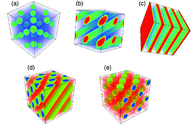
Figure 1: Nuclear pasta phases in a relativistic mean-field model of low density nuclear matter. The panels show a progression from “meatball” (a) to “spaghetti” (b) to “lasagna” (c) to “macaroni” (d) to “swiss cheese” (e) phases, which are the numerically obtained candidates for the ground state at different nuclear densities. Reproduced from Ref. [25].

Within the liquid drop model, the simplest way to introduce confinement is to restrict the nuclear fluid to a bounded domain and impose a particular choice of boundary conditions for the Coulombic potential. Then, after a suitable non-dimensionalization the energy takes the form

$$E(u):=\int_{\Omega}|\nabla u|\,dx+\frac{1}{2}\int_{\Omega}\int_{\Omega}G(x,y)(u(x)-\bar{u})(u(y)-\bar{u})\,dx\,dy.$$ (1.1)

Here, $\Omega\subset\mathbb{R}^{3}$ is the spatial domain (bounded), $u\in BV(\Omega;\{0,1\})$ is the characteristic function of the region occupied by the nuclear fluid (nuclear fluid density), $\bar{u}\in(0,1)$ is the neutralizing uniform background density of electrons, and $G$ is the Green’s function of the Laplacian which, in the case of Neumann boundary conditions for the electrostatic potential solves

$$-\Delta_{x}G(x,y)=\delta(x-y)-{1\over|\Omega|},$$ (1.2)

where $\delta(x)$ is the Dirac delta-function. The nuclear fluid density must also satisfy the global electroneutrality constraint:

$${1\over|\Omega|}\int_{\Omega}u\,dx=\bar{u}.$$ (1.3)

In writing (1.1) we took into account that because of the scaling properties of the Green’s function one can eliminate all the physical constants appearing in (1.1) by choosing the appropriate energy and length scales.

It is notable that the model in (1.1)–(1.3) also appears in a completely different physical context, namely, in the studies of mesoscopic phases of diblock copolymer melts, where it is referred to as the Ohta-Kawasaki model [27, 28, 29]. This is, of course, not surprising, considering the fundamental nature of Coulomb forces. In fact, the range of applications of the energy in (1.1) goes far beyond the systems mentioned above (for an overview, see [30] and references therein). Importantly, the model in (1.1) is a paradigm for the energy-driven pattern forming systems in which spatial patterns (global or local energy minimizers) form as a result of the competition of short-range attractive and long-range repulsive forces. This is why this model and its generalizations attracted considerable attention of mathematicians in recent years (see, e.g., [31, 32, 33, 34, 35, 36, 37, 38, 39, 40, 41, 42, 43, 44, 45, 46, 47, 48, 49], this list is certainly not exhaustive). In particular, the volume-constrained global minimization problem for (1.1) in the whole space with no neutralizing background, which we will also refer to as the “self-energy problem”, has been investigated in [34, 37, 45, 49].

A question of particular physical interest is how the ground states of the energy in (1.1) behave as the domain size tends to infinity. In [32], Alberti, Choksi and Otto showed that in this so-called “macroscopic” limit the energy becomes distributed uniformly throughout the domain. Another asymptotic regime, corresponding to the onset of non-trivial minimizers in the two-dimensional screened version of (1.1) was studied in [33], where it was shown that at appropriately low densities every non-trivial minimizer is given by the characteristic function of a collection of nearly perfect, identical, well separated small disks (droplets) uniformly distributed throughout the domain (see also [38] for a related study of almost minimizers). Further results about the fine properties of the minimizers were obtained via two-scale $\Gamma$-expansion in [39], using the approach developed for the studies of magnetic Ginzburg-Landau vortices [50] (more recently, the latter was also applied to three-dimensional Coulomb gases [51]). In particular, the method of [39] allows, in principle, to determine the asymptotic spatial arrangement of the droplets of the low density phase via the solution of a minimization problem involving point charges in the plane. It is widely believed that the solution of this problem should be given by a hexagonal lattice, which in the context of type-II superconductors is called the “Abrikosov lattice” [52]. Proving this result rigorously is a formidable task, and to date such a result has been obtained only within a much reduced class of Bravais lattices [53, 50].

It is natural to ask what happens with the low density ground state of the energy in (1.1) as the size of the domain $\Omega$ goes to infinity in three space dimensions. As can be seen from the above discussion, the answer to this question bears immediate relevance to the structure of nuclear matter under the conditions realized in the outer crust of neutron stars. This is the question that we address in the present paper. On physical grounds, it is expected that at low densities the ground state of such systems is given by the characteristic function of a union of nearly perfect small balls (nuclei) arranged into a body-centered cubic lattice (known to minimize the Coulomb energy of point charges among body-centered cubic, face-centered cubic and hexagonal close-packed lattices [54, 55, 56]). The volume of each nucleus should maximize the binding energy per nucleon, which then yields the nucleus of an isotope of nickel.

Our results concerning the minimizers of (1.1) proceed in that direction, but are still far from rigorously establishing such a detailed physical picture. One major difficulty has to do with the lack of the complete solution of the self-energy problem [37, 48]. Assuming the solution of this problem, whenever it exists, is a spherical droplet, a mathematical conjecture formulated by Choksi and Peletier [35] and a universally accepted hypothesis in nuclear physics, we indeed recover spherical nuclei whose volume minimizes the self-energy per unit nuclear volume (which is equivalent to maximizing the binding energy per nucleon in the nuclear context). The question of spatial arrangement of the nuclei is another major difficulty related to establishing periodicity of ground states of systems of interacting particles, which goes far beyond the scope of the present paper. Nevertheless, knowing that the optimal droplets are spherical should make it possible to apply the techniques of [50, 51] to relate the spatial arrangement of droplets to that of the minimizers of the renormalized Coulomb energy.

In the absence of the complete solution of the self-energy problem, we can still establish, although in a somewhat implicit manner, the limit behavior of the minimizers of (1.1)–(1.3) in the case $\Omega={\mathbb{T}}_{\ell}$, where ${\mathbb{T}}_{\ell}$ is the three-dimensional torus with sidelength $\ell$, as $\ell\to\infty$, provided that $\bar{u}$ also goes simultaneously to zero with an appropriate rate (low-density regime). We do so by establishing the $\Gamma$-limit of the energy in (1.1), with the notion of convergence given by weak convergence of measures (for a closely related study, see [38]). The limit energy is given by the sum of a constant term proportional to the volume occupied by the minority phase (which is also referred to as “mass” throughout the paper) and the Coulombic energy of the limit measure, with the proportionality constant in the first term given by the minimal self-energy per unit mass among all masses for which the minimum of the self-energy is attained. Importantly, the minimizer of the limit energy (which is strictly convex) is given uniquely by the uniform measure. Thus, we establish that for a minimizer of (1.1)–(1.3) the mass in the minority phase spreads (in a coarse-grained sense) uniformly throughout the spatial domain and that the minimal energy is proportional to the mass, with the proportionality constant given by the minimal self-energy per unit mass (compare to [32]). We also establish that almost all the “droplets”, i.e., the connected components of the support of a particular minimizer, are close to the minimizers of the self-energy with mass that minimizes the self-energy per unit mass.

Mathematically, it would be natural to try to extend our results in two directions. The first direction is to consider exactly the same energy as in (1.1) in higher space dimensions. Here, however, we encounter a difficulty that it is not known that the minimizers of the self-energy do not exist for large enough masses. Such a result is only available in three space dimensions for the Coulombic kernel [37, 45]. In the absence of such a non-existence result one may not exclude a possibility of a network-like structure in the macroscopic limit. Another direction is to replace the Coulombic kernel in (1.1) with the one corresponding to a more general negative Sobolev norm. Here we would expect our results to still hold in two space dimensions. Furthermore, the physical picture of identical radial droplets in the limit is expected for sufficiently long-ranged kernels, i.e., those kernels that satisfy $G(x,y)\sim|x-y|^{-\alpha}$ for $|x-y|\ll 1$, with $0<\alpha\ll 1$ [36, 47]. Note that although a similar characterization of the minimizers for long-ranged kernels exists in higher dimensions as well [44, 46], these results are still not sufficient to be used to characterize the limit droplets, since they do not give an explicit interval of existence of the minimizers of the self-interaction problem. Also, since the non-existence result for the self-energy with such kernels is available only for $\alpha<2$ [37], our results may not extend to the case of $\alpha\geq 2$ in dimensions three and above.

Finally, a question of both physical and mathematical interest is what happens with the above picture when the Coulomb potential is screened (e.g., by the background density fluctuations). In the simplest case, one would replace (1.2) with the following equation defining $G$:

$$-\Delta_{x}G(x,y)+\kappa^{2}G(x,y)=\delta(x-y),$$ (1.4)

where $\kappa>0$ is the inverse screening length, and the charge neutrality constraint from (1.3) is relaxed. Here a bifurcation from trivial to non-trivial ground states is expected under suitable conditions (in two dimensions, see [33, 38, 39]). We speculate that in certain limits this case may give rise to non-spherical droplets that minimize the self-energy. Indeed, in the presence of an exponential cutoff at large distances, it may no longer be advantageous to split large droplets into smaller disconnected pieces, and the self-energy minimizers for arbitrarily large masses may exist and resemble a “kebab on a skewer”. In contrast to the bare Coulomb case, in the screened case the energy of such a kebab-shaped configuration scales linearly with mass. Note that this configuration is reminiscent of the pearl-necklace morphology exhibited by long polyelectrolyte molecules in poor solvents [57, 58].

Organization of the paper.

In Sec. 2, we introduce the specific model, the scaling regime considered, the functional setting and the heuristics. In this section, we also discuss the self-energy problem and mention a result about attainment of the optimal self-energy per unit mass. In Sec. 3, we first state a basic existence and regularity result for the minimizers (Theorem 3.1) and give a characterization of the minimizers of the whole space problem that also minimize the self-energy per unit mass (Theorem 3.2). We then state our main $\Gamma$-convergence result in Theorem 3.3. In the same section, we also state the consequences of Theorem 3.3 to the asymptotic behavior of the minimizers in Corollary 3.4, as well as Theorem 3.5 about the uniform distribution of energy in the minimizers and Theorem 3.6 that establishes the multidroplet character of the minimizers. Section 4 is devoted to generalized minimizers of the self-energy problem, where, in particular, we obtain existence and uniform regularity for minimizers in Theorem 4.5 and Theorem 4.7. This section also establishes a connection to the minimizers of the whole space problem with a truncated Coulombic kernel and ends with a characterization of the optimal self-energy per unit mass in Theorem 4.15. Section 5 contains the proof of the $\Gamma$-convergence result of Theorem 3.3 and of the equidistribution result of Theorem 3.5. Section 6 establishes uniform estimates for the problem on the rescaled torus, where, in particular, uniform estimates for the potential are obtained in Theorem 6.9. Section 7 presents the proof of Theorem 3.6. Finally, some technical results concerning the limit measures appearing in the $\Gamma$-limit are collected in the Appendix.

Notation.

Throughout the paper $H^{1}$, $BV$, $L^{p}$, $C^{k}$, $C^{k}_{c}$, $C^{k,\alpha}$, $\mathcal{M}$ denote the usual spaces of Sobolev functions, functions of bounded variation, Lebesgue functions, functions with continuous derivatives up to order $k$, compactly supported functions with continuous derivatives up to order $k$, functions with Hölder-continuous derivatives up to order $k$ for $\alpha\in(0,1)$, and the space of finite signed Radon measures, respectively. We will use the symbol $|\nabla u|$ to denote the Radon measure associated with the distributional gradient of a function of bounded variation. With a slight abuse of notation, we will also identify Radon measures with the associated, possibly singular, densities (with respect to the Lebesgue measure) on the underlying spatial domain. For example, we will write $\nu=|\nabla u|$ and $d\nu(x)=|\nabla u(x)|\,dx$ to imply $\nu\in\mathcal{M}(\Omega)$ and $\nu(\Omega^{\prime})=|\nabla u|(\Omega^{\prime})=\int_{\Omega^{\prime}}|\nabla u|\,dx$, given $u\in BV(\Omega)$ and $\Omega^{\prime}\subset\Omega$. For a set $I\subset\mathbb{N}$, $\#I$ denotes cardinality of $I$. The symbol $\chi_{F}$ always stands for the characteristic function of the set $F$, and $|F|$ denotes its Lebesgue measure. We also use the notation $(u_{\varepsilon})\in\mathcal{A}_{\varepsilon}$ to denote sequences of functions $u_{\varepsilon}\in\mathcal{A}_{\varepsilon}$ as $\varepsilon=\varepsilon_{n}\to 0$, where $\mathcal{A}_{\varepsilon}$ are admissible classes.

2 Mathematical setting and scaling

Variational problem on the unit torus.

Throughout the rest of this paper the spatial domain $\Omega$ in (1.1) is assumed to be a torus, which allows us to avoid dealing with boundary effects and concentrate on the bulk properties of the energy minimizers. We define ${\mathbb{T}}:=\mathbb{R}^{3}/\mathbb{Z}^{3}$ to be the flat three-dimensional torus with unit sidelength. For $\varepsilon>0$, which should be treated as a small parameter, we introduce the following energy functional:

$$E_{\varepsilon}(u)\ :=\ \varepsilon\int_{\mathbb{T}}|\nabla u|\,dx+\frac{1}{2}\int_{\mathbb{T}}(u-\bar{u}_{\varepsilon})(-\Delta)^{-1}(u-\bar{u}_{\varepsilon})\,dx,$$ (2.1)

where the first term is understood distributionally and the second term is understood as the double integral involving the periodic Green’s function of the Laplacian, with $u$ belonging to the admissible class

$${\mathcal{A}}_{\varepsilon}\ :=\ \left\{u\in BV({\mathbb{T}};\{0,1\})\ :\ \int_{\mathbb{T}}u\,dx=\bar{u}_{\varepsilon}\right\},$$ (2.2)

where

$$\bar{u}_{\varepsilon}:=\lambda\,\varepsilon^{2/3},$$ (2.3)

with some fixed $\lambda>0$. The choice of the scaling of $\bar{u}_{\varepsilon}$ with $\varepsilon$ in (2.3) will be explained shortly. To simplify the notation, we suppress the explicit dependence of the admissible class on $\lambda$, which is fixed throughout the paper.

It is natural to define for $u\in{\mathcal{A}}_{\varepsilon}$ the measure $\mu_{\varepsilon}$ by

$$d\mu_{\varepsilon}(x):=\varepsilon^{-{2/3}}u(x)\,dx.$$ (2.4)

In particular, $\mu_{\varepsilon}$ is a positive Radon measure and satisfies $\mu_{\varepsilon}({\mathbb{T}})=\lambda$. Therefore, on a suitable sequence as $\varepsilon\to 0$ the measure $\mu_{\varepsilon}$ converges weakly in the sense of measures to a limit measure $\mu$, which is again a positive Radon measure and satisfies $\mu({\mathbb{T}})=\lambda$.

Function spaces for the measure and potential.

In terms of $\mu_{\varepsilon}$ the Coulombic term in (2.1) is given by

$$\frac{1}{2}\int_{\mathbb{T}}(u-\bar{u}_{\varepsilon})(-\Delta)^{-1}(u-\bar{u}_{\varepsilon})\,dx=\frac{\varepsilon^{4/3}}{2}\int_{\mathbb{T}}\int_{\mathbb{T}}G(x-y)\,d\mu_{\varepsilon}(x)\,d\mu_{\varepsilon}(y),$$ (2.5)

where $G$ is the periodic Green’s function of the Laplacian on ${\mathbb{T}}$, i.e., the unique distributional solution of

$$-\Delta G(x)=\delta(x)-1,\qquad\qquad\int_{{\mathbb{T}}}G(x)\,dx=0.$$ (2.6)

If the kernel $G$ in (2.5) were smooth, then one would be able to pass directly to the limit in the Coulombic term and obtain the corresponding convolution of the kernel with the limit measure. This is not possible due to the singularity of the kernel at $\{x=y\}$. In fact, the double integral involving the limit measure may be strictly less than the $\liminf$ of the sequence, and the defect of the limit is related to a non-trivial contribution of the self-interaction of the connected components of the set $\{u=1\}$ and its perimeter to the limit energy.

On the other hand, the singular character of the kernel provides control on the regularity of the limit measure $\mu$. To see this, we define the electrostatic potential $v_{\varepsilon}\in H^{1}({\mathbb{T}})$ by

$$v_{\varepsilon}(x):=\int_{\mathbb{T}}G(x-y)\,d\mu_{\varepsilon}(y),$$ (2.7)

which solves

$$\int_{\mathbb{T}}\nabla\varphi\cdot\nabla v_{\varepsilon}\,dx=\int_{\mathbb{T}}\varphi\,d\mu_{\varepsilon}-\lambda\int_{\mathbb{T}}\varphi\,dx\qquad\qquad\forall\varphi\in C^{\infty}({\mathbb{T}}).$$ (2.8)

By (2.4), we can rewrite the corresponding term in the Coulombic energy as

$$\int_{\mathbb{T}}\int_{\mathbb{T}}G(x-y)\,d\mu_{\varepsilon}(x)\,d\mu_{\varepsilon}(y)=\int_{\mathbb{T}}v_{\varepsilon}\,d\mu_{\varepsilon}=\int_{\mathbb{T}}|\nabla v_{\varepsilon}|^{2}\,dx.$$ (2.9)

Hence, if the left-hand side of (2.9) remains bounded as $\varepsilon\to 0$, and since $\int_{\mathbb{T}}v_{\varepsilon}\,dx=0$, the sequence $v_{\varepsilon}$ is uniformly bounded in $H^{1}({\mathbb{T}})$ and hence weakly convergent in $H^{1}({\mathbb{T}})$ on a subsequence.

By the above discussion, the natural space for the potential is the space

$$\mathcal{H}\ :=\ \left\{v\in H^{1}({\mathbb{T}}):\int_{\mathbb{T}}v\,dx=0\right\} \|v\|_{\mathcal{H}}\ :=\ \left(\int_{\mathbb{T}}|\nabla v|^{2}\,dx\right)^{1/2}.$$ with (2.10)

The space $\mathcal{H}$ is a Hilbert space together with the inner product

$$\langle u,v\rangle_{\mathcal{H}}:=\int_{\mathbb{T}}\nabla u\cdot\nabla v\,dx\qquad\qquad\forall u,v\in\mathcal{H}.$$ (2.11)

The natural class for measures $\mu_{\varepsilon}$ to consider is the class of positive Radon measures on ${\mathbb{T}}$ which are also in $\mathcal{H}^{\prime}$, the dual of $\mathcal{H}$. More precisely, let ${\mathcal{M}}^{+}({\mathbb{T}})\subset{\mathcal{M}}({\mathbb{T}})$ be the set of all positive Radon measures on ${\mathbb{T}}$. We define the subset ${\mathcal{M}}^{+}({\mathbb{T}})\cap\mathcal{H}^{\prime}$ of ${\mathcal{M}}^{+}({\mathbb{T}})$ by

$${\mathcal{M}}^{+}({\mathbb{T}})\cap\mathcal{H}^{\prime}=\Big{\{}\mu\in{\mathcal{M}}^{+}({\mathbb{T}})\ :\ \int_{\mathbb{T}}\varphi\,d\mu\leq C\|\varphi\|_{\mathcal{H}}\ \ \ \forall\varphi\in\mathcal{H}\cap C({\mathbb{T}})\Big{\}},$$ (2.12)

for some $C>0$. This is the set of positive Radon measures which can be understood as continuous linear functionals on $\mathcal{H}$. Note that $\mu\in{\mathcal{M}}^{+}({\mathbb{T}})$ satisfies $\mu\in{\mathcal{M}}^{+}({\mathbb{T}})\cap\mathcal{H}^{\prime}$ if and only if it has finite Coulombic energy, i.e.

$$\int_{\mathbb{T}}\int_{\mathbb{T}}G(x-y)\,d\mu(x)\,d\mu(y)<\infty,$$ (2.13)

with the convention that $G(0)=+\infty$. The proof of this characterization and related facts about ${\mathcal{M}}^{+}({\mathbb{T}})\cap\mathcal{H}^{\prime}$ are given in the Appendix.

The whole space problem.

We will also consider the following related problem, formulated on ${\mathbb{R}}^{3}$. We consider the energy

$$\widetilde{E}_{\infty}(u)\ :=\ \int_{\mathbb{R}^{3}}|\nabla u|\,dx+{1\over 8\pi}\int_{\mathbb{R}^{3}}\int_{\mathbb{R}^{3}}{u(x)u(y)\over|x-y|}\,dx\,dy.$$ (2.14)

The appropriate admissible class for the energy $\widetilde{E}_{\infty}$ in the present context is that of configurations with prescribed “mass” $m>0$:

$$\widetilde{\mathcal{A}}_{\infty}(m):=\left\{u\in BV({\mathbb{R}}^{3};\{0,1\})\ :\int_{\mathbb{R}^{3}}u\,dx=m\right\}.$$ (2.15)

For a given mass $m>0$, we define the minimal energy by

$$e(m)\ :=\ \inf_{u\in\widetilde{A}_{\infty}(m)}\widetilde{E}_{\infty}(u).$$ (2.16)

The set of masses for which the infimum of $\widetilde{E}_{\infty}$ in $\widetilde{A}_{\infty}(m)$ is attained is denoted by

$$\mathcal{I}:=\left\{m\geq 0\ :\ \exists\ u_{m}\in\widetilde{A}_{\infty}(m),\ \widetilde{E}_{\infty}(u_{m})=e(m)\right\},$$ (2.17)

The minimization problem associated with (2.14) and (2.15) was recently studied by two of the authors in [37]. In particular, by [37, Theorem 3.3] the set $\mathcal{I}$ is bounded, and by [37, Theorems 3.1 and 3.2] the set ${\mathcal{I}}$ is non-empty and contains an interval around the origin.

For $m\geq 0$, we also define the quantity (with the convention that $f(0):=+\infty$)

$$f(m):={e(m)\over m},$$ (2.18)

which represents the minimal energy for (2.14) and (2.15) per unit mass. By [37, Theorem 3.2] there is a universal $\widetilde{m}_{0}>0$ such that $f(m)$ is obtained by evaluating $\widetilde{E}_{\infty}$ on a ball of mass $m$ for all $m\leq\widetilde{m}_{0}$. After a simple computation, this yields

$$f(m)=6^{2/3}\pi^{1/3}m^{-1/3}+3^{2/3}\cdot 2^{-1/3}\cdot 10^{-1}\cdot\pi^{-2/3}m^{2/3}\qquad\text{for all }0<m\leq\widetilde{m}_{0}.$$ (2.19)

Note that obviously this expression also gives an a priori upper bound for $f(m)$ for all $m>0$. In addition, by [37, Theorem 3.4] there exist universal constants $C,c>0$ such that

$$c\leq f(m)\leq C\qquad\text{for all}\ m\geq\widetilde{m}_{0}.$$ (2.20)

It was conjectured in [35] that $\mathcal{I}=[0,\widetilde{m}_{0}]$ and that $\widetilde{m}_{0}=m_{c1}$, where

$$m_{c1}:=\frac{40\pi}{3}\left(2^{1/3}+2^{-1/3}-1\right)\approx 44.134.$$ (2.21)

The quantity $m_{c1}$ is the maximum value of $m$ for which a ball of mass $m$ has less energy than twice the energy of a ball with mass $\frac{1}{2}m$. However, such a result is not available at present and remains an important challenge for the considered class of variational problems (for several related results see [36, 44, 47]).

Finally, we define

$$f^{*}:=\inf_{m\in\mathcal{I}}f(m) \mathcal{I}^{*}:=\left\{m^{*}\in\mathcal{I}\ :\ f(m^{*})=f^{*}\right\}.$$ and (2.22)

Observe that in view of (2.19) and (2.20) we have $f^{*}\in(0,\infty)$. Also, as we will show in Theorem 3.2, the set $\mathcal{I}^{*}$ is non-empty, i.e., the minimum of $f(m)$ over $\mathcal{I}$ is attained. In fact, the minimum of $f(m)$ over $\mathcal{I}$ is also the minimum over all $m\in(0,\infty)$ (see Theorem 4.15). Note that this result was also independently obtained by Frank and Lieb in their recent work [49]. The set $\mathcal{I}^{*}$ of masses that minimize the energy $\widetilde{E}_{\infty}$ per unit mass and the associated minimizers (which in general may not be unique) will play a key role in the analysis of the limit behavior of the minimizers of $E_{\varepsilon}$. Note that if $f(m)$ were given by (2.19) and $\mathcal{I}=[0,m_{c1}]$, then we would have explicitly $\mathcal{I}^{*}=\{10\pi\}$ and $f^{*}=3^{5/3}\cdot 2^{-2/3}\cdot 5^{-1/3}\approx 2.29893$. On the other hand, in view of the statement following (2.19), this value provides an a priori upper bound on the optimal energy density.

Macroscopic limit & heuristics.

The limit $\varepsilon\to 0$ with $\lambda>0$ fixed is equivalent to the limit of the energy in (1.1) with $\Omega={\mathbb{T}}_{\ell}$, where ${\mathbb{T}}_{\ell}:=\mathbb{R}^{3}/(\ell\mathbb{Z})^{3}$ is the torus with sidelength $\ell>0$, as $\ell\to\infty$. Indeed, introducing the notation

$$\widetilde{E}_{\ell}(\tilde{u})\ :=\ \int_{{\mathbb{T}_{\ell}}}|\nabla\tilde{u}|\,dx+\frac{1}{2}\int_{\mathbb{T}_{\ell}}(\tilde{u}-\bar{\tilde{u}}_{\ell})(-\Delta)^{-1}(\tilde{u}-\bar{\tilde{u}}_{\ell})\,dx,$$ (2.23)

for the energy in (1.1) with $\Omega={\mathbb{T}}_{\ell}$, and taking $\bar{\tilde{u}}_{\ell}=\lambda\ell^{-2}$ and $\tilde{u}\in\widetilde{\mathcal{A}}_{\ell}$, where

$$\widetilde{\mathcal{A}}_{\ell}\ :=\ \left\{\tilde{u}\in BV({\mathbb{T}_{\ell}};\{0,1\})\ :\ \int_{\mathbb{T}_{\ell}}\tilde{u}\,dx=\lambda\ell\right\},$$ (2.24)

it is easy to see that $u(x):=\tilde{u}(\ell x)$ belongs to $\mathcal{A}_{\varepsilon}$ with $\bar{u}_{\varepsilon}=\lambda\varepsilon^{2/3}$ for $\varepsilon=\ell^{-3}$, and we have $E_{\varepsilon}(u)=\ell^{-5}\widetilde{E}_{\ell}(\tilde{u})$. It then follows that the two limits $\ell\to\infty$ and $\varepsilon\to 0$ are equivalent. Note that the full space energy $\widetilde{E}_{\infty}$ is the formal limit of (2.23) for $\ell\to\infty$.

The choice of the scaling of $\bar{u}_{\varepsilon}$ with $\varepsilon$ is determined by the balance of far-field and near-field contributions of the Coulomb energy. Heuristically, one would expect the minimizers of the energy in (2.1) to be given by the characteristic function of a set that consists of “droplets” of size of order $R\ll 1$ separated by distance of order $d$ satisfying $R\ll d\ll 1$ (for evidence based on recent molecular dynamics simulations, see also [26]). Assuming that the volume of each droplet scales as $R^{3}$ (think, for example, of all the droplets as non-overlapping balls of equal radius and with centers forming a periodic lattice), from (2.23) we find for the surface energy, self-energy and interaction energy, respectively, for a single droplet:

$$E_{\mathrm{surf}}\sim\varepsilon R^{2},\qquad E_{\mathrm{self}}\sim R^{5},\qquad E_{\mathrm{int}}\sim{R^{6}\over d^{3}}.$$ (2.25)

Equating these three quantities and recalling that $R^{3}/d^{3}\sim\bar{u}_{\varepsilon}$, we obtain

$$R\sim\varepsilon^{1/3},\qquad d\sim\varepsilon^{1/9},\qquad\bar{u}_{\varepsilon}\sim\varepsilon^{2/3},$$ (2.26)

which leads to (2.3). Note that, in some sense, this is the most interesting low volume fraction regime that leads to infinitely many droplets in the limit as $\varepsilon\to 0$, since both the self-energy of each droplet and the interaction energy between different droplets contribute comparably to the energy. For other scalings one would expect only one of these two terms to contribute in the limit, which would, however, result in loss of control on either the perimeter term or the Coulomb term as $\varepsilon\to 0$ and, as a consequence, a possible change in behavior. Let us note that a different scaling regime, in which $\bar{u}_{\varepsilon}=O(\varepsilon)$, leads instead to finitely many droplets that concentrate on points as $\varepsilon\to 0$ [34], while for $\bar{u}_{\varepsilon}=O(1)$ one expects phases of reduced dimensionality, such as rods and slabs (see Fig. 1).

3 Statement of the main results

We now turn to stating the main results of this paper concerning the asymptotic behavior of the minimizers or the low energy configuration of the energy in (2.1) within the admissible class in (2.2). Existence of these minimizers is guaranteed by the following theorem.

Theorem 3.1 (Minimizers: existence and regularity).

For every $\lambda>0$ and every $0<\varepsilon<\lambda^{-3/2}$ there exists a minimizer $u_{\varepsilon}\in\mathcal{A}_{\varepsilon}$ of $E_{\varepsilon}$ given by (2.1) with $\bar{u}_{\varepsilon}$ given by (2.3). Furthermore, after a possible modification of $u_{\varepsilon}$ on a set of zero Lebesgue measure the support of $u_{\varepsilon}$ has boundary of class $C^{\infty}$.

Proof.

The proof of Theorem 3.1 is fairly standard. We present a few details below for the sake of completeness.

By the direct method of the calculus of variations, minimizers of the considered problem exist for all $\varepsilon>0$ as soon as the admissible class $\mathcal{A}_{\varepsilon}$ is non-empty, in view of the fact that the first term is coercive and lower semicontinuous in $BV({\mathbb{T}})$, and that the second term is continuous with respect to the $L^{1}({\mathbb{T}})$ convergence of characteristic functions. The admissible class is non-empty if and only if $\varepsilon<\lambda^{-3/2}$.

Hölder regularity of minimizers was proved in [59, Proposition 2.1], where it was shown that the essential support of minimizers has boundary of class $C^{3,\alpha}$. Smoothness of the boundary was established in [43, Proposition 2.2] (see also the proof of Lemma 4.4 below for a brief outline of the argument in a closely related context). ∎

In view of the regularity statement above, throughout the rest of the paper we always choose the regular representative of a minimizer.

We proceed by giving a characterization of the quantity $f^{*}$ defined in (2.22) as the minimal self-energy of a single droplet per unit mass, i.e., as the minimum of $f(m)$ over $\mathcal{I}$.

Theorem 3.2 (Self-energy: attainment of optimal energy per unit mass).

Let $f^{*}$ be defined as in (2.22). Then there exists $m^{*}\in\mathcal{I}$ such that $f^{*}=f(m^{*})$.

With the result in Theorem 3.2, we are now in the position to state our main result on the $\Gamma$-limit of the energy in (2.1), which can be viewed as a generalization of [38, Theorem 1].

Theorem 3.3 ($\Gamma$-convergence).

For a given $\lambda>0$, let $E_{\varepsilon}$ be defined by (2.1) with $\bar{u}_{\varepsilon}$ given by (2.3). Then as $\varepsilon\to 0$ we have $\varepsilon^{-{4/3}}E_{\varepsilon}\stackrel{{\scriptstyle\Gamma}}{{\to}}E_{0}$, where

$$E_{0}(\mu):=\lambda f^{*}+\frac{1}{2}\int_{\mathbb{T}}\int_{\mathbb{T}}G(x-y)\,d\mu(x)\,d\mu(y),$$ (3.1)

and $\mu\in{\mathcal{M}}^{+}({\mathbb{T}})\cap\mathcal{H}^{\prime}$ satisfies $\mu({\mathbb{T}})=\lambda$. More precisely,

• (Compactness and $\Gamma$-liminf inequality) Let $(u_{\varepsilon})\in\mathcal{A}_{\varepsilon}$ be such that

  $$\limsup_{\varepsilon\to 0}\varepsilon^{-4/3}E_{\varepsilon}(u_{\varepsilon})<\infty,$$ (3.2)

  and let $\mu_{\varepsilon}$ and $v_{\varepsilon}$ be defined in (2.4) and (2.7), respectively. Then, upon extraction of a subsequence, we have

  $$\mu_{\varepsilon}\rightharpoonup\mu\textrm{ in }{\mathcal{M}}({\mathbb{T}}),\qquad v_{\varepsilon}\rightharpoonup v\textrm{ in }\mathcal{H},$$ (3.3)

  as $\varepsilon\to 0$, for some $\mu\in{\mathcal{M}}^{+}({\mathbb{T}})\cap\mathcal{H}^{\prime}$ with $\mu({\mathbb{T}})=\lambda$, the function $v$ has a representative in $L^{1}({\mathbb{T}},d\mu)$ given by

  $$v(x)=\int_{\mathbb{T}}G(x-y)\,d\mu(y),$$ (3.4)

  and

  $$\liminf_{\varepsilon\to 0}\varepsilon^{-4/3}E_{\varepsilon}(u_{\varepsilon})\geq E_{0}(\mu).$$ (3.5)

• ($\Gamma$-limsup inequality) For any measure $\mu\in{\mathcal{M}}^{+}({\mathbb{T}})\cap\mathcal{H}^{\prime}$ with $\mu({\mathbb{T}})=\lambda$ there exists a sequence $(u_{\varepsilon})\in\mathcal{A}_{\varepsilon}$ such that (3.3) and (3.4) hold as $\varepsilon\to 0$ for $\mu_{\varepsilon}$ and $v_{\varepsilon}$ defined in (2.4) and (2.7), and

  $$\limsup_{\varepsilon\to 0}\varepsilon^{-4/3}E_{\varepsilon}(u_{\varepsilon})\leq E_{0}(\mu).$$ (3.6)

Note that the weak convergence of measures was recently identified in [38] (see also [33]) as a suitable notion of convergence for the studies of the $\Gamma$-limit of the two-dimensional version of the energy in (2.1).

Observe also that the limit energy $E_{0}$ is a strictly convex functional of the limit measure and, hence, attains a unique global minimum. By direct inspection, $E_{0}$ is minimized by $\mu=\mu_{0}$, where $d\mu_{0}:=\lambda dx$. Thus, the quantity $f^{*}$ plays the role of the optimal energy density in the limit $\varepsilon\to 0$.

The remaining results are concerned with sequences of minimizers. We will hence assume that the functions $(u_{\varepsilon})\in{\mathcal{A}}_{\varepsilon}$ are minimizers of the functional $E_{\varepsilon}$. In this case, we can give a more precise characterization for the asymptotic behavior of the sequence. We first note the following immediate consequence of Theorem 3.3 for the convergence of sequences of minimizers.

Corollary 3.4 (Minimizers: uniform distribution of mass).

For $\lambda>0$, let $(u_{\varepsilon})\in\mathcal{A}_{\varepsilon}$ be minimizers of $E_{\varepsilon}$, and let $\mu_{\varepsilon}$ and $v_{\varepsilon}$ be defined in (2.4) and (2.7), respectively. Then

$$\mu_{\varepsilon}\rightharpoonup\mu_{0}\textrm{ in }\mathcal{M}({\mathbb{T}}),\qquad v_{\varepsilon}\rightharpoonup 0\textrm{ in }\mathcal{H},$$ (3.7)

where $d\mu_{0}=\lambda dx$, and

$$\varepsilon^{-4/3}E_{\varepsilon}(u_{\varepsilon})\to\lambda f^{*},$$ (3.8)

where $f^{*}$ is as in (2.22), as $\varepsilon\to 0$.

The formula in (3.8) suggests that in the limit the energy of the minimizers is dominated by the self-energy, which is captured by the minimization problem associated with the energy $\widetilde{E}_{\infty}$ defined in (2.14). Therefore, it would be natural to expect that asymptotically every connected component of a minimizer is close to a minimizer of $\widetilde{E}_{\infty}$ under the mass constraint associated with that connected component. Note that in a closely related problem in two space dimensions such a result was established in [33] for minimizers, and in [38, 39] for almost minimizers. The situation is, however, unique in two space dimensions, because the non-local term in some sense decouples from the perimeter term. Hence, the minimizers behave as almost minimizers of the perimeter and, therefore, are close to balls. In three dimensions, however, the perimeter and the non-local term of the self-energy $\widetilde{E}_{\infty}$ are fully coupled, and, therefore, rigidity estimates for the perimeter functional alone [60] may not be sufficient to conclude about the “shape” of the minimizers. Nevertheless, we are able to prove a result about the uniform distribution of the energy density of the minimizers as $\varepsilon\to 0$ in the spirit of that of [32]. For a minimizer $u_{\varepsilon}$, the energy density is associated with the Radon measure $\nu_{\varepsilon}$ defined by

$$d\nu_{\varepsilon}:=\varepsilon^{-4/3}\Big{(}\varepsilon|\nabla u_{\varepsilon}|+\tfrac{1}{2}\varepsilon^{2/3}u_{\varepsilon}v_{\varepsilon}\Big{)}dx,$$ (3.9)

where $v_{\varepsilon}$ is given by (2.7) and (2.4). Furthermore, we are able to identify the leading order constant in the asymptotic behavior of the energy density.

Theorem 3.5 (Minimizers: uniform distribution of energy).

For $\lambda>0$, let $(u_{\varepsilon})\in\mathcal{A}_{\varepsilon}$ be minimizers of $E_{\varepsilon}$ and let $\nu_{\varepsilon}$ be defined in (3.9). Then

$$\nu_{\varepsilon}\rightharpoonup\nu_{0}\textrm{ in }{\mathcal{M}}({\mathbb{T}})\qquad\text{ as $\varepsilon\to 0$,}$$ (3.10)

where $d\nu_{0}=\lambda f^{*}dx$ and $f^{*}$ is as in (2.22).

Finally, we characterize the connected components of the support of the minimizers of $E_{\varepsilon}$ and show that almost all of them approach, on a suitable sequence as $\varepsilon\to 0$ and after a suitable rescaling and translation, a minimizer of $\widetilde{E}_{\infty}$ with mass in the set $\mathcal{I}^{*}$.

Theorem 3.6 (Minimizers: droplet structure).

For $\lambda>0$, let $(u_{\varepsilon})\in\mathcal{A}_{\varepsilon}$ be regular representatives of minimizers of $E_{\varepsilon}$, let $N_{\varepsilon}$ be the number of the connected components of the support of $u_{\varepsilon}$, let $u_{\varepsilon,k}\in BV({\mathbb{R}}^{3};\{0,1\})$ be the characteristic function of the $k$-th connected component of the support of the periodic extension of $u_{\varepsilon}$ to the whole of ${\mathbb{R}}^{3}$ modulo translations in $\mathbb{Z}^{3}$, and let $x_{\varepsilon,k}\in\mathrm{supp}(u_{\varepsilon,k})$. Then there exists $\varepsilon_{0}>0$ such that the following properties hold:

1. There exist universal constants $C,c>0$ such that for all $\varepsilon\leq\varepsilon_{0}$ we have

   $$\|v_{\varepsilon}\|_{L^{\infty}({\mathbb{T}})}\leq C\qquad\mathrm{and}\qquad\int_{{\mathbb{R}}^{3}}u_{\varepsilon,k}\,dx\geq c\varepsilon,$$ (3.11)

   where $v_{\varepsilon}$ is given by (2.7).

2. There exist universal constants $C,c>0$ such that for all $\varepsilon\leq\varepsilon_{0}$ we have

   $$\mathrm{supp}(u_{\varepsilon,k})\subseteq B_{C\varepsilon^{1/3}}(x_{\varepsilon,k})\qquad\mathrm{and}\qquad c\lambda\varepsilon^{-1/3}\leq N_{\varepsilon}\leq C\lambda\varepsilon^{-1/3}.$$ (3.12)

3. There exists $\widetilde{N}_{\varepsilon}\leq N_{\varepsilon}$ with $\widetilde{N}_{\varepsilon}/N_{\varepsilon}\to 1$ as $\varepsilon\to 0$ and a subsequence $\varepsilon_{n}\to 0$ such that for every $k_{n}\leq\widetilde{N}_{\varepsilon_{n}}$ the following holds: After possibly relabeling the connected components, we have

   $$\tilde{u}_{n}\to\tilde{u} \text{in $L^{1}({\mathbb{R}}^{3})$},$$ (3.13)

   where $\tilde{u}_{n}(x):=u_{\varepsilon_{n},k_{n}}(\varepsilon_{n}^{1/3}(x+x_{\varepsilon_{n},k_{n}}))$, and $\tilde{u}$ is a minimizer of $\widetilde{E}_{\infty}$ over $\widetilde{\mathcal{A}}_{\infty}(m^{*})$ for some $m^{*}\in\mathcal{I}^{*}$, where $\mathcal{I}^{*}$ is defined in (2.22).

The significance of this theorem lies in the fact that it shows that all the connected components of the support of a minimizer for sufficiently small $\varepsilon$ look like a collection of droplets of size of order $\varepsilon^{1/3}$ separated by distances of order $\varepsilon^{1/9}$ on average. In particular, the conclusion of the theorem excludes configurations that span the entire length of the torus, such as the “spaghetti” or “lasagna” phases of nuclear pasta (see Fig. 1). Thus, the ground state for small enough $\varepsilon>0$ is a multi-droplet pattern (a “meatball” phase). Furthermore, after a rescaling most of these droplets converge to minimizers of the non-local isoperimetric problem associated with $\widetilde{E}_{\infty}$ that minimize the self-energy per unit mass.

4 The problem in the whole space

In this section, we derive some results about the single droplet problem from (2.14)–(2.15) and the rescaled problem from (2.23)–(2.24).

4.1 The truncated energy $\widetilde{E}_{\infty}^{R}$

For reasons that will become apparent shortly, it is helpful to consider the energies where the range of the nonlocal interaction is truncated at certain length scale $R$. We choose a cut-off function $\eta\in C^{\infty}({\mathbb{R}})$ with $\eta^{\prime}(t)\leq 0$ for all $t\in{\mathbb{R}}$, $\eta(t)=1$ for all $t\leq 1$ and $\eta(t)=0$ for all $t\geq 2$. In the following, the choice of $\eta$ is fixed once and for all, and the dependence of constants on this choice is suppressed to avoid clutter in the presentation. For $R>0$, we then define $\eta_{R}\in C^{\infty}(\mathbb{R}^{3})$ by $\eta_{R}(x):=\eta(|x|/R)$. For $u\in\widetilde{\mathcal{A}}_{\infty}(m)$, we consider the truncated energy

$$\widetilde{E}_{\infty}^{R}(u):=\int_{{\mathbb{R}}^{3}}|\nabla u|\,dx+\int_{{\mathbb{R}}^{3}}\int_{{\mathbb{R}}^{3}}\frac{\eta_{R}(x-y)u(x)u(y)}{8\pi|x-y|}\,dx\,dy.$$ (4.1)

This functional will be useful in the analysis of the variational problems associated with $\widetilde{E}_{\infty}$ and $E_{\varepsilon}$. We recall that by the results of [61], for each $R>0$ and each $m>0$ there exists a minimizer of $\widetilde{E}_{\infty}^{R}$ in $\widetilde{\mathcal{A}}_{\infty}(m)$. Furthermore, after a possible redefinition on a set of Lebesgue measure zero, its support has boundary of class $C^{1,1/2}$ and consists of finitely many connected components. Below we always deal with the representatives of minimizers that are regular.

The following uniform density bound for minimizers of the energy is an adaption of [37, Lemma 4.3] for the truncated energy $\widetilde{E}_{\infty}^{R}$ and generalizes the corresponding bound for minimizers of $\widetilde{E}_{\infty}$.

Lemma 4.1 (Density bound).

There exists a universal constant $c>0$ such that for every minimizer $u\in\widetilde{\mathcal{A}}_{\infty}(m)$ of $\widetilde{E}_{\infty}^{R}$ for some $R,m>0$ and any $x_{0}\in\overline{F}$ we have

$$\int_{B_{r}(x_{0})}u\,dx\geq cr^{3}\qquad\text{for all }r\leq\min(1,m^{1/3}).$$ (4.2)

Proof.

The claim follows by an adaption of the proof of [37, Lemma 4.3] to our truncated energy $\widetilde{E}_{\infty}^{R}$. Indeed, it is enough to show that the statement of [37, Lemma 4.2] holds with $\widetilde{E}_{\infty}$ replaced by $\widetilde{E}_{\infty}^{R}$. The proof of this statement needs to be modified, since the kernel in the definition of $\widetilde{E}_{\infty}^{R}$ is not scale-invariant. We sketch the necessary changes, using the same notation as in [37].

The construction of the sets $\widetilde{F}$ and $\widehat{F}$ proceeds as in the proof of [37, Lemma 4.3]. The upper bound [37, Eq. (4.6)] still holds since $\widetilde{E}_{\infty}^{R}(u)\leq\widetilde{E}_{\infty}(u)$. Related to the cut-off function in the definition of $\widetilde{E}_{\infty}^{R}$, we get an additional term in the right-hand side of the first line of [37, Eq. (4.6)], which is of the form

$$\int_{\ell F_{1}}\int_{\ell F_{1}}{\eta_{R}(x-y)\over|x-y|^{\alpha}}\,dx\,dy-\ell^{2n-\alpha}\int_{F_{1}}\int_{F_{1}}{\eta_{R}(x-y)\over|x-y|^{\alpha}}\,dx\,dy\hskip 56.9055pt$$

$$=\ell^{2n-\alpha}\int_{F_{1}}\int_{F_{1}}{\eta_{R/\ell}(x-y)-\eta_{R}(x-y)\over|x-y|^{\alpha}}\,dx\,dy<0,$$ (4.3)

since $\ell>1$ and since the function $\eta$ is monotonically decreasing (note that $\alpha=1$ in our case). Since this term has a negative sign, [37, Eq. (4.6)] still holds. The rest of the argument then carries through unchanged. ∎

The following lemma establishes a uniform diameter bound for the minimizers of $\widetilde{E}_{\infty}^{R}$. The idea of the proof is similar to the one in [45, Lemma 5].

Lemma 4.2 (Diameter bound).

There exist universal constants $R_{0}>0$ and $D_{0}>0$ such that for any $R\geq R_{0}$, any $m>0$ and for any minimizer $u\in\widetilde{\mathcal{A}}_{\infty}(m)$ of $\widetilde{E}_{\infty}^{R}$, the diameter of each connected component $F_{0}$ of $\mathrm{supp}(u)$ is bounded above by $D_{0}$.

Proof.

Let $F_{0}$ be a connected component of the support of $u$ with $m_{0}:=|F_{0}|$. Since $u$ is a minimizer, $\chi_{F_{0}}$ is also a minimizer of $\widetilde{E}_{\infty}^{R}$ over $\mathcal{A}_{\infty}(m_{0})$. Indeed, if not, replacing $u$ with $u-\chi_{F_{0}}+\chi_{\widetilde{F}_{0}}$, where $\chi_{\widetilde{F}_{0}}$ is a minimizer of $\widetilde{E}_{\infty}^{R}$ over $\mathcal{A}_{\infty}(m_{0})$ translated sufficiently far from the support of $u$ would lower the energy, contradicting the minimizing property of $u$.

We may assume without loss of generality that $R\geq 2$ and ${\rm diam\ }F_{0}\geq 2$. Then there is $N\in{\mathbb{N}}$ such that $2N\leq{\rm diam\ }F_{0}<2(N+1)$. In particular there exist $x_{0},\ldots,x_{N}\in\overline{F}_{0}$ such that $|x_{k}-x_{0}|=2k$ for every $1\leq k\leq N$ and, therefore, the balls $B_{1}(x_{k})$ are mutually disjoint. If $m_{0}\leq 1$, then by Lemma 4.1 we have $|F_{0}\cap B_{r}(x_{k})|\geq cm_{0}$ for $r=m_{0}^{1/3}\leq 1$ and some universal $c>0$. Therefore,

$$m_{0}\geq\sum_{k=1}^{N}|F_{0}\cap B_{r}(x_{k})|\geq cm_{0}N,$$ (4.4)

implying that $N\leq N_{0}$ for some universal $N_{0}\geq 1$ and, hence, ${\rm diam\ }F_{0}\leq 2(N_{0}+1)$. If, on the other hand, $m_{0}>1$, then by Lemma 4.1 we have $|F_{0}\cap B_{1}(x_{k})|\geq c$ for some universal $c>0$. By monotonicity of the kernel in $|x-y|$, we get

$$\int_{F_{0}\cap B_{1}(x_{0})}\int_{F_{0}\backslash B_{1}(x_{0})}{\eta_{R}(x-y)\over|x-y|}\,dx\,dy\geq c^{2}\sum_{k=1}^{N}{\eta_{R}(2k+2)\over 2k+2}\geq C\min\{\log N,\log R\},$$

for some universal $C>0$. Hence, if $R$ and $N$ are sufficiently large, then it is energetically preferable to move the charge in $B_{1}(x_{0})$ sufficiently far from the remaining charge. More precisely, consider $\tilde{u}=u-\chi_{F_{0}\cap B_{1}(x_{0})}+\chi_{F_{0}\cap B_{1}(x_{0})}(\cdot+b)$, for some $b\in\mathbb{R}^{3}$ with $|b|$ sufficiently large. Then $\tilde{u}\in\mathcal{A}_{\infty}(m_{0})$ and

$$\widetilde{E}_{\infty}^{R}(\tilde{u})\leq\widetilde{E}_{\infty}^{R}(u)+4\pi-\tfrac{1}{2}C\min\{\log N,\log R\}<0,$$ (4.5)

for all $R\geq R_{0}$ and $N>N_{0}$ for some universal constants $R_{0}\geq 2$ and $N_{0}\geq 1$. Therefore, minimality of $u$ implies that $N\leq N_{0}$ whenever $R\geq R_{0}$ and hence ${\rm diam\ }F_{0}\leq 2(N_{0}+1)$. ∎

4.2 Generalized minimizers of $\widetilde{E}_{\infty}$

We begin our analysis of $\widetilde{E}_{\infty}$ by introducing the notion of generalized minimizers of the non-local isoperimetric problem.

Definition 4.3 (Generalized minimizers).

Given $m>0$, we call a generalized minimizer of $\widetilde{E}_{\infty}$ in $\widetilde{A}_{\infty}(m)$ a collection of functions $(u_{1},\ldots,u_{N})$ for some $N\in\mathbb{N}$ such that $u_{i}$ is a minimizer of $\widetilde{E}_{\infty}$ over $\widetilde{\mathcal{A}}_{\infty}(m_{i})$ with $m_{i}=\int_{\mathbb{T}}u_{i}\,dx$ for all $i\in\{1,\ldots,N\}$, and

$$m=\sum_{i=1}^{N}m_{i}\qquad\qquad\text{and}\qquad\qquad e(m)=\sum_{i=1}^{N}e(m_{i}).$$ (4.6)

Clearly, every minimizer of $\widetilde{E}_{\infty}$ in $\widetilde{\mathcal{A}}_{\infty}(m)$ is also a generalized minimizer (with $N=1$). As was shown in [37], however, minimizers of $\widetilde{E}_{\infty}$ in $\widetilde{\mathcal{A}}_{\infty}(m)$ may not exist for a given $m>0$ because of the possibility of splitting their support into several connected components and moving those components far apart. As we will show below, this possible loss of compactness of minimizing sequences can be compensated by considering characteristic functions of sets whose connected components are “infinitely far apart” and among which the minimum of the energy is attained (by a generalized minimizer with some $N>1$). We also remark that, if $(u_{1},\ldots,u_{N})$ is a generalized minimizer, then, as can be readily seen from the definition, any sub-collection of $u_{i}$’s is also a generalized minimizer with the mass equal to the sum of the masses of its components.

We now proceed to demonstrating existence of generalized minimizers of $\widetilde{E}_{\infty}$ for all $m>0$. We start by stating the basic regularity properties of the minimizers of $\widetilde{E}_{\infty}$ and the associated Euler-Lagrange equation.

Lemma 4.4 (Regularity and Euler-Lagrange equation).

For $m>0$, let $u$ be a minimizer of $\widetilde{E}_{\infty}$ in $\widetilde{\mathcal{A}}_{\infty}(m)$, and let $F=\mathrm{supp}\,(u)$. Then, up to a set of Lebesgue measure zero, the set $F$ is a bounded connected set with boundary of class $C^{\infty}$, and we have

$$2\kappa(x)+v_{F}(x)=\lambda_{F}\qquad\text{for }x\in\partial F,$$ (4.7)

where $\lambda_{F}\in{\mathbb{R}}$ is a Lagrange multiplier, $\kappa(x)$ is the mean curvature of $\partial F$ at $x$ (positive if $F$ is convex), and

$$v_{F}(x):=\frac{1}{4\pi}\int_{F}\frac{dy}{|x-y|}.$$ (4.8)

Moreover, if $m\in[m_{0},m_{1}]$ for some $0<m_{0}<m_{1}$, then $v_{F}\in C^{1,\alpha}(\mathbb{R}^{3})$ and $\partial F$ is of class $C^{3,\alpha}$, for all $\alpha\in(0,1)$, uniformly in $m$.

Proof.

From [37, Proposition 2.1 and Lemma 4.1] it follows that, up to a set of Lebesgue measure zero, the set $F$ is bounded and connected, and $\partial F$ is of class $C^{1,1/2}$. Since the function $v_{F}$ is the unique solution of the elliptic problem $-\Delta v=\chi_{F}$ with $v(x)\to 0$ for $|x|\to\infty$, by [37, Lemma 4.4] and elliptic regularity theory [62] it follows that $v_{F}\in C^{1,\alpha}(\mathbb{R}^{3})$ for all $\alpha\in(0,1)$, uniformly in $m\in[m_{0},m_{1}]$. The Euler-Lagrange equation (4.7) can be obtained as in [63, Theorem 2.3] (see also [30, 59]). Further regularity of $\partial F$ follows from [59, Proposition 2.1] and [43, Proposition 2.2]. ∎

Similarly, if $(u_{1},\ldots,u_{N})$ is a generalized minimizer of $\widetilde{E}_{\infty}$ and $F_{i}:=\mathrm{supp}\,(u_{i})$ for $i\in\{1,\ldots,N\}$, the following Euler-Lagrange equation holds:

$$2\kappa_{i}(x)+\frac{1}{4\pi}\int_{F_{i}}\frac{dy}{|x-y|}=\lambda\qquad x\in\partial F_{i},$$ (4.9)

where $\kappa_{i}$ is the mean curvature of $\partial F_{i}$ (positive if $F_{i}$ is convex) and $\lambda\in{\mathbb{R}}$ is a Lagrange multiplier independent of $i$.

In contrast to minimizers, generalized minimizers of $\widetilde{E}_{\infty}$ in $\widetilde{\mathcal{A}}_{\infty}(m)$ exist for all $m>0$:

Theorem 4.5 (Existence of generalized minimizers).

For any $m\in(0,\infty)$ there exists a generalized minimizer $(u_{1},\ldots,u_{N})$ of $\widetilde{E}_{\infty}$ in $\widetilde{\mathcal{A}}_{\infty}(m)$. Moreover, after a possible modification on a set of Lebesgue measure zero, the support of each component $u_{i}$ is bounded, connected and has boundary of class $C^{\infty}$.

Proof.

We may assume that $m\geq\widetilde{m}_{0}$, where $\widetilde{m}_{0}>0$ was defined in Sec. 2, since otherwise the minimum of $\widetilde{E}_{\infty}$ is attained by a ball [37, Theorem 3.2] and the statement of the theorem holds true. In [61, Theorems 5.1.1 and 5.1.5], it is proved that the functional $\widetilde{E}_{\infty}^{R}$ admits a minimizer $u=\chi_{F_{R}}\in\widetilde{\mathcal{A}}_{\infty}(m)$, $F_{R}\subset{\mathbb{R}}^{3}$, for any $R>0$, and after a possible redefinition on a set of Lebesgue measure zero, the set $F_{R}$ is regular, in the sense that it is a union of finitely many connected components whose boundaries are of class $C^{1,1/2}$. Let $F_{1},\ldots,F_{N}$ $\subset{\mathbb{R}}^{3}$ be the connected components of $F_{R}$. By Lemma 4.1, we have $N\leq N_{0}$, $|F_{k}|\geq\delta_{0}$ and ${\rm diam\ }F_{k}\leq D_{0}$ for all $1\leq k\leq N$ and for some $N_{0}\geq 1$ and some constants $D_{0},\delta_{0}>0$ depending only on $m$. Furthermore, we have

$${\rm dist}(F_{i},F_{j})\geq 2R\qquad\text{for }i\neq j,$$ (4.10)

since otherwise it would be energetically preferable to increase the distance between the components. In particular, if $R\geq D_{0}$ the family of sets $F_{1},\ldots,F_{N}$ $\subset{\mathbb{R}}^{3}$ generates a generalized minimizer $(u_{1},\ldots,u_{N})$ of $\widetilde{E}_{\infty}$ by letting $u_{i}:=\chi_{F_{i}}$. Indeed, we have

$$e(m)\geq\inf_{|F|=m}\widetilde{E}_{\infty}^{R}(u)=\sum_{i=1}^{N}\widetilde{E}_{\infty}^{R}(u_{i})=\sum_{i=1}^{N}\widetilde{E}_{\infty}(u_{i})\geq\sum_{i=1}^{N}e(|F_{i}|)\geq e(m),$$ (4.11)

and so all the inequalities in (4.11) are in fact equalities. Since $\widetilde{E}_{\infty}(\chi_{F_{i}})\geq e(|F_{i}|)$ for each $1\leq i\leq N$, from (4.11) we obtain that each set $F_{i}$ is a minimizer of $\widetilde{E}_{\infty}$ in $\widetilde{A}_{\infty}(|F_{i}|)$. By Lemma 4.4, each set $F_{i}$ is bounded and connected, and $\partial F_{i}$ are of class $C^{\infty}$. ∎

The arguments in the proof of the previous theorem in fact show the following relation between minimizers of the truncated energy $\widetilde{E}_{\infty}^{R}$ and generalized minimizers of $\widetilde{E}_{\infty}$.

Corollary 4.6 (Generalized minimizers as minimizers of the truncated problem).

Let $m>0$ and $R>0$, let $u\in\widetilde{\mathcal{A}}_{\infty}(m)$ be a minimizer of $\widetilde{E}_{\infty}^{R}$, and let $u=\sum_{i=1}^{N}u_{i}$, where $u_{i}$ are the characteristic functions of the connected components of the support of $u$. Then there exists a universal constant $R_{1}>0$ such that if $R\geq R_{1}$, then $(u_{1},\ldots,u_{N})$ is a generalized minimizer of $\widetilde{E}_{\infty}$ in $\widetilde{\mathcal{A}}_{\infty}(m)$.

Proof.

We choose $R_{1}=\max\{R_{0},D_{0}\}$, where $R_{0}$ and $D_{0}$ are as in Lemma 4.2. Then we have $\widetilde{E}_{\infty}^{R}(\chi_{F_{0}})=\widetilde{E}_{\infty}(\chi_{F_{0}})$ for every connected component $F_{0}$ of the minimizer. With the same argument as the one used in the proof of Theorem 4.5, this yields the claim. ∎

We now provide some uniform estimates for generalized minimizers.

Theorem 4.7 (Uniform estimates for generalized minimizers).

There exist universal constants $\delta_{0}>0$ and $D_{0}>0$ such that, for any $m>\widetilde{m}_{0}$, where $\widetilde{m}_{0}$ is defined in Sec. 2, the support of each component of a generalized minimizer of $\widetilde{E}_{\infty}$ in $\widetilde{\mathcal{A}}_{\infty}(m)$ has volume bounded below by $\delta_{0}$ and diameter bounded above by $D_{0}$ (after possibly modifying the components on sets of Lebesgue measure zero). Moreover, there are universal constants $C,c>0$ such that the number $N$ of the components satisfies

$$cm\leq N\leq Cm.$$ (4.12)

Proof.

Let $m\geq\widetilde{m}_{0}$ and let $(\chi_{F_{1}},\ldots,\chi_{F_{N}})$ be a generalized minimizer of $\widetilde{E}_{\infty}$ in $\widetilde{\mathcal{A}}_{\infty}(m)$, taking all sets $F_{i}$ to be regular. By [37, Theorem 3.3] we know that there exists a universal $\widetilde{m}_{2}\geq\widetilde{m}_{0}$ such that

$$|F_{i}|\leq\widetilde{m}_{2}\qquad\text{for all }i\in\{1,\ldots,N\}\,.$$ (4.13)

Then by [37, Lemma 4.3] and the argument of [37, Lemma 4.1] we have

$$\textrm{diam}(F_{i})\leq D_{0},$$ (4.14)

for some universal $D_{0}>0$. On the other hand, we claim that taking $R\geq D_{0}$ we have that

$$u(x):=\sum_{i=1}^{N}\chi_{F_{i}}(x+4iRe_{1}),$$ (4.15)

where $e_{1}$ is the unit vector in the first coordinate direction, is a minimizer of $\widetilde{E}_{\infty}^{R}$ in $\widetilde{A}_{\infty}(m)$. Indeed, since the connected components of the support of $u$ are separated by distance $2R$, we have

$$\widetilde{E}_{\infty}^{R}(u)=\sum_{i=1}^{N}\widetilde{E}_{\infty}^{R}(\chi_{F_{i}})=\sum_{i=1}^{N}\widetilde{E}_{\infty}(\chi_{F_{i}})=e(m).$$ (4.16)

At the same time, by the argument in the proof of Theorem 4.5 we have $\inf_{u\in\widetilde{A}_{\infty}(m)}\widetilde{E}_{\infty}^{R}(u)=e(m)$ for all $R$ sufficiently large depending on $m$. Hence, $u$ is a minimizer of $\widetilde{E}_{\infty}^{R}$ in $\widetilde{A}_{\infty}(m)$ for large enough $R$. The universal lower bound $|F_{i}|\geq\delta_{0}$ then follows from Lemma 4.1 and our assumption on $m$.

Finally, the lower bound in (4.12) is a consequence of (4.13), while the upper bound follows directly from the lower bound on the volume of the components just obtained. ∎

4.3 Properties of the function $e(m)$

In this section, we discuss the properties of the functions $e(m)=\inf_{u\in\widetilde{\mathcal{A}}_{\infty}(m)}\widetilde{E}_{\infty}(u)$ and $f(m)=e(m)/m$, in particular their dependence on $m$.

We start by showing that $e(m)$ is locally Lipschitz continuous on $(0,\infty)$.

Lemma 4.8 (Lipschitz continuity of $e$).

The function $e(m)$ is Lipschitz continuous on compact subsets of $(0,\infty)$.

Proof.

Let $m,m^{\prime}\in[m_{0},m_{1}]\subset(0,\infty)$ and let $(u_{1},\ldots,u_{N})$ be a generalized minimizer of $\widetilde{E}_{\infty}$ in $\widetilde{\mathcal{A}}_{\infty}(m)$. For $\lambda=(m^{\prime}/m)^{1/3}$, we define the rescaled functions $u_{i}^{\lambda}$ with $u_{i}^{\lambda}(x)=u_{i}(\lambda^{-1}x)$. For sufficiently large $R>0$, we define $u^{\lambda}\in\widetilde{\mathcal{A}}_{\infty}(m^{\prime})$ by $u^{\lambda}(x):=\sum_{i=1}^{N}u_{i}(\lambda^{-1}x+iRe_{1})$, where $e_{1}$ is the unit vector in the first coordinate direction. We then have

$$\widetilde{E}_{\infty}(u^{\lambda})=\lambda^{2}\sum_{i=1}^{N}\int_{{\mathbb{R}}^{3}}|\nabla u_{i}|\,dx+\lambda^{5}\sum_{i=1}^{N}\int_{{\mathbb{R}}^{3}}\int_{{\mathbb{R}}^{3}}\frac{u_{i}(x)u_{i}(y)}{8\pi|x-y|}\,dx\,dy+g(R),$$ (4.17)

where the term $g(R)$ refers to the interaction energy between different components $u_{i}^{\lambda}$, $u_{j}^{\lambda}$, $i\neq j$, of $u^{\lambda}$. Clearly, we have $g(R)\to 0$ for $R\to\infty$. It follows that

$$\widetilde{E}_{\infty}(u^{\lambda})-e(m)\leq\left|\lambda^{2}-1\right|\sum_{i=1}^{N}\int_{{\mathbb{R}}^{3}}|\nabla u_{i}|\,dx+\left|\lambda^{5}-1\right|\sum_{i=1}^{N}\int_{{\mathbb{R}}^{3}}\int_{{\mathbb{R}}^{3}}\frac{u_{i}(x)u_{i}(y)}{8\pi|x-y|}\,dx\,dy+g(R).$$ (4.18)

In the limit $R\to\infty$, this yields $e(m^{\prime})\leq\widetilde{E}_{\infty}(u^{\lambda})\leq e(m)(1+C|m-m^{\prime}|)$ for a constant $C>0$ that depends only on $m_{0},\,m_{1}$. Since $m,m^{\prime}$ are arbitrary and since $e(m)$ is bounded above by the energy of a ball of mass $m_{1}$, it follows that $e$ is Lipschitz continuous on $[m_{0},m_{1}]$ for all $0<m_{0}<m_{1}$. ∎

We next establish a compactness result for generalized minimizers.

Lemma 4.9 (Compactness for generalized minimizers).

Let $m_{k}$ be a sequence of positive numbers converging to some $m>\widetilde{m}_{0}$, where $\widetilde{m}_{0}$ is defined in Sec. 2, as $k\to\infty$, and let $(u_{k,1},\ldots,u_{k,N_{k}})$ be a sequence of generalized minimizers of $\widetilde{E}_{\infty}$ in $\widetilde{\mathcal{A}}_{\infty}(m_{k})$. Then, up to extracting a subsequence we have that $N_{k}=N\in\mathbb{N}$ for all $k$, and after suitable translations $u_{k,i}\rightharpoonup u_{i}$ in $BV({\mathbb{R}}^{3})$ as $k\to\infty$ for all $i\in\{1,\ldots,N\}$, where $(u_{1},\ldots,u_{N})\in\widetilde{A}_{\infty}(m)$ is a generalized minimizer of $\widetilde{E}_{\infty}$ in $\widetilde{\mathcal{A}}_{\infty}(m)$.

Proof.

By Theorem 4.7, we know that $N_{k}\leq M\in\mathbb{N}$ for all $k$ large enough. Hence, upon extraction of a subsequence we can asume that $N_{k}=N$ for all $k$, for some $N\in\mathbb{N}$. For any $i\in\{1,\ldots,N\}$, we also have

$$\sup_{k}\int_{\mathbb{R}^{3}}|\nabla u_{k,i}|\,dx\leq\sup_{m\in\mathcal{I}}\widetilde{E}_{\infty}(\chi_{B_{m^{1/3}}})<\infty.$$ (4.19)

Moreover, again by Theorem 4.7 we have $m_{k,i}\geq\delta_{0}$ and $\operatorname*{supp}(u_{k,i})\subset B_{D_{0}}(0)$, after suitable translations. Hence, up to extracting a further subsequence, there exist $m_{i}\geq\delta_{0}$ and $u_{i}\in\widetilde{A}_{\infty}(m_{i})$ such that $m_{k,i}\to m_{i}$ and $u_{k,i}\rightharpoonup u_{i}$ in $BV({\mathbb{R}}^{3})$, as $k\to\infty$. Passing to the limit in the equalities $m_{k}=\sum_{i=1}^{N}m_{k,i}$ and $e(m_{k})=\sum_{i=1}^{N}e(m_{k,i})$, we obtain that

$$m=\sum_{i=1}^{N}m_{i}\qquad{\rm and}\qquad e(m)=\sum_{i=1}^{N}e(m_{i}),$$ (4.20)

where we used Lemma 4.8 to establish the last equality. Finally, again by Lemma 4.8 and by lower semicontinuity of $\widetilde{E}_{\infty}$ we have $e(m_{i})\leq\widetilde{E}_{\infty}(u_{i})\leq\liminf_{k\to\infty}e(m_{k,i})=e(m_{i})$, which yields the conclusion. ∎

With the two lemmas above, we are now in a position to prove the main result of this subsection.

Lemma 4.10.

The set $\mathcal{I}$ defined in (2.17) is compact.

Proof.

Since $\mathcal{I}$ is bounded by [37, Theorem 3.3], it is enough to prove that it is closed. Let $m_{k}\to m>0$, with $m_{k}\in\mathcal{I}$, and let $u_{k}\in\widetilde{A}_{\infty}(m_{k})$ be such that $\widetilde{E}_{\infty}(u_{k})=e(m_{k})$ for all $k\in\mathbb{N}$, i.e., let $u_{k}$ be a minimizer of the whole space problem with mass $m_{k}$. We need to prove that $m\in\mathcal{I}$. By Lemma 4.9 there exists a minimizer $u\in\widetilde{A}_{\infty}(m)$ such that $u_{k}\rightharpoonup u$ weakly in $BV({\mathbb{R}}^{3})$ and $u_{k}\to u$ strongly in $L^{1}(\mathbb{R}^{3})$. In particular, there holds $\widetilde{E}_{\infty}(u)=e(m)$ and hence $m\in\mathcal{I}$. ∎

Finally, we establish a few further properties of $e(m)$.

Lemma 4.11.

Let $\lambda_{m}^{+}$ and $\lambda_{m}^{-}$ be the supremum and the infimum, respectively, of the Lagrange multipliers in (4.9), among all generalized minimizers of $\widetilde{E}_{\infty}$ with mass $m>0$. Then the function $e(m)$ has left and right derivatives at each $m\in(0,\infty)$, and

$$\lim_{h\to 0^{+}}\frac{e(m+h)-e(m)}{h}=\lambda_{m}^{-}\leq\lambda_{m}^{+}=\lim_{h\to 0^{+}}\frac{e(m)-e(m-h)}{h}.$$ (4.21)

In particular, $e$ is a.e. differentiable and $e^{\prime}(m)=\lambda_{m}^{-}=\lambda_{m}^{+}=:\lambda_{m}$ for a.e. $m>0$.

Proof.

First of all, note that for $m\leq\widetilde{m}_{0}$, where $\widetilde{m}_{0}$ is defined in Sec. 2, the function $e(m)=mf(m)$ is given via (2.19), and the statement of the lemma can be verified explicitly. On the other hand, by definition we have $\lambda_{m}^{-}\leq\lambda_{m}^{+}$. Fix $m>\widetilde{m}_{0}$ and let $(u_{1},\ldots,u_{N})$, with $u_{i}=\chi_{F_{i}}$, be a generalized minimizer of $\widetilde{E}_{\infty}$ with mass $m$. We first show that

$$\lambda_{m}^{-}\geq\limsup_{h\to 0^{+}}\frac{e(m+h)-e(m)}{h} \lambda_{m}^{+}\leq\liminf_{h\to 0^{+}}\frac{e(m)-e(m-h)}{h}.$$ and (4.22)

Indeed, for $h>0$ let $u^{h}_{i}=\chi_{F^{h}_{i}}$ with $F^{h}_{i}=(\frac{m+h}{m})^{1/3}F_{i}$, so that $|F^{h}_{i}|=(\frac{m+h}{m})|F_{i}|$. Since $(\frac{m+h}{m})^{1/3}=1+\frac{h}{3m}+o(h)$, we have

$$\widetilde{E}_{\infty}(u^{h}_{i})=\widetilde{E}_{\infty}(u_{i}) +\frac{2h}{3m}\int_{\partial F_{i}}\kappa(x)\ (x\cdot\nu(x))\,d\mathcal{H}^{2}(x)$$

$$+\frac{h}{12\pi m}\int_{\partial F_{i}}\int_{F_{i}}\frac{(x\cdot\nu(x))}{|x-y|}\,dy\,d\mathcal{H}^{2}(x)+o(h),$$ (4.23)

where $\nu(x)$ is the outward unit normal to $\partial F_{i}$ at point $x$. In view of the Euler-Lagrange equation (4.9), we hence obtain

$$\widetilde{E}_{\infty}(u^{h}_{i})-\widetilde{E}_{\infty}(u_{i}) =\frac{\lambda h}{3m}\int_{\partial F_{i}}(x\cdot\nu(x))\,d\mathcal{H}^{2}(x)=\lambda\left(|F^{h}_{i}|-|F_{i}|\right)+o(h),$$ (4.24)

where $\lambda$ is the Langrage multiplier in (4.9). Passing to the limit as $h\to 0^{+}$, this gives

$$\limsup_{h\to 0^{+}}\frac{e(m+h)-e(m)}{h}\leq\limsup_{h\to 0^{+}}\frac{1}{h}\Big{(}\sum_{i=1}^{N}\widetilde{E}_{\infty}(u_{i}^{h})-\sum_{i=1}^{N}\widetilde{E}_{\infty}(u_{i})\Big{)}\leq\lambda.$$ (4.25)

Since (4.25) holds for all generalized minimizers, this yields the first inequality in (4.22). Following the same argument with $h$ replaced by $-h$, and taking the limit as $h\to 0^{+}$, we obtain the second inequality in (4.22).

Now, by Lemma 4.8 the function $e(m)$ is a.e. differentiable on $(0,\infty)$, and at the points of differentiability we have $e^{\prime}(m)=\lambda_{m}^{-}=\lambda_{m}^{+}=:\lambda_{m}$. Hence, for any $h>0$ there exists $m_{h}\in(m,m+h)$ such that $e$ is differentiable at $m_{h}$ and

$$\frac{e(m+h)-e(m)}{h}\geq e^{\prime}(m_{h})=\lambda_{m_{h}}\,,$$ (4.26)

so that

$$\liminf_{h\to 0^{+}}\frac{e(m+h)-e(m)}{h}\geq\bar{\lambda}:=\liminf_{h\to 0^{+}}\lambda_{m_{h}}\,.$$ (4.27)

Let $h_{k}\to 0^{+}$ be a sequence such that $\lambda_{m_{h_{k}}}\to\bar{\lambda}$ as $k\to\infty$. If $(u_{1}^{k},\ldots,u_{N}^{k})$ are generalized minimizers with mass $m_{h_{k}}$ then by Lemma 4.9 they converge, up to a subsequence, to a generalized minimizer with mass $m$. In view of Lemma 4.4, up to another subsequence we also have that the boundaries of the components of the generalized minimizers with mass $m_{h_{k}}$ converge strongly in $C^{2}$ to those of the limit generalized minimizer with mass $m$. Therefore, by (4.9) we have that $\bar{\lambda}$ is the Lagrange multiplier associated with the limit minimizer. It then follows that $\bar{\lambda}\geq\lambda_{m}^{-}$, so that recalling (4.22) and (4.27) we get

$$\lim_{h\to 0^{+}}\frac{e(m+h)-e(m)}{h}=\lambda_{m}^{-}.$$ (4.28)

This is the first equality in (4.21). The last equality in (4.21) follows analogously by taking the limit from the other side. ∎

Remark 4.12.

From the proof of Lemma 4.11 it follows that $\lambda^{\pm}_{m}$ are in fact the maximum and the minimum (not only the supremum and the infimum) of the Lagrange multipliers in (4.9), i.e., that $\lambda_{m}^{\pm}$ are attained by some generalized minimizers with mass $m$.

Corollary 4.13.

The function $e(m)$ is Lipschitz continuous on $[m_{0},\infty)$ for any $m_{0}>0$.

Proof.

This follows from (4.21), noticing that for all $m\geq m_{0}$ there holds

$$-\infty<\inf_{m^{\prime}\in[m_{0},M]}\lambda_{m^{\prime}}^{-}\leq\lambda_{m}^{-}\leq\lambda_{m}^{+}\leq\sup_{m^{\prime}\in[m_{0},M]}\lambda_{m^{\prime}}^{+}<+\infty,$$ (4.29)

where $M>0$ is such that $\mathcal{I}\subset[0,M]$, and we used (4.9) together with the uniform regularity from Lemma 4.4 for the components of the generalized minimizers. ∎

4.4 Proof of Theorem 3.2

In lieu of a complete characterization of the function $f(m)$ and the set $\mathcal{I}$, we show that $f(m)$ is continuous and attains its infimum on $\mathcal{I}$.

The next result follows directly from Theorem 4.5, Theorem 4.7 and [37, Theorem 3.2].

Lemma 4.14.

There exists a universal constant $\delta_{0}>0$ such that for any $m\in(0,\infty)$ there exist $N\geq 1$ and $m_{1},\ldots,m_{N}\in\mathcal{I}$ such that $m_{i}\geq\min\{\delta_{0},m\}$ for all $i=1,\ldots,N$ and

$$m=\sum_{i=1}^{N}m_{i}\qquad{\rm and}\qquad f(m)=\sum_{i=1}^{N}\frac{m_{i}}{m}f(m_{i}).$$ (4.30)

Theorem 3.2 is a corollary of the following result.

Theorem 4.15.

The function $f(m)$ is Lipschitz continuous on $[m_{0},\infty)$ for any $m_{0}>0$. Furthermore, $f(m)$ attains its minimum, i.e.,

$$\mathcal{I}^{*}:=\left\{m^{*}\in\mathcal{I}\ :\ f(m^{*})=\inf_{m\in\mathcal{I}}f(m)\right\}\not=\varnothing.$$ (4.31)

Furthermore, we have $f(m)\geq f^{*}$ for all $m>0$ and

$$\lim_{m\to 0}f(m)=\infty, \lim_{m\to\infty}f(m)=f^{*}, \lim_{m\to\infty}\|f^{\prime}\|_{L^{\infty}(m,\infty)}=0.$$ (4.32)

Proof.

Since $f(m)=e(m)/m$, the Lipschitz continuity of $f(m)$ follows from Corollary 4.13. By the continuity of $f(m)$ and since ${\mathcal{I}}$ is compact, it then follows that there exists a (possibly non-unique) minimizer $m^{*}>0$ of $f(m)$ over $\mathcal{I}$.

Turning to (4.32), the first statement there follows from (2.19). Let now $u^{*}=\chi_{F^{*}}\in{\mathcal{A}}_{\infty}(m^{*})$ be a minimizer of $\widetilde{E}_{\infty}$ with $m=m^{*}$ for some $m^{*}\in{\mathcal{I}}^{*}$. Given $k\in\mathbb{N}$, we can consider $k$ copies of $F^{*}$ at sufficiently large distance as a test configuration. We hence get $f(km^{*})\leq f(m^{*})$ for any $k\in\mathbb{N}$, which implies $f(m^{*})\geq\liminf_{m\to\infty}f(m)$. On the other hand, since $f(m^{*})\leq f(m)$ for all $m\in\mathcal{I}$, by Lemma 4.14 we obtain

$$f(m)=\sum_{i=1}^{N}\frac{m_{i}}{m}f(m_{i})\geq\sum_{i=1}^{N}\frac{m_{i}}{m}f(m^{*})=f(m^{*})\qquad\forall\,m>0,$$ (4.33)

which gives the second identity in (4.32). Finally, by Corollary 4.13 we have

$$\lim_{m\to\infty}|f^{\prime}(m)|=\lim_{m\to\infty}\left|\frac{e^{\prime}(m)m-e(m)}{m^{2}}\right|\leq\lim_{m\to\infty}\frac{f(m^{*})+2\|e^{\prime}\|_{L^{\infty}(m^{*},\infty)}}{m}=0,$$ (4.34)

which yields the third identity in (4.32). ∎

5 Proof of Theorems 3.3 and 3.5

5.1 Compactness and lower bound

In this section, we present the proof of the lower bound part of the $\Gamma$-limit in Theorem 3.3:

Proposition 5.1 (Compactness and lower bound).

Let $(u_{\varepsilon})\in{\mathcal{A}}_{\varepsilon}$, let $\mu_{\varepsilon}$ be given by (2.4), let $v_{\varepsilon}$ be given by (2.7) and suppose that

$$\limsup_{\varepsilon\to 0}\varepsilon^{-4/3}E_{\varepsilon}(u_{\varepsilon})<\infty.$$ (5.1)

Then the following holds:

1. There exists $\mu\in{\mathcal{M}}^{+}({\mathbb{T}})\cap\mathcal{H}^{\prime}$ and $v\in\mathcal{H}$ such that upon extraction of subsequences we have $\mu_{\varepsilon}\rightharpoonup\mu$ in ${\mathcal{M}}({\mathbb{T}})$ and $v_{\varepsilon}\rightharpoonup v$ in $\mathcal{H}$. Furthermore,

   $$-\Delta v=\mu-\lambda {\mathcal{D}}^{\prime}({\mathbb{T}})$$ in . (5.2)

2. The limit measure satisfies

   $$E_{0}(\mu)\leq\liminf_{\varepsilon\to 0}\varepsilon^{-4/3}E_{\varepsilon}(u_{\varepsilon}).$$ (5.3)

Proof.

The proof proceeds via a sequence of 4 steps.

Step 1: Compactness. Since $\int_{\mathbb{T}}d\mu_{\varepsilon}=\lambda$, it follows that there is $\mu\in{\mathcal{M}}^{+}({\mathbb{T}})$ with $\int_{\mathbb{T}}d\mu=\lambda$ and a subsequence such that $\mu_{\varepsilon}\rightharpoonup\mu$ in ${\mathcal{M}}({\mathbb{T}})$. Furthermore, from (5.1) we have the uniform bound

$$\frac{1}{2}\int_{{\mathbb{T}}}|\nabla v_{\varepsilon}|^{2}\,dx=\frac{1}{2}\int_{\mathbb{T}}\int_{\mathbb{T}}G(x-y)\,d\mu_{\varepsilon}(x)\,d\mu_{\varepsilon}(y)\leq\varepsilon^{-4/3}E_{\varepsilon}(u_{\varepsilon})\leq C.$$ (5.4)

By the definition of the potential, we also have $\int_{\mathbb{T}}v_{\varepsilon}\,dx=0$. Upon extraction of a further subsequence, we hence get $v_{\varepsilon}\rightharpoonup v$ in ${\mathcal{H}}$. Since $\mu_{\varepsilon}\rightharpoonup\mu$ in ${\mathcal{M}}({\mathbb{T}})$ and since the convolution of $G$ with a continuous function is again continuous, we also have

$$\int_{\mathbb{T}}\left(\int_{\mathbb{T}}G(x-y)\varphi(x)\,dx\right)d\mu_{\varepsilon}(y)\to\int_{\mathbb{T}}\left(\int_{\mathbb{T}}G(x-y)\varphi(x)\,dx\right)d\mu(y) \forall\varphi\in{\mathcal{D}}({\mathbb{T}}).$$ (5.5)

This yields by Fubini-Tonelli theorem and uniqueness of the distributional limit that

$$v(x)=\int G(x-y)\,d\mu(y) \text{for a.e. $x\in{\mathbb{T}}$}.$$ (5.6)

Furthermore, since $v_{\varepsilon}$ satisfies

$$-\Delta v_{\varepsilon}=\mu_{\varepsilon}-\lambda {\mathcal{D}}^{\prime}({\mathbb{T}})$$ in , (5.7)

taking the distributional limit, it follows that $v$ satisfies (5.2). In particular, (5.2) implies that $\mu$ defines a bounded functional on $\mathcal{H}$, i.e. $\mu\in\mathcal{H}^{\prime}$.

Step 2: Decomposition of the energy into near field and far field contributions. We split the nonlocal interaction into a far-field and a near-field component. For $\rho\in(0,1)$ and $x\in{\mathbb{T}}$, let $\eta_{\rho}(x):=\eta(|x|/\rho)$, where $\eta\in C^{\infty}({\mathbb{R}})$ is a monotonically increasing function such that $\eta(t)=0$ for $t\leq\frac{1}{2}$ and $\eta(t)=1$ for $t\geq 1$. The far-field part $G_{\rho}$ and the near-field part $H_{\rho}$ of the kernel $G$ are then given by

$$G_{\rho}(x)=\eta_{\rho}(x)G(x), H_{\rho}:=G-G_{\rho}.$$ (5.8)

For any $u\in\mathcal{A}_{\varepsilon}$, we decompose the energy accordingly as $E_{\varepsilon}=E_{\varepsilon}^{(1)}+E_{\varepsilon}^{(2)}$, where

$$\begin{aligned} \varepsilon^{-4/3}E_{\varepsilon}^{(1)}(u)&=\frac{1}{2}\varepsilon^{-4/3}\int_{\mathbb{T}}\int_{\mathbb{T}}G_{\rho}(x-y)u(x)u(y)\,dx\,dy\\ \varepsilon^{-4/3}E_{\varepsilon}^{(2)}(u)&=\varepsilon^{-1/3}\int_{{\mathbb{T}}}|\nabla u|\,dx+\frac{1}{2}\varepsilon^{-4/3}\int_{\mathbb{T}}\int_{\mathbb{T}}H_{\rho}(x-y)u(x)u(y)\,dx\,dy\end{aligned}$$ (5.9)

In the rescaled variables, the far field part $E_{\varepsilon}^{(1)}$ of the energy can also be expressed as

$$\varepsilon^{-4/3}E_{\varepsilon}^{(1)}(u) =\frac{1}{2}\int_{\mathbb{T}}\int_{\mathbb{T}}G_{\rho}(x-y)\,d\mu_{\varepsilon}(x)\,d\mu_{\varepsilon}(y),$$ (5.10)

where $\mu_{\varepsilon}$ is given by (2.4). For the near field part $E_{\varepsilon}^{(2)}$ of the energy, we set $\ell_{\varepsilon}:=\varepsilon^{-1/3}$ and define $\tilde{u}:{\mathbb{T}}_{\ell_{\varepsilon}}\to{\mathbb{R}}$ by

$$\tilde{u}(x):=u(x/\ell_{\varepsilon}),$$ (5.11)

where ${\mathbb{T}}_{\ell_{\varepsilon}}$ is a torus with sidelength $\ell_{\varepsilon}$ (cf. Sec. 2). In the rescaled variables, we get

$$\varepsilon^{-4/3}E_{\varepsilon}^{(2)}(u) =\varepsilon^{1/3}\left(\int_{{\mathbb{T}}_{\ell_{\varepsilon}}}|\nabla\tilde{u}|dx+\frac{1}{2}\int_{{\mathbb{T}}_{\ell_{\varepsilon}}}\int_{{\mathbb{T}}_{\ell_{\varepsilon}}}\varepsilon^{1/3}H_{\rho}(\varepsilon^{1/3}(x-y))\tilde{u}(x)\tilde{u}(y)\,dx\,dy\right).$$ (5.12)

Step 3: Passage to the limit: the near field part. Our strategy for the proof of the lower bound for (5.12) is to compare $E_{\varepsilon}^{(2)}$ with the whole space energy treated in Section 4 and use the results of this section. We claim that

$$\liminf_{\varepsilon\to 0}\varepsilon^{-4/3}E_{\varepsilon}^{(2)}(u)\geq(1-c\rho)\lambda f^{*},$$ (5.13)

for some universal constant $c>0$.

Let $\Gamma(x):=\frac{1}{4\pi|x|}$, $x\in{\mathbb{R}}^{3}$, be the Newtonian potential in ${\mathbb{R}}^{3}$ and let $\Gamma^{\#}(x):=\frac{1}{4\pi|x|}$, $x\in{\mathbb{T}}$, be the restriction of $\Gamma(x)$ to the unit torus. We also define the corresponding truncated Newtonian potential $\Gamma_{\rho}^{\#}:{\mathbb{T}}\to{\mathbb{R}}$ by

$$\Gamma_{\rho}^{\#}(x):=(1-\eta_{\rho}(x))\Gamma^{\#}(x).$$ (5.14)

By a standard result, we have

$$G(x)=\Gamma^{\#}(x)+R(x),\qquad x\in{\mathbb{T}},$$ (5.15)

for some $R\in\mathrm{Lip}({\mathbb{T}})$. Hence

$$H_{\rho}(x)=(1-\eta_{\rho}(x))G(x)\geq(1-\eta_{\rho}(x))(\Gamma^{\#}(x)-\|R\|_{L^{\infty}({\mathbb{T}})})\\ \geq(1-\eta_{\rho}(x))\Gamma^{\#}(x)(1-4\pi\rho\|R\|_{L^{\infty}({\mathbb{T}})})=(1-c\rho)\Gamma_{\rho}^{\#}(x),$$ (5.16)

where $c=4\pi\|R\|_{L^{\infty}({\mathbb{T}})}$. Inserting this estimate into (5.12), for $c\rho<1$ we arrive at

$$\frac{\varepsilon^{-4/3}E_{\varepsilon}^{(2)}(u)}{1-c\rho} \geq\varepsilon^{1/3}\left(\int_{{\mathbb{T}}_{\ell_{\varepsilon}}}|\nabla\tilde{u}|\,dx+\frac{1}{2}\int_{{\mathbb{T}}_{\ell_{\varepsilon}}}\int_{{\mathbb{T}}_{\ell_{\varepsilon}}}\varepsilon^{1/3}\Gamma_{\rho}^{\#}(\varepsilon^{1/3}(x-y))\tilde{u}(x)\tilde{u}(y)\,dx\,dy\right)$$

$$=\varepsilon^{1/3}\left(\int_{{\mathbb{T}}_{\ell_{\varepsilon}}}|\nabla\tilde{u}|\,dx+\int_{{\mathbb{T}}_{\ell_{\varepsilon}}}\int_{{\mathbb{T}}_{\ell_{\varepsilon}}}{(1-\eta_{\rho}(\varepsilon^{1/3}(x-y)))\over 8\pi|x-y|}\,\tilde{u}(x)\tilde{u}(y)\,dx\,dy\right).$$ (5.17)

Next we want to pass to a whole space situation by extending the function $\tilde{u}$ periodically to the whole of ${\mathbb{R}}^{3}$ and then truncating it by zero outside one period. We claim that after a suitable translation there is no concentration of the periodic extension of $\tilde{u}$, still denoted by $\tilde{u}$ for simplicity, on the boundary of a cube $Q_{\ell_{\varepsilon}}:=(-\frac{1}{2}\ell_{\varepsilon},\frac{1}{2}\ell_{\varepsilon})^{3}$. More precisely, we claim that

$$\int_{\partial Q_{\ell_{\varepsilon}}}\tilde{u}(x-x^{*})\,d\mathcal{H}^{2}(x)\leq 6\lambda,$$ (5.18)

for some $x^{*}\in Q_{\ell_{\varepsilon}}$. Indeed, by Fubini’s theorem we have

$$\lambda\ell_{\varepsilon}=\int_{Q_{\ell_{\varepsilon}}}\tilde{u}\,dx=\int_{-\frac{1}{2}\ell_{\varepsilon}}^{\frac{1}{2}\ell_{\varepsilon}}\mathcal{H}^{2}(\{u(x)=1\}\cap\{x\cdot e_{1}=t\})\,dt,$$ (5.19)

where $e_{1}$ is the unit vector in the first coordinate direction. This yields existence of $x_{1}^{*}\in(-\frac{1}{2}\ell_{\varepsilon},\frac{1}{2}\ell_{\varepsilon})$ such that $\mathcal{H}^{2}(\{u(x)=1\}\cap\{x\cdot e_{1}=x_{1}^{*}\})\leq\lambda$. Repeating this argument in the other two coordinate directions and taking advantage of periodicity of $\tilde{u}$, we obtain existence of $x^{*}\in Q_{\ell_{\varepsilon}}$ such that (5.18) holds.

Now we set

$$\hat{u}(x):=\left\{\begin{array}[]{ll}\tilde{u}(x-x^{*})&x\in\overline{Q}_{\ell_{\varepsilon}},\\ 0&x\in{\mathbb{R}}^{3}\backslash\overline{Q}_{\ell_{\varepsilon}}.\\ \end{array}\right.$$ (5.22)

We also introduce the truncated Newtonian potential on ${\mathbb{R}}^{3}$ by

$$\Gamma_{\rho}(x):={1-\eta_{\rho}(x)\over 4\pi|x|},\qquad x\in{\mathbb{R}}^{3}.$$ (5.23)

By (5.18), the additional interfacial energy due to the extension (5.22) is controlled:

$$\int_{{\mathbb{T}}_{\ell_{\varepsilon}}}|\nabla\tilde{u}|\,dx=\int_{{\mathbb{R}}^{3}}|\nabla\hat{u}|\,dx-\int_{\partial Q_{\ell_{\varepsilon}}}\hat{u}\,dx\geq\int_{{\mathbb{R}}^{3}}|\nabla\hat{u}|\,dx-6\lambda.$$ (5.24)

We hence get from (5.1):

$$\frac{\varepsilon^{-4/3}E_{\varepsilon}^{(2)}(u)}{1-c\rho}\geq\varepsilon^{1/3}\left(\int_{{\mathbb{R}}^{3}}|\nabla\hat{u}|\,dx+\frac{1}{2}\int_{{\mathbb{R}}^{3}}\int_{{\mathbb{R}}^{3}}\Gamma_{\varepsilon^{-1/3}\rho}(x-y)\hat{u}(x)\hat{u}(y)\,dx\,dy-6\lambda\right)\\ \geq\frac{\lambda}{\int_{{\mathbb{R}}^{3}}\hat{u}\,dx}\left(\int_{{\mathbb{R}}^{3}}|\nabla\hat{u}|\,dx+\frac{1}{2}\int_{{\mathbb{R}}^{3}}\int_{{\mathbb{R}}^{3}}\Gamma_{\rho_{0}}(x-y)\hat{u}(x)\hat{u}(y)\,dx\,dy\right)-6\lambda\varepsilon^{1/3},$$ (5.25)

for any $\rho_{0}>0$, provided that $\varepsilon$ is sufficiently small (depending on $\rho_{0}$). By Corollary 4.6 and Theorem 4.15, the first term on the right hand side is bounded below by $\lambda f^{*}$ as soon as $\rho_{0}\geq R_{1}$. Therefore, passing to the limit as $\varepsilon\to 0$, we obtain (5.13).

Step 4: Passage to the limit: the far field part. Passing to the limit $\mu_{\varepsilon}\rightharpoonup\mu$ in $\mathcal{M}({\mathbb{T}})$, for the far field part of the energy we obtain

$$\lim_{\varepsilon\to 0}\varepsilon^{-4/3}E_{\varepsilon}^{(1)}(u_{\varepsilon}) =\frac{1}{2}\int_{{\mathbb{T}}}\int_{{\mathbb{T}}}G_{\rho}(x-y)\,d\mu(x)\,d\mu(y).$$ (5.26)

At the same time, by (A.13) in Lemma A.2 in the appendix the set $\{(x,y)\in{\mathbb{T}}:x=y\}$ is negligible with respect to the product measure $\mu\otimes\mu$ on ${\mathbb{T}}\times{\mathbb{T}}$. Therefore, since $G_{\rho}(x-y)\nearrow G(x-y)$ as $\rho\to 0$ for all $x\not=y$, by the monotone convergence theorem the right-hand side of (5.26) converges to $\int_{{\mathbb{T}}}\int_{{\mathbb{T}}}G(x-y)\,d\mu(x)\,d\mu(y)$. Finally, the lower bound in (5.3) is recovered by combining this result with the limit of (5.13) as $\rho\to 0$. ∎

5.2 Upper bound construction

We next give the proof of the upper bound in Theorem 3.3:

Proposition 5.2 (Upper bound construction).

For any $\mu\in\mathcal{M}^{+}({\mathbb{T}})\cap\mathcal{H}^{\prime}$ with $\int_{\mathbb{T}}d\mu=\lambda$, there exists a sequence $(u_{\varepsilon})\in\mathcal{A}_{\varepsilon}$ such that

$$\mu_{\varepsilon}\rightharpoonup\mu\quad\text{ in ${\mathcal{M}}({\mathbb{T}})$} v_{\varepsilon}\rightharpoonup v\qquad\text{ in $\mathcal{H}$},$$ and (5.27)

as $\varepsilon\to 0$, where $\mu_{\varepsilon}$, $v_{\varepsilon}$ and $v$ are defined in (2.4), (2.7) and (3.4), respectively, and

$$\limsup_{\varepsilon\to 0}\varepsilon^{-4/3}E_{\varepsilon}(u_{\varepsilon})\leq E_{0}(\mu).$$ (5.28)

Proof.

We first note that the limit energy is continuos with respect to convolutions. In particular, we may assume without loss of generality that $d\mu(x)=g(x)dx$ for some $g\in C^{\infty}({\mathbb{T}})$, and that there exist $C\geq c>0$ such that

$$c\leq g(x)\leq C x\in{\mathbb{T}}$$ for all . (5.29)

We proceed now to the construction of the recovery sequence. For $\delta>0$, we partition ${\mathbb{T}}$ into cubes $Q_{i}^{\delta}$ with sidelength $\delta$. Let $u^{*}\in BV({\mathbb{T}}_{\ell_{\varepsilon}};\{0,1\})$, where $\ell_{\varepsilon}=\varepsilon^{-1/3}$, be a minimizer of $\widetilde{E}_{\infty}$ over $\widetilde{\mathcal{A}}_{\infty}(m)$ with $m=m^{*}\in{\mathcal{I}}^{*}$ (cf. Theorem 4.15), suitably translated, restricted to a cube with sidelength $\ell_{\varepsilon}$ and then trivially extended to ${\mathbb{T}}_{\ell_{\varepsilon}}$ (the latter is possible without modifying either the mass or the perimeter by Theorem 4.7 for universally small $\varepsilon$). For a given set of centers $a_{\varepsilon,\delta}^{(j)}$, $j=1,\ldots,N_{\varepsilon,\delta}$, and a given set of scaling factors $\theta_{\varepsilon,\delta}^{(j)}\in[1,\infty)$, we define $u_{\varepsilon,\delta}:{\mathbb{T}}\to{\mathbb{R}}$ by

$$u_{\varepsilon,\delta}(x):=\sum_{j=1}^{N_{\varepsilon,\delta}}u^{*}\left(\theta_{\varepsilon,\delta}^{(j)}\varepsilon^{-1/3}(x-a_{\varepsilon,\delta}^{(j)})\right) \text{for $x\in{\mathbb{T}}$},$$ (5.30)

as the sum of $N_{\varepsilon,\delta}$ suitably rescaled minimizers of $\widetilde{E}_{\infty}(u)/\int_{{\mathbb{R}}^{3}}u\,dx$. Note that $\int_{{\mathbb{T}}_{\ell_{\varepsilon}}}u^{*}(\varepsilon^{-1/3}x)\,dx=\varepsilon m^{*}$. To decide on the placement of $a_{\varepsilon,\delta}^{(j)}$, we denote the number of the centers in each cube as $N_{\varepsilon,\delta}^{(i)}$, i.e.,

$$N_{\varepsilon,\delta}^{(i)}:=\#\Big{\{}j\in\{1,\ldots,N_{\varepsilon,\delta}\}\ :\ a_{\varepsilon,\delta}^{(j)}\in Q_{i}^{\delta}\Big{\}}.$$ (5.31)

With this notation we have $N_{\varepsilon,\delta}=\sum_{i}N_{\varepsilon,\delta}^{(i)}$, provided that $\operatorname*{supp}(u_{\varepsilon,\delta})\cap\partial Q_{i}^{\delta}=\varnothing$ for all $i$. The measure $\mu$ is then locally approximated in every cube $Q_{i}^{\delta}$ by “droplets” uniformly distributed throughout each cube. Namely, we set

$$N_{\varepsilon,\delta}^{(i)}\ =\ \left\lceil\frac{\mu(Q_{i}^{\delta})}{\varepsilon^{1/3}m^{*}}\right\rceil,$$ (5.32)

and choose $a_{\varepsilon,\delta}^{(j)}$ so that

$$K\varepsilon^{1/9}\leq d_{\varepsilon,\delta}\leq K^{\prime}\varepsilon^{1/9},$$ (5.33)

where $d_{\varepsilon,\delta}:=\min_{i\not=j}|a_{\varepsilon,\delta}^{(j)}-a_{\varepsilon,\delta}^{(i)}|$ is the minimal distance between the centers, for some $K^{\prime}>K>0$ depending only on $\mu$. We also set

$$\theta_{\varepsilon,\delta}^{(j)}:=\left({\varepsilon^{1/3}m^{*}N_{\varepsilon,\delta}^{(i)}\over\mu(Q_{i}^{\delta})}\right)^{1/3}\qquad\text{if}\ a_{\varepsilon,\delta}^{(j)}\in Q^{\delta}_{i}.$$ (5.34)

Then, if $\varepsilon$ is sufficiently small depending only on $\delta$ and $\mu$, we find that $u_{\varepsilon,\delta}\in\mathcal{A}_{\varepsilon}$ for $\varepsilon$ sufficiently small depending only on $\delta$ and $\mu$.

Finally, we define the measure $\mu_{\varepsilon,\delta}$ associated with the test function $u_{\varepsilon,\delta}$ constructed above, $d\mu_{\varepsilon,\delta}(x):=\varepsilon^{-{2/3}}u_{\varepsilon,\delta}(x)\,dx$, as in (2.4) and choose a sequence of $\delta\to 0$. Choosing a suitable sequence of $\varepsilon=\varepsilon_{\delta}\to 0$, we have $\mu_{\varepsilon_{\delta},\delta}\rightharpoonup\mu$ in $\mathcal{M}({\mathbb{T}})$. For simplicity of notation, in the following we will suppress the $\delta$-dependence, e.g., we will simply write $u_{\varepsilon}$ instead of $u_{\varepsilon_{\delta},\delta}$, etc.

It remains to prove (5.28). As in the proof of the lower bound, for a given $\rho\in(0,1)$ we split the kernel $G$ into the far field part $G_{\rho}$ and the near field part $H_{\rho}$. Decomposing the energy into the two parts in (5.9) and using (5.10), we have

$$\varepsilon^{-4/3}E_{\varepsilon}^{(1)}(u_{\varepsilon}) =\frac{1}{2}\int_{\mathbb{T}}\int_{{\mathbb{T}}}G_{\rho}(x-y)\,d\mu_{\varepsilon}(x)\,d\mu_{\varepsilon}(y).$$ (5.35)

Since $\mu_{\varepsilon}\rightharpoonup\mu$ in ${\mathcal{M}}({\mathbb{T}})$, we can pass to the limit $\varepsilon\to 0$ in (5.35). Then, since the limit measure $\mu$ belongs to $\mathcal{H}^{\prime}$, by the monotone convergence theorem we recover the full Coulombic part of the limit energy $E_{0}$ in (3.1) in the limit $\rho\to 0$.

For the estimate of the near field part of the energy, we observe that

$$H_{\rho}(x)\leq(1+c\rho)\Gamma_{\rho}^{\#}(x),$$ (5.36)

for some universal $c>0$ (cf. the estimates in (5.16)). With this estimate, we get

$$\varepsilon^{-4/3}E_{\varepsilon}^{(2)}(u_{\varepsilon})\ \leq\varepsilon^{-1/3}\int_{{\mathbb{T}}}|\nabla u_{\varepsilon}|\,dx+\frac{1}{2}\varepsilon^{-4/3}(1+c\rho)\int_{\mathbb{T}}\int_{\mathbb{T}}\Gamma^{\#}_{\rho}(x-y)u_{\varepsilon}(x)u_{\varepsilon}(y)\,dx\,dy$$

$$\leq\varepsilon^{-1/3}\int_{{\mathbb{T}}}|\nabla u_{\varepsilon}|\,dx+\varepsilon^{-4/3}(1+c\rho)\int_{\mathbb{T}}\int_{B_{\frac{1}{2}d_{\varepsilon}}(x)}\frac{u_{\varepsilon}(x)u_{\varepsilon}(y)}{8\pi|x-y|}\,dy\,dx$$

$$\qquad+\varepsilon^{-4/3}(1+c\rho)\int_{\mathbb{T}}\int_{B_{\rho}(x)\backslash B_{\frac{1}{2}d_{\varepsilon}}(x)}\frac{u_{\varepsilon}(x)u_{\varepsilon}(y)}{8\pi|x-y|}\,dy\,dx.$$ (5.37)

By the optimality of $u^{*}$ and the fact that all $\theta_{\varepsilon,\delta}^{(j)}\geq 1$, we hence get

$$\varepsilon^{-1/3}\int_{{\mathbb{T}}}|\nabla u_{\varepsilon}|\,dx+(1+c\rho)\varepsilon^{-4/3}\int_{\mathbb{T}}\int_{B_{\frac{1}{2}d_{\varepsilon}}(x)}\frac{u_{\varepsilon}(x)u_{\varepsilon}(y)}{8\pi|x-y|}\,dy\,dx\leq(1+c\rho)(\lambda+o_{\varepsilon}(1))f^{*},$$ (5.38)

where the $o_{\varepsilon}(1)$ term can be made to vanish in the limit by choosing $\varepsilon_{\delta}$ small enough for each $\delta$ to ensure that all $\theta_{\varepsilon,\delta}^{(j)}\to 1$. Since we can choose $\rho>0$ arbitrary, this recovers the first term in the limit energy $E_{0}$ in (3.1).

It hence remains to estimate the last term in (5.37). We first note that

$$\varepsilon^{-4/3}\int_{\mathbb{T}}\int_{B_{\rho}(x)\backslash B_{\frac{1}{2}d_{\varepsilon}}(x)}\frac{u_{\varepsilon}(x)u_{\varepsilon}(y)}{|x-y|}\,dy\,dx\leq\ \lambda\,\sup_{x\in{\mathbb{T}}}\int_{B_{\rho}(x)\backslash B_{\frac{1}{2}d_{\varepsilon}}(x)}\frac{d\mu_{\varepsilon}(y)}{|x-y|}.$$ (5.39)

To control the last term, for any given $x\in{\mathbb{T}}$ we introduce a family of dyadic balls $B_{k}:=B_{2^{-k}\rho}(x)$, $k=0,1,\ldots$. By (5.33), we have $B_{\rho}(x)\backslash B_{\frac{1}{2}d_{\varepsilon}}(x)\subset\bigcup_{k=0}^{K_{\varepsilon}}B_{k}\backslash B_{k+1}$ for $K_{\varepsilon}:=\lceil\log_{2}(\rho/d_{\varepsilon})\rceil\leq 1+\log_{2}(\rho/d_{\varepsilon})$, or, equivalently, $2^{-K_{\varepsilon}}\rho\geq{d_{\varepsilon}\over 2}$, provided that $\varepsilon$ is sufficiently small depending only on $\delta$ and $\mu$. Therefore, with our construction we have $\mu_{\varepsilon}(B_{k})\leq 2^{-3k}C\rho^{3}$ for some $C>0$ depending only on $\mu$ and all $0\leq k\leq K_{\varepsilon}$. This yields

$$\quad\sup_{x\in{\mathbb{T}}}\int_{B_{\rho}(x)\backslash B_{\frac{1}{2}d_{\varepsilon}}(x)}\frac{d\mu_{\varepsilon}(y)}{|x-y|}\leq\sum_{k=0}^{K_{\varepsilon}}\int_{B_{k}\backslash B_{k+1}}\frac{d\mu_{\varepsilon}(y)}{|x-y|}\\ \leq\sum_{k=0}^{K_{\varepsilon}}\frac{2^{k+1}\mu_{\varepsilon}(B_{k})}{\rho}\leq\sum_{k=0}^{K_{\varepsilon}}\frac{2C\rho^{2}}{4^{k}}\leq{8C\rho^{2}\over 3}.\quad$$ (5.40)

Since we can choose $\rho>0$ arbitrarily small, this concludes the proof. ∎

Remark 5.3.

We note that the construction in Proposition 5.2 still yields, upon extraction of a subsequence, a recovery sequence for a given sequence of $\varepsilon=\varepsilon_{n}\to 0$.

5.3 Equidistribution of energy

We now prove Theorem 3.5. First, we observe that

$$d\nu_{\varepsilon}=\varepsilon^{-1/3}|\nabla u_{\varepsilon}|\,dx+\frac{1}{2}v_{\varepsilon}d\mu_{\varepsilon},$$ (5.41)

where $\mu_{\varepsilon}$ is defined in (2.4). We claim that the following lower bound for measures $\nu_{\varepsilon}$, given $\bar{x}\in{\mathbb{T}}$ and $\delta\in(0,1)$, holds true:

$$\liminf_{\varepsilon\to 0}\nu_{\varepsilon}(B_{\delta}(\bar{x}))\geq|B_{\delta}(\bar{x})|\lambda f^{*}.$$ (5.42)

As in (5.8), we split $G$ into the far field part $G_{\rho}$ and the near field part $H_{\rho}$, for some fixed $\rho\in(0,\delta)$. Since $\operatorname*{supp}(H_{\rho})\subset B_{\delta}(0)$, we obtain

$$\nu_{\varepsilon}(B_{\delta}(\bar{x})) =\varepsilon^{-1/3}\int_{B_{\delta}(\bar{x})}|\nabla u_{\varepsilon}|\,dx+\frac{1}{2}\varepsilon^{-4/3}\int_{B_{\delta}(\bar{x})}\int_{B_{\delta}(x)}H_{\rho}(x-y)u_{\varepsilon}(x)u_{\varepsilon}(y)\,dy\,dx$$

$$+\frac{1}{2}\int_{B_{\delta}(\bar{x})}\int_{\mathbb{T}}G_{\rho}(x-y)\,d\mu_{\varepsilon}(y)\,d\mu_{\varepsilon}(x).$$ (5.43)

Then, since $G_{\rho}$ is smooth and $\mu_{\varepsilon}({\mathbb{T}})=\lambda$, by Corollary 3.4 the integral $\int_{\mathbb{T}}G_{\rho}(x-y)\,d\mu_{\varepsilon}(y)$ converges to $\lambda\int_{\mathbb{T}}G_{\rho}(y)\,dy$ uniformly in $x\in{\mathbb{T}}$ as $\varepsilon\to 0$. At the same time, by the definition of $G$ and (5.36) we have $0=\int_{\mathbb{T}}G(y)\,dy=\int_{\mathbb{T}}G_{\rho}(y)\,dy+\int_{\mathbb{T}}H_{\rho}(y)\,dy\leq\int_{\mathbb{T}}G_{\rho}(y)\,dy+C\rho^{2}$ for some universal $C>0$. Hence, we get

$$\nu_{\varepsilon}(B_{\delta}(\bar{x})) \geq\varepsilon^{-1/3}\int_{B_{\delta}(\bar{x})}|\nabla u_{\varepsilon}|\,dx+\frac{1}{2}\varepsilon^{-4/3}\int_{B_{\delta}(\bar{x})}\int_{B_{\delta}(x)}H_{\rho}(x-y)u_{\varepsilon}(x)u_{\varepsilon}(y)\,dy\,dx-C\lambda\rho^{2},$$ (5.44)

for $\varepsilon$ sufficiently small and $C>0$ universal.

We now identify $u_{\varepsilon}$ with its periodic extension to the whole of $\mathbb{R}^{3}$. By Fubini’s theorem, for a given $\delta^{\prime}\in(0,\delta)$, there is $t=t_{\delta^{\prime},\delta}\in(\delta^{\prime},\delta)$ such that

$$\int_{\partial B_{t}(\bar{x})}u_{\varepsilon}(x)\,d\mathcal{H}^{2}(x)\leq{1\over\delta-\delta^{\prime}}\int_{\delta^{\prime}}^{\delta}\left(\int_{\partial B_{s}(\bar{x})}u_{\varepsilon}(x)\,d\mathcal{H}^{2}(x)\right)ds={1\over\delta-\delta^{\prime}}\int_{B_{\delta}(\bar{x})\backslash B_{\delta^{\prime}}(\bar{x})}u_{\varepsilon}\,dx.$$ (5.45)

We then define $\tilde{u}_{\varepsilon}\in BV(\mathbb{R}^{3};\{0,1\})$ by $\tilde{u}_{\varepsilon}=u_{\varepsilon}\chi_{B_{t}(\bar{x})}$. Recalling again Corollary 3.4, we obtain

$$\int_{{\mathbb{R}}^{3}}|\nabla\tilde{u}_{\varepsilon}|\,dx =\int_{B_{t}(\bar{x})}|\nabla u_{\varepsilon}|\,dx+\int_{\partial B_{t}(\bar{x})}u_{\varepsilon}(x)\,d{\mathcal{H}}^{2}(x)$$

$$\leq\int_{B_{\delta}(\bar{x})}|\nabla u_{\varepsilon}|\,dx+C\lambda\delta^{2}\varepsilon^{2/3},$$ (5.46)

for some universal $C>0$, provided that $\varepsilon$ is sufficiently small. We note that $\tilde{u}_{\varepsilon}(x)\leq u_{\varepsilon}(x)$ for every $x\in\mathbb{R}^{3}$. Furthermore, for sufficiently small $\delta$ we have $H_{\rho}\geq 0$ and

$$H_{\rho}(x-y)\geq{(1-c\rho)\Gamma(x-y)}\qquad\text{for all $|x-y|\leq\tfrac{1}{2}\rho$,}$$ (5.47)

for some universal $c>0$ (where $\Gamma$ is the Newtonian potential in ${\mathbb{R}}^{3}$, as above). From (5.44), (5.3) and (5.47) we then get

$$\nu_{\varepsilon}(B_{\delta}(\bar{x}))\geq\varepsilon^{-1/3}\int_{\mathbb{R}^{3}}|\nabla\tilde{u}_{\varepsilon}|\,dx+\frac{1-c\rho}{2}\varepsilon^{-4/3}\int_{\mathbb{R}^{3}}\int_{B_{\rho/2}(x)}\Gamma(x-y)\tilde{u}_{\varepsilon}(x)\tilde{u}_{\varepsilon}(y)\,dy\,dx-C\lambda\rho^{2},$$ (5.48)

for $\varepsilon$ small enough. Letting now $\hat{u}_{\varepsilon}(x):=\tilde{u}_{\varepsilon}(\varepsilon^{1/3}x)$ be the rescaled function which satisfies

$$\int_{\mathbb{R}^{3}}\hat{u}_{\varepsilon}\,dx=\frac{1}{\varepsilon}\int_{\mathbb{R}^{3}}\tilde{u}_{\varepsilon}\,dx=\lambda|B_{t}(\bar{x})|\varepsilon^{-1/3}+o(\varepsilon^{-1/3}),$$ (5.49)

for every fixed $\rho_{0}>0$ and $\varepsilon$ sufficiently small, we get

$$\nu_{\varepsilon}(B_{\delta}(\bar{x}))\\ \geq(1-c\rho)\varepsilon^{1/3}\left(\int_{\mathbb{R}^{3}}|\nabla\hat{u}_{\varepsilon}|\,dx+\frac{1}{2}\int_{\mathbb{R}^{3}}\int_{B_{\rho_{0}}(x)}\Gamma(x-y)\hat{u}_{\varepsilon}(x)\hat{u}_{\varepsilon}(y)\,dy\,dx\right)-C\lambda\rho^{2}\\ \geq\frac{(1-2c\rho)\lambda|B_{t}(\bar{x})|}{\int_{{\mathbb{R}}^{3}}\hat{u}_{\varepsilon}\,dx}\left(\int_{{\mathbb{R}}^{3}}|\nabla\hat{u}_{\varepsilon}|\,dx+\frac{1}{2}\int_{{\mathbb{R}}^{3}}\int_{{\mathbb{R}}^{3}}\Gamma_{\rho_{0}}(x-y)\hat{u}_{\varepsilon}(x)\hat{u}_{\varepsilon}(y)\,dy\,dx\right)-C\lambda\rho^{2},$$ (5.50)

where $\Gamma_{\rho_{0}}$ is defined via (5.23). Recalling Corollary 4.6 and choosing $\rho_{0}\geq R_{1}$, we obtain

$$\liminf_{\varepsilon\to 0}\nu_{\varepsilon}(B_{\delta}(\bar{x}))\geq(1-2c\rho)\lambda f^{*}|B_{t}(\bar{x})|-C\lambda\rho^{2},$$ (5.51)

which gives (5.42) by first letting $\rho\to 0$ and then $\delta^{\prime}\to\delta$.

We now prove a matching upper bound. Notice that by the definition we have $v_{\varepsilon}(x)\geq C:=-\lambda|\min_{y\in{\mathbb{T}}}G(y)|$ for every $x\in{\mathbb{T}}$. Therefore, the negative part $\nu^{-}_{\varepsilon}$ of $\nu_{\varepsilon}$ obeys $\nu^{-}_{\varepsilon}(U)=-\frac{1}{2}\int_{U\cap\{v_{\varepsilon}<0\}}v_{\varepsilon}d\mu_{\varepsilon}\leq\frac{1}{2}|C|\mu_{\varepsilon}(U)$ for every open set $U\subset{\mathbb{T}}$. In turn, since $\nu_{\varepsilon}({\mathbb{T}})=\lambda f^{*}+o_{\varepsilon}(1)$ by (3.8), it follows that the positive part $\nu^{+}_{\varepsilon}$ of $\nu$ obeys $\nu^{+}_{\varepsilon}(U)=\int_{U\cap\{v_{\varepsilon}\geq 0\}}\left(\varepsilon^{-1/3}|\nabla u_{\varepsilon}|\,dx+\frac{1}{2}v_{\varepsilon}\,d\mu_{\varepsilon}\right)\leq\lambda f^{*}+\frac{1}{2}|C|\lambda+o_{\varepsilon}(1)$. Hence $|\nu_{\varepsilon}|=\nu^{+}_{\varepsilon}+\nu^{-}_{\varepsilon}$ is uniformly bounded as $\varepsilon\to 0$, and up to a subsequence $\nu_{\varepsilon}\rightharpoonup\nu$ for some $\nu\in\mathcal{M}({\mathbb{T}})$ with $\nu({\mathbb{T}})=\lambda f^{*}$. Since from the lower bound (5.42) we have $\nu(U)\geq\lambda f^{*}|U|$, it then follows that $d\nu=\lambda f^{*}dx$. Finally, in view of the uniqueness of the limit measure, the result holds for the original sequence of $\varepsilon\to 0$. ∎

6 Uniform estimates for minimizers of the rescaled energy

In this section, we establish uniform estimates for the minimizers of the rescaled problem associated with $\widetilde{E}_{\ell}$ over $\widetilde{A}_{\ell}$ from (2.23) and (2.24), respectively. The main result is a uniform bound on the modulus of the potential, independently of the domain size $\ell$.

Throughout this section, $F\subset{\mathbb{T}}_{\ell}$ with $|F|=\lambda\ell$ is always taken to be such that $\tilde{u}_{\ell}=\chi_{F}$ is a regular representative of a minimizer of $\widetilde{E}_{\ell}$ over $\widetilde{A}_{\ell}$ for a given $\lambda>0$ (for simplicity of notation, we suppress the explicit dependence of $F$ on $\ell$ throughout this section). The estimates below are obtained for families of minimizers $(\tilde{u}_{\ell_{n}})$ as $\ell_{n}\to\infty$ and hold for all $\ell_{n}\geq\ell_{0}$, where $\ell_{0}>0$ may depend on $\lambda$ and the choice of the family. For simplicity of notation, we indicate this by saying that an estimate holds for $\ell\gg 1$.

Following [61, 64] we recall the notion of $(\Lambda,r_{0})$-minimizer of the perimeter (for a different approach that leads to the same regularity results, see [65]).

Definition 6.1.

Given $\Lambda,r_{0}>0$ we say that a set $F\subset{\mathbb{T}}_{\ell}$ is a volume-constrained $(\Lambda,r_{0})$-minimizer if

$$P(F)\leq P(F^{\prime})+\Lambda|F\Delta F^{\prime}|\qquad\forall\,F^{\prime}\subset{\mathbb{T}}_{\ell},\text{ s.t. }(F\Delta F^{\prime})\subset B_{r_{0}}\text{ and }|F^{\prime}|=|F|\,,$$ (6.1)

where $P(F)$ denotes the perimeter of the set $F$, and $B_{r}$ denotes a generic ball of radius $r$ contained in ${\mathbb{T}}_{\ell}$.

The following result is a consequence of the regularity theory for minimal surfaces with volume constraint (see for instance [64, Chapters III–IV], [61, Section 4]).

Proposition 6.2.

Let $F\subset{\mathbb{T}}_{\ell}$ be a volume-constrained $(\Lambda,r_{0})$-minimizer, with $|F|\in\left(r_{0}^{3},\ell^{3}-r_{0}^{3}\right)$. Then $\partial F$ is of class $C^{1,1/2}$, and there exist universal constants $\delta>0$ and $c>0$ such that for all $x_{0}\in\overline{F}$ we have

$$|F_{0}\cap B_{r}(x_{0})|\geq cr^{3}\qquad\text{for all }r\leq\min\left(r_{0},\frac{\delta}{\Lambda}\right)\,,$$ (6.2)

where $F_{0}$ is the connected component of $F$ such that $x_{0}\in\overline{F}_{0}$.

Let $\Gamma(x):={1\over 4\pi|x|},\ x\in{\mathbb{R}}^{3}$, be the Newtonian potential in ${\mathbb{R}}^{3}$ and let $\Gamma^{\#}_{\ell}(x):={1\over 4\pi|x|},\ x\in{\mathbb{T}}_{\ell}$, be the restriction of $\Gamma(x)$ to ${\mathbb{T}}_{\ell}$. Letting

$$\widetilde{G}_{\ell}(x):={1\over\ell}G\left({x\over\ell}\right),\qquad\quad x\in{\mathbb{T}}_{\ell},$$ (6.3)

by (5.15) we have for all $\ell\geq 1$:

$$\widetilde{G}_{\ell}(x)=\Gamma^{\#}_{\ell}(x)+R_{\ell}(x)\qquad{\rm for\ all\ }x\in{\mathbb{T}}_{\ell},$$ (6.4)

with $R_{\ell}\in{\rm Lip}({\mathbb{T}}_{\ell})$ satisfying

$$|R_{\ell}(x)|\leq\frac{C}{\ell}\qquad{\rm and}\qquad|\nabla R_{\ell}(x)|\leq\frac{C}{\ell^{2}}\qquad{\rm for\ all\ }x\in{\mathbb{T}}_{\ell}\,,$$ (6.5)

with a universal $C>0$.

Let now

$$v_{F}(x):=\int_{F}\widetilde{G}_{\ell}(x-y)\,dy,\qquad\quad x\in{\mathbb{T}}_{\ell},$$ (6.6)

be the potential associated with $F$. Notice that $v_{F}$ satisfies

$$-\Delta v_{F}=\chi_{F}-{\lambda\over\ell^{2}}\qquad\text{and}\qquad\int_{{\mathbb{T}}_{\ell}}v_{F}\,dx=0.$$ (6.7)

In particular, by standard elliptic regularity $v_{F}\in C^{1,\alpha}({\mathbb{T}}_{\ell})$ for any $\alpha\in(0,1)$ [62], and $v_{F}$ is subharmonic outside $\overline{F}$, so that the maximum of $v_{F}$ is attained in $\overline{F}$. Moreover, we have the following a priori bounds for $v_{F}$ throughout the rest of this section, $v_{F}$ always refers to the potential associated with the minimizer $F$).

Lemma 6.3.

There exists a universal constant $C>0$ such that

$$-C\leq v_{F}\leq C(\lambda\ell)^{2/3},$$ (6.8)

for all $\ell\gg 1$.

Proof.

First of all, observe that $v_{F}(x)=v_{\varepsilon}(\varepsilon^{1/3}x)$ for $\varepsilon=\ell^{-3}$, where $v_{\varepsilon}$ is defined in (2.7), in which $\mu_{\varepsilon}$ is given by (2.4) with $u_{\varepsilon}(x)=\chi_{F}(\varepsilon^{-1/3}x)$. Furthermore, by a rescaling we have that $u_{\varepsilon}$ is a minimizer of $E_{\varepsilon}$ over $\mathcal{A}_{\varepsilon}$. Therefore, to establish a lower bound for $v_{F}$, it is sufficient to do so for $v_{\varepsilon}$.

Let $G_{\rho}$ and $H_{\rho}$ be as in (5.8) (with the choice of $\eta$ fixed once and for all), and note that there exists a universal $\rho_{0}>0$ such that $H_{\rho}\geq 0$ for all $\rho\in(0,\rho_{0})$ and, hence,

$$v_{\varepsilon}(x)\geq\int_{\mathbb{T}}G_{\rho}(x-y)\,d\mu_{\varepsilon}(y).$$ (6.9)

At the same time, by Corollary 3.4 and the boundedness of $|\nabla G_{\rho}|$ we have

$$\int_{\mathbb{T}}G_{\rho}(x-y)\,d\mu_{\varepsilon}(y)\to\lambda\int_{\mathbb{T}}G_{\rho}(y)\,dy\qquad\text{uniformly in }x\in{\mathbb{T}},$$ (6.10)

as $\varepsilon\to 0$. Notice that from the definition of $G$ we have $0=\int_{\mathbb{T}}G(x)\,dx=\int_{\mathbb{T}}G_{\rho}(x)\,dx+\int_{\mathbb{T}}H_{\rho}(x)\,dx$. Therefore, by (5.15) we get

$$-C\rho^{2}\leq\int_{\mathbb{T}}G_{\rho}(x)\,dx\leq 0,$$ (6.11)

for some universal $C>0$ and all $\rho\in(0,\rho_{0})$. Choosing $\rho=\min\{\rho_{0},\lambda^{-1/2}\}$, we then obtain $v_{\varepsilon}\geq-2C$ for all $\varepsilon>0$ sufficiently small.

On the other hand, by (6.5) there exists a universal constant $C>0$ such that

$$v_{F}(x) \leq C\int_{F}{dy\over|x-y|}\leq C\left(\int_{B_{R}(x)}{dy\over|x-y|}+{|F\backslash B_{R}(x)|\over R}\right)$$

$$\leq C(2\pi R^{2}+R^{-1}|F|),$$ (6.12)

for any $\ell\geq 1$ and $R>0$. The claim then follows by choosing $R=|F|^{1/3}=(\lambda\ell)^{1/3}$. ∎

Remark 6.4.

Let $\lambda_{0}>0$ and let $\lambda\in(0,\lambda_{0})$. Since $v_{F}\geq\lambda\min_{x\in{\mathbb{T}}}G(x)$, it is also possible to obtain a lower bound on $v_{F}$ which depends only on $\lambda_{0}$, and not on the family of the minimizers, provided that $\ell\geq\ell_{0}$ for some $\ell_{0}>0$ depending only on $\lambda$. In this case all the estimates of this section still hold, but with constants that depend on $\lambda_{0}$.

We next obtain a pointwise estimate of the gradient of $v_{F}$ in terms of $v_{F}$ itself.

Lemma 6.5.

There exists a universal constant $C>0$ such that for every $\ell\gg 1$ we have

$$|\nabla v_{F}(x)|\leq\frac{3}{2}\left(v_{F}(x)+C\right)\,,$$ (6.13)

for any $x\in{\mathbb{T}}_{\ell}$.

Proof.

Without loss of generality we may assume that $x=0$. Arguing as in the proof of Lemma 6.3 and with the same notation, we can write

$$|\nabla v_{F}(0)|\leq\int_{F}|\nabla\widetilde{G}_{\ell}(y)|\,dy=\ell\int_{\mathbb{T}}|\nabla G(y)|\,\chi_{F}(y\ell)\,dy=\varepsilon^{1/3}\int_{\mathbb{T}}|\nabla G(y)|\,d\mu_{\varepsilon}(y)$$

$$\leq\varepsilon^{1/3}\int_{\mathbb{T}}|\nabla G_{\rho}(y)|\,d\mu_{\varepsilon}(y)+\varepsilon^{1/3}\int_{\mathbb{T}}|\nabla H_{\rho}(y)|\,d\mu_{\varepsilon}(y),$$ (6.14)

where we recalled that $\varepsilon=\ell^{-3}$. Using (5.15), we have

$$|\nabla H_{\rho}(y)|\leq(1+c\rho)|y|^{-1}H_{\rho}(y)+C|y|^{-1}\rho^{-1}\chi_{B_{\rho}\backslash B_{\rho/2}}(y),$$ (6.15)

for some universal $c,C>0$ and all $\rho\in(0,\rho_{0})$. Substituting this into (6) and recalling (2.4) and (5.36), we obtain

$${|\nabla v_{F}(0)|\over 1+c\rho} \leq\int_{{\mathbb{T}}\backslash B_{\varepsilon^{1/3}}(0)}H_{\rho}(y)\,d\mu_{\varepsilon}(y)+\varepsilon^{-1/3}\int_{B_{\varepsilon^{1/3}}(0)}|y|^{-1}H_{\rho}(y)\,u_{\varepsilon}(y)\,dy$$

$$+C\varepsilon^{1/3}\rho^{-1}\int_{B_{\rho}(0)\backslash B_{\rho/2}(0)}|y|^{-1}\,d\mu_{\varepsilon}(y)+\varepsilon^{1/3}\int_{\mathbb{T}}|\nabla G_{\rho}(y)|\,d\mu_{\varepsilon}(y)$$ (6.16)

$$\leq\int_{\mathbb{T}}H_{\rho}(y)\,d\mu_{\varepsilon}(y)+C^{\prime}(1+\varepsilon^{1/3}\rho^{-2}\lambda)+\varepsilon^{1/3}\int_{\mathbb{T}}|\nabla G_{\rho}(y)|\,d\mu_{\varepsilon}(y),$$

for some universal $C,C^{\prime}>0$. Since by Corollary 3.4 and the smoothness of $G_{\rho}$ we have $\int_{\mathbb{T}}|\nabla G_{\rho}(x-y)|\,d\mu_{\varepsilon}(y)\to\lambda\int_{\mathbb{T}}|\nabla G_{\rho}(y)|\,dy$ uniformly in $x\in{\mathbb{T}}$ as $\varepsilon\to 0$, it is possible to choose $\varepsilon_{0}>0$ sufficiently small independently of $x$ such that the last two terms in the right-hand side of (6) are bounded by a universal constant for all $\varepsilon<\varepsilon_{0}$. Thus, for every $\rho\leq 1/(2c)$ and $\varepsilon<\varepsilon_{0}$, with $\varepsilon_{0}$ depending on $\rho$, we have

$$\frac{2}{3}|\nabla v_{F}(0)|\leq v_{F}(0)+C-\int_{\mathbb{T}}G_{\rho}(y)\,d\mu_{\varepsilon}(y),$$ (6.17)

where we also took into account that $v_{F}(0)=\int_{\mathbb{T}}G_{\rho}(y)\,d\mu_{\varepsilon}(y)+\int_{\mathbb{T}}H_{\rho}(y)\,d\mu_{\varepsilon}(y)$. Finally, using (6.10) and (6.11), we obtain

$$|\nabla v_{F}(0)|\leq\frac{3}{2}v_{F}(0)+C(1+\lambda\rho^{2}),$$ (6.18)

for some universal $C>0$ and all $\varepsilon<\varepsilon_{0}$, possibly decreasing the value of $\varepsilon_{0}$. The proof is concluded by choosing $\rho\leq\lambda^{-1/2}$. ∎

Corollary 6.6.

Let $\ell\gg 1$ and let $\bar{x}\in\overline{F}$ be a global maximum of $v_{F}$. Then

$$v_{F}(y)\geq\frac{3}{4}\,v_{F}(\bar{x})-\frac{1}{4}C\qquad\text{for all }y\in B_{1/6}(\bar{x})\,,$$ (6.19)

where $C$ is as in (6.13). Furthermore, if $\int_{B_{r}(x_{0})}v_{F}(x)\,dx\leq C^{\prime}|B_{r}|$ for some $x_{0}\in{\mathbb{T}}_{\ell}$, $r\leq\frac{1}{6}$ and $C^{\prime}>0$, then

$$v_{F}(y)\leq C+2C^{\prime}\qquad\text{for all }y\in B_{r}(x_{0})\,,$$ (6.20)

Proof.

Since $v_{F}\in C^{1}({\mathbb{T}}_{\ell})$, for any $y\in B_{1/6}(\bar{x})$ there exists $\theta\in(0,1)$ such that with the help of (6.13) we have

$$v_{F}(\bar{x})-v_{F}(y) =\nabla v_{F}(\theta\bar{x}+(1-\theta)y)\cdot(\bar{x}-y)$$

$$\leq\frac{1}{6}\,|\nabla v_{F}(\theta\bar{x}+(1-\theta)y)|$$

$$\leq\frac{1}{4}\,v_{F}(\theta\bar{x}+(1-\theta)y)+\frac{1}{4}C$$

$$\leq\frac{1}{4}\,v_{F}(\bar{x})+\frac{1}{4}C\,.$$ (6.21)

Similarly, letting $\bar{y}$ be a global maximum of $v_{F}$ in $\overline{B}_{r}(x_{0})$ and letting $x_{1}\in\overline{B}_{r}(x_{0})$ be such that $v_{F}(x_{1})=|B_{r}|^{-1}\int_{B_{r}(x_{0})}v_{F}(x)\,dx$, we may write

$$v_{F}(\bar{y}) \leq v_{F}(\bar{y})-v_{F}(x_{1})+C^{\prime}$$

$$\leq|\nabla v_{F}(\theta x_{1}+(1-\theta)\bar{y})|\,|\bar{y}-x_{1}|+C^{\prime}$$

$$\leq\frac{1}{2}\,v_{F}(\theta\bar{x}_{1}+(1-\theta)\bar{y})+\frac{1}{2}C+C^{\prime}$$

$$\leq\frac{1}{2}\,v_{F}(\bar{y})+\frac{1}{2}C+C^{\prime}\,,$$ (6.22)

which completes the proof. ∎

The next lemma provides a basic estimate for the variation of the Coulombic energy under uniformly bounded perturbations.

Lemma 6.7.

There exists a universal constant $C>0$ such that for any $\ell\geq 1$ and for any $F^{\prime}\subset{\mathbb{T}}_{\ell}$, with $F\Delta F^{\prime}\subset B_{r}(x_{0})$ for some $x_{0}\in{\mathbb{T}}_{\ell}$ and $r>0$, there holds

$$\left|\int_{F}v_{F}\,dx-\int_{F^{\prime}}v_{F^{\prime}}\,dx\right|\leq\left(2\|v_{F}\|_{L^{\infty}({\mathbb{T}}_{\ell})}+Cr^{2}\right)\,|F\Delta F^{\prime}|\,.$$ (6.23)

Proof.

By direct computation, we have

$$\left|\int_{F}v_{F}\,dx-\int_{F^{\prime}}v_{F^{\prime}}\,dx\right|=\left|\int_{{\mathbb{T}}_{\ell}}\int_{{\mathbb{T}}_{\ell}}\left(\chi_{F}(x)\widetilde{G}_{\ell}(x-y)\chi_{F}(y)-\chi_{F^{\prime}}(x)\widetilde{G}_{\ell}(x-y)\chi_{F^{\prime}}(y)\right)\,dx\,dy\right|$$

$$=\left|\int_{{\mathbb{T}}_{\ell}}\int_{{\mathbb{T}}_{\ell}}(\chi_{F}(x)+\chi_{F^{\prime}}(x))\widetilde{G}_{\ell}(x-y)(\chi_{F}(y)-\chi_{F^{\prime}}(y))\,dx\,dy\right|$$

$$\leq 2\left|\int_{{\mathbb{T}}_{\ell}}\int_{{\mathbb{T}}_{\ell}}\chi_{F}(x)\widetilde{G}_{\ell}(x-y)(\chi_{F}(y)-\chi_{F^{\prime}}(y))\,dx\,dy\right|$$

$$\qquad+\left|\int_{{\mathbb{T}}_{\ell}}\int_{{\mathbb{T}}_{\ell}}(\chi_{F}(x)-\chi_{F^{\prime}}(x))\widetilde{G}_{\ell}(x-y)(\chi_{F}(y)-\chi_{F^{\prime}}(y))\,dx\,dy\right|$$

$$\leq 2\left|\int_{{\mathbb{T}}_{\ell}}v_{F}(y)(\chi_{F}(y)-\chi_{F^{\prime}}(y))\,dy\right|+2\left|\int_{{\mathbb{T}}_{\ell}}\int_{B_{r}(y)}\widetilde{G}_{\ell}(x-y)(\chi_{F}(y)-\chi_{F^{\prime}}(y))\,dx\,dy\right|$$

$$\leq\left(2\|v_{F}\|_{L^{\infty}({\mathbb{T}}_{\ell})}+Cr^{2}\right)|F\Delta F^{\prime}|,$$ (6.24)

for some universal $C>0$, where we used (6.4) and (6.5) in the last line. ∎

Lemma 6.7 implies that minimizers of $\widetilde{E}_{\ell}$ are volume constrained $(\Lambda,r_{0})$-minimizers of the perimeter for $r_{0}=1$ and $\Lambda=\|v_{F}\|_{L^{\infty}({\mathbb{T}}_{\ell})}+C$, with $C>0$ universal. In particular, by Lemma 6.3 we get $\Lambda\leq C(\lambda\ell)^{2/3}$, provided that $\ell\gg 1$. Therefore, from Proposition 6.2 we obtain the following result.

Proposition 6.8.

There exist universal constants $c>0$ and $\delta>0$ such that for all $\ell\gg 1$ and all $x_{0}\in\overline{F}$ there holds

$$|F_{0}\cap B_{r}(x_{0})|\geq cr^{3}\qquad\text{for all }r\leq\frac{\delta}{(\lambda\ell)^{2/3}}\,,$$ (6.25)

where $F_{0}$ is the connected component of $F$ such that $x_{0}\in\overline{F}_{0}$.

We now show that the potential $v_{F}$ is bounded in $L^{\infty}({\mathbb{T}}_{\ell})$ by a universal constant as $\ell\to\infty$.

Theorem 6.9 ($L^{\infty}$-estimate on the potential).

There exists a universal constant $C>0$ and a constant $\ell_{0}>0$ such that for all $\ell\geq\ell_{0}$ we have

$$\|v_{F}\|_{L^{\infty}({\mathbb{T}}_{\ell})}\leq C.$$ (6.26)

Proof.

Observe first that by (6.8) we have $v_{F}\geq-C$, for some universal constant $C>0$ and $\ell\gg 1$. Therefore, letting $V:=\displaystyle\max_{x\in{\mathbb{T}}_{\ell}}v_{F}(x)$, the thesis is equivalent to showing that

$$V\leq C,$$ (6.27)

for some universal $C>0$ and large enough $\ell$.

We first prove (6.27) with the constant depending only on $\lambda$. Partition ${\mathbb{T}}_{\ell}$ into $N$ cubes of sidelength $L=\ell\,N^{-1/3}$, with $N^{1/3}$ chosen to be the smallest integer such that $L\leq\min\left(\frac{1}{6}c^{1/3}\lambda^{-1}\delta,\frac{1}{3}\right)$, where $c$ and $\delta$ are as in (6.25). Note that with our choice of $L$ we have $N\geq 216\lambda^{3}\ell^{3}/(c\delta^{3})$. If $\ell$ is sufficiently large (depending on $\lambda$), we also have that $\delta(\lambda\ell)^{-2/3}\leq\frac{1}{2}L\leq\frac{1}{12}c^{1/3}\lambda^{-1}\delta$. In particular, any ball of radius $\delta(\lambda\ell)^{-2/3}$ can be inscribed into a union of $27$ adjacent cubes of the partition and stay at least distance $\delta(\lambda\ell)^{-2/3}$ from the boundary of that union. Hence, by (6.25) and a counting argument we get that at least $\tfrac{7}{8}N$ cubes do not intersect $F$, so that we can find disjoint balls $B_{1},\ldots,B_{M}$ of radius $\frac{1}{2}L\leq\frac{1}{6}$ not intersecting $F$, with $M\geq\tfrac{7}{8}N$.

Recalling that $\int_{{\mathbb{T}}_{\ell}}v_{F}\,dx=0$ and that $v_{F}$ is bounded below by $-C$, for $\ell\gg 1$ we get

$$0=\int_{{\mathbb{T}}_{\ell}}v_{F}\,dx\geq\sum_{i=1}^{M}\int_{B_{i}}v_{F}\,dx-C\ell^{3}.$$ (6.28)

It follows that there exists an index $i$ such that, for some universal $C^{\prime}>0$, we have

$$\int_{B_{i}}v_{F}\,dx\leq CM^{-1}\ell^{3}\leq C^{\prime}|B_{i}|\,.$$ (6.29)

We then apply the second part of Corollary 6.6 with $x_{0}=x_{i}$, where $x_{i}$ is the center of $B_{i}$, to obtain

$$|v_{F}(x)|\leq C\qquad\text{for all}\ x\in B_{i},$$ (6.30)

for some universal $C>0$.

Let now $\bar{x}\in\overline{F}$ be a global maximum of $v_{F}$, so that $v_{F}(\bar{x})=V$, and assume that

$$\mathcal{H}^{2}(F\cap\partial B_{r}(\bar{x}))\geq\frac{1}{9}V|F\cap B_{r}(\bar{x})|\qquad\text{for any }r\in(0,L/2)\,.$$ (6.31)

Letting $m(r):=|F\cap B_{r}(\bar{x})|$, so that ${dm(r)\over dr}=\mathcal{H}^{2}(F\cap\partial B_{r}(\bar{x}))$ for a.e. $r$, (6.31) can be written as

$${dm(r)\over dr}\geq\frac{1}{9}Vm(r)\qquad\text{for a.e. }r\in(0,L/2)\,.$$ (6.32)

Integrating (6.32) over $(r_{0},L/2)$, we get (for a similar argument, see the proof of [37, Theorem 3.3])

$$m(r_{0})\leq m(L/2)\,e^{V(r_{0}-L/2)/9}\,.$$ (6.33)

Notice now that, as in Proposition 6.8, from Lemma 6.7 it follows that

$$m(r)\geq cr^{3}\qquad\text{for all }r\leq\min\left(1,\frac{\delta}{V}\right)\,.$$ (6.34)

In particular, if $r_{0}=\delta/V\leq L/4$, we have

$$\frac{c\delta^{3}}{V^{3}}\leq m(r_{0})\leq CL^{3}e^{-LV/36}\,,$$ (6.35)

for some universal constant $C>0$, which implies (6.27) with the constant depending only on $\lambda$.

On the other hand, if (6.31) does not hold, there exists $r\in(0,L/2)$ such that

$$\mathcal{H}^{2}(F\cap\partial B_{r}(\bar{x}))<\frac{1}{9}V|F\cap B_{r}(\bar{x})|\,.$$ (6.36)

We claim that, as in the proof of Lemma 4.2, if (6.27) does not hold, it is convenient to move the set $F\cap B_{r}(\bar{x})$ inside the ball $B_{i}$. Indeed, we define $F_{i}:=(x_{i}-\bar{x})+(F\cap B_{r}(\bar{x}))$ and $\hat{u}=\tilde{u}_{\ell}-\chi_{F\cap B_{r}(\bar{x})}+\chi_{F_{i}}$. Note that by construction $F\cap B_{i}=\varnothing$, so $\hat{u}$ is admissible. By minimality of $\tilde{u}_{\ell}$ and using (6.5), (6.30) and (6.36), we get

$$\widetilde{E}_{\ell}(\tilde{u}_{\ell}) \leq\widetilde{E}_{\ell}(\hat{u})$$

$$=\widetilde{E}_{\ell}(\tilde{u}_{\ell})+2\mathcal{H}^{2}(F\cap\partial B_{r}(\bar{x}))+\int_{F_{i}}v_{F}\,dx-\int_{F\cap B_{r}(\bar{x})}v_{F}\,dx$$

$$\qquad-\int_{F_{i}}\int_{F\cap B_{r}(\bar{x})}\widetilde{G}_{\ell}(x-y)\,dx\,dy+\int_{F\cap B_{r}(\bar{x})}\int_{F\cap B_{r}(\bar{x})}\widetilde{G}_{\ell}(x-y)\,dx\,dy$$

$$<\widetilde{E}_{\ell}(\tilde{u}_{\ell})+\left(\frac{2}{9}V+C\right)|F\cap B_{r}(\bar{x})|-\int_{F\cap B_{r}(\bar{x})}v_{F}\,dx\,,$$ (6.37)

for some universal $C>0$, provided that $\ell\gg 1$. Notice now that Corollary 6.6 implies that

$$v_{F}(x)\geq\frac{3}{4}V-C\qquad\text{for any }x\in B_{r}(\bar{x}),$$ (6.38)

for a universal $C>0$. Hence

$$0<\left(C-\frac{1}{2}V\right)|F\cap B_{r}(\bar{x})|,$$ (6.39)

for some universal $C>0$ and $\ell\gg 1$, which leads to a contradiction if $V$ is too large.

Lastly, to establish (6.27) with $C$ universal, we note that using (6.27) with the constant depending on $\lambda$ one gets that the density estimate in (6.25) holds for all $r\leq r_{0}$ with some $r_{0}>0$ depending only on $\lambda$, for $\ell\gg 1$. We can then repeat the covering argument at the beginning of the proof with $L>0$ universal, provided that $\ell\gg 1$, and obtain the conclusion by repeating the above argument. ∎

From Theorem 6.9 and the arguments leading to Proposition 6.8, we obtain an improved density estimate for minimizers of $\widetilde{E}_{\ell}$.

Corollary 6.10.

There exist a universal constant $c>0$ and a constant $\ell_{0}>0$ such that for all $x_{0}\in\overline{F}$ and all $\ell\geq\ell_{0}$ we have

$$|F_{0}\cap B_{r}(x_{0})|\geq cr^{3}\qquad\text{for all $r\leq 1$,}$$ (6.40)

where $F_{0}$ is the connected component of $F$ such that $x_{0}\in\overline{F}_{0}$.

Finally, we establish a uniform diameter bound for the connected components of the minimizers in Theorem 6.9.

Lemma 6.11 (Diameter bound).

Let $F_{0}$ be a connected component of $F$. Then there exists a universal constant $C>0$ such that

$$\mathrm{diam}\,F_{0}\leq C,$$ (6.41)

for all $\ell\gg 1$.

Proof.

Assume that ${\rm diam}\,F_{0}\geq 2$. Arguing as in the proof of Lemma 6.5 and using its notations, for any $x\in{\mathbb{T}}_{\ell}$ and a universally small $\rho_{0}>0$ we have

$$v_{F}(x)\geq\int_{F\cap B_{\varepsilon^{-1/3}\rho/2}(x)}{dy\over 8\pi|x-y|}+\int_{\mathbb{T}}G_{\rho}(\varepsilon^{1/3}x-y)\,d\mu_{\varepsilon}(y),$$ (6.42)

for all $\rho\in(0,\rho_{0})$. Observe that by (6.10) and (6.11) the last term in the right-hand side of (6.42) can be bounded below by $-2C\lambda\rho^{2}$, for $\ell\gg 1$ and $C>0$ universal. Taking $\rho\leq\lambda^{-1/2}$ and using (6.26), we then get

$$\int_{F\cap B_{R}(x)}{dy\over|x-y|}\leq C,$$ (6.43)

with a universal $C>0$, for any $R\geq 1$ and $x\in{\mathbb{T}}_{\ell}$, provided that $\ell\gg 1$ independently of $x$.

Recalling (6.40) and arguing as in Lemma 4.2, for all $\ell\gg 1$ there exists $x_{0}\in\overline{F}_{0}$ such that

$$C\geq\int_{F_{0}\cap B_{R}(x_{0})}{dy\over|x_{0}-y|}\geq c\min\{\log\left({\rm diam}\,F_{0}\right),\log R\}\,,$$ (6.44)

for some universal $c,C>0$. The claim then follows by choosing a universal $R$ that is sufficiently large. ∎

7 Proof of Theorem 3.6

For $\lambda>0$, let $(u_{\varepsilon})\in\mathcal{A}_{\varepsilon}$ be a family of the regular representatives of minimizers of $E_{\varepsilon}$, and let $N_{\varepsilon}$ and $u_{\varepsilon,k}\in BV({\mathbb{R}}^{3};\{0,1\})$ be as in the statement of the theorem. Without loss of generality we may set $x_{\varepsilon,k}=0$ in the statements below. We need to show that there exists $\varepsilon_{0}>0$ such that for all $\varepsilon\leq\varepsilon_{0}$:

1. There exist universal constants $C,c>0$ such that

   $$\|v_{\varepsilon}\|_{L^{\infty}({\mathbb{T}}_{\ell})}\leq C,\qquad\quad\int_{{\mathbb{R}}^{3}}u_{\varepsilon,k}(x)\,dx\geq c\varepsilon.$$ (7.1)

2. There exist universal constants $C,c>0$ such that

   $$\mathrm{supp}(u_{\varepsilon,k})\subseteq B_{C\varepsilon^{1/3}}(0),\qquad\quad c\lambda\varepsilon^{-1/3}\leq N_{\varepsilon}\leq C\lambda\varepsilon^{-1/3}.$$ (7.2)

3. There exists a collection of indices $I_{\varepsilon}$ such that $(\#I_{\varepsilon})/N_{\varepsilon}\to 1$ as $\varepsilon\to 0$ and, upon extraction of a subsequence, for every sequence $\varepsilon_{n}\to 0$ and every $k_{n}\in I_{\varepsilon_{n}}$ there holds $\tilde{u}_{n}\to\tilde{u}$ in $L^{1}({\mathbb{R}}^{3})$, where $\tilde{u}_{n}(x):=u_{\varepsilon_{n},k_{n}}(\varepsilon_{n}^{1/3}x)$, and $\tilde{u}$ is a minimizer of $\widetilde{E}_{\infty}$ over $\widetilde{\mathcal{A}}_{\infty}(m^{*})$ for some $m^{*}\in\mathcal{I}^{*}$.

The estimate for the potential in (i) follows from Theorem 6.9, setting $\tilde{u}_{\ell_{\varepsilon}}=u_{\varepsilon}(\cdot/\ell_{\varepsilon})\in\widetilde{\cal A}_{\ell_{\varepsilon}}$ with $\ell_{\varepsilon}=\varepsilon^{-1/3}$ and noting that with $\tilde{u}_{\ell_{\varepsilon}}=\chi_{F}$ we have $v_{F}=v_{\varepsilon}(\cdot/\ell_{\varepsilon})$. Similarly, the volume estimate in (i) follows from Corollary 6.10. The inclusion in (ii) follows from Lemma 6.11 by a rescaling. The estimate for $N_{\varepsilon}$ in (ii) follows from (i) and the fact that $\int_{\mathbb{T}}u_{\varepsilon}\,dx=\lambda\varepsilon^{2/3}$.

We turn to the proof of statement (iii). Given $\delta>0$, let $N_{\varepsilon,\delta}\geq 0$ be the number of the components $u_{\varepsilon,k}$ such that for $\tilde{u}_{\varepsilon,k}(x):=u_{\varepsilon,k}(\varepsilon^{1/3}x)$, we have

$$\widetilde{E}_{\infty}(\tilde{u}_{\varepsilon,k})\geq(f^{*}+\delta)\int_{{\mathbb{R}}^{3}}\tilde{u}_{\varepsilon,k}\,dx.$$ (7.3)

By (3.8), (3.12) and the arguments in the proof of Proposition 5.1 we have, as $\varepsilon\to 0$,

$$\lambda f^{*} =\varepsilon^{-4/3}E_{\varepsilon}(u_{\varepsilon})+o_{\varepsilon}(1)\geq\varepsilon^{1/3}\sum_{k=1}^{N_{\varepsilon}}\widetilde{E}_{\infty}(\tilde{u}_{\varepsilon,k})+o_{\varepsilon}(1)$$

$$\geq\varepsilon^{1/3}\Big{(}(f^{*}+\delta)\sum_{k=1}^{N_{\varepsilon,\delta}}\int_{{\mathbb{R}}^{3}}\tilde{u}_{\varepsilon,k}\,dx+f^{*}\sum_{k=N_{\varepsilon,\delta}+1}^{N_{\varepsilon}}\int_{{\mathbb{R}}^{3}}\tilde{u}_{\varepsilon,k}\,dx\Big{)}+o_{\varepsilon}(1)$$

$$\geq\lambda f^{*}+c\,\delta N_{\varepsilon,\delta}\,\varepsilon^{1/3}+o_{\varepsilon}(1),$$ (7.4)

where we suitably ordered all $\tilde{u}_{\varepsilon,k}$ and included a possibility that the range of summation is empty in either of the two sums. Hence, $N_{\varepsilon,\delta}=o(\varepsilon^{-1/3})$, and by (ii) it follows that $N_{\varepsilon,\delta}=o(N_{\varepsilon})$ for all $\delta>0$. This implies that for every $\delta>0$ there is $\varepsilon_{\delta}>0$ and a collection of indices $I_{\varepsilon_{\delta}}$ satisfying $(\#I_{\varepsilon_{\delta}})/N_{\varepsilon_{\delta}}\to 1$ such that $\widetilde{E}_{\infty}(\tilde{u}_{{\varepsilon_{\delta}},k})/\int_{{\mathbb{R}}^{3}}\tilde{u}_{{\varepsilon_{\delta}},k}\,dx\to f^{*}$ uniformly in $k\in I_{\varepsilon_{\delta}}$ as $\delta\to 0$. By (ii), for every sequence of $\delta_{n}\to 0$ and every choice of $k_{n}\in I_{\varepsilon_{\delta_{n}}}$ the sequence $\tilde{u}_{n}:=\tilde{u}_{\varepsilon_{\delta_{n}},k_{n}}$ is supported in $B_{R}(0)$ for some $R>0$ universal and equibounded in $BV({\mathbb{R}}^{3})$. Hence, upon extraction of a subsequence we have $\tilde{u}_{n}\to\tilde{u}$ in $L^{1}(\mathbb{R}^{3})$ with $m:=\int_{{\mathbb{R}}^{3}}\tilde{u}\,dx>0$. At the same time, by lower semicontinuity of $\widetilde{E}_{\infty}$ we also have $\widetilde{E}_{\infty}(\tilde{u})/m\leq f^{*}$. Then, by Theorem 4.15 the latter is, in fact, an equality, and so $u_{n}(x):=\tilde{u}(\lambda_{n}x)$ with $\lambda_{n}:=(m^{-1}\int_{{\mathbb{R}}^{3}}\tilde{u}_{\varepsilon,k}\,dx)^{1/3}\to 1$, is a minimizing sequence for $\widetilde{E}_{\infty}$ over $\widetilde{\mathcal{A}}_{\infty}(m)$ (cf. (4.17)). Thus, $\tilde{u}$ is a minimizer of $\widetilde{E}_{\infty}$ over $\widetilde{\mathcal{A}}_{\infty}(m)$. Again, by Theorem 4.15 we then have $m\in\mathcal{I}^{*}$. ∎

Acknowledgements.

The work of CBM was partly supported by NSF via grants DMS-0908279 and DMS-1313687. The work of MN was partly supported by the Italian CNR-GNAMPA and by the University of Pisa via grant PRA-2015-0017. CBM gratefully acknowledges the hospitality of the University of Heidelberg. HK and CBM gratefully acknowledge the hospitality of the Max Planck Institute for Mathematics in the Sciences, and both CBM and MN gratefully acknowledge the hospitality of Mittag-Leffler Institute, where part of this work was completed.

Appendix A Appendix

We recall that by the Riesz-Fischer theorem, the space of signed Radon measures ${\mathcal{M}}({\mathbb{T}})$ is embedded in the space of distributions via the identification

$$\langle\varphi,\mu\rangle:=\int_{\mathbb{T}}\varphi d\mu \forall\varphi\in C^{\infty}({\mathbb{T}}).$$ (A.1)

On the other hand, any measure $\mu\in{\mathcal{M}}^{+}({\mathbb{T}})\cap\mathcal{H}^{\prime}$ (recall the definition in (2.12)) can be extended by continuity to an element of the dual space $\mathcal{H}^{\prime}$, which we still denote by $\mu$, such that

$$\int_{\mathbb{T}}\varphi\,d\mu=\text{}_{\scriptscriptstyle{\mathcal{H}}}\langle\varphi,\mu\rangle_{{\scriptscriptstyle{{\mathcal{H}}^{\prime}}}} \forall\varphi\in\mathcal{H}\cap C^{0}({\mathbb{T}}).$$ (A.2)

Lemma A.1.

Let $\mu\in{\mathcal{M}}^{+}({\mathbb{T}})\cap\mathcal{H}^{\prime}$ and $u\in\mathcal{H}$. Then, up to taking the precise representative, $u$ belongs to $L^{1}({\mathbb{T}},d\mu)$ and

$$\text{}_{\scriptscriptstyle{\mathcal{H}}}\langle u,\mu\rangle_{{\scriptscriptstyle{{\mathcal{H}}^{\prime}}}}=\int_{\mathbb{T}}u\,d\mu.$$ (A.3)

Proof.

The result follows as in [66, Theorem 1]. For the reader’s convenience we include a simple alternative proof here. Since $u\in{\mathcal{H}}$, by [67, Section 4.8: Theorem 1] we can identify $u$ with its precise representative and find a sequence $u_{k}\in\mathcal{H}\cap C^{0}({\mathbb{T}})$ such that $u_{k}\to u$ in ${\mathcal{H}}$, and

$$u_{k}(x)\to u(x) x\not\in N$$ for all , (A.4)

where $N\subset{\mathbb{T}}$ is a set of zero inner capacity, that is, for any compact set $K\subset N$ there exists a sequence $\varphi_{n}\in\mathcal{H}\cap C^{0}({\mathbb{T}})$ such that $\varphi_{n}\to 0$ in $\mathcal{H}$ and $\varphi_{n}=1$ on $K$. Since $\mu\in\mathcal{H}^{\prime}$ we have $\mu(K)=0$ for all compact $K\subset N$, so that

$$\mu(N)=\sup_{K\subset N}\mu(K)=0\,.$$ (A.5)

Since the functions $u_{k}$ are continuous for all $k\in{\mathbb{N}}$, we have

$$\text{}_{\scriptscriptstyle\mathcal{H}}\langle u_{k},\mu\rangle_{{\scriptscriptstyle{\mathcal{H}^{\prime}}}}=\int_{{\mathbb{T}}}u_{k}d\mu,$$ (A.6)

Therefore, by (A.2) we get

$$\text{}_{\scriptscriptstyle\mathcal{H}}\langle|u_{k}-u_{k^{\prime}}|-\alpha_{k,k^{\prime}},\mu\rangle_{{\scriptscriptstyle{\mathcal{H}^{\prime}}}}=\int_{{\mathbb{T}}}|u_{k}-u_{k^{\prime}}|d\mu-\alpha_{k,k^{\prime}}\,\mu({\mathbb{T}}),$$ (A.7)

for all $k^{\prime}\in{\mathbb{N}}$, where

$$\alpha_{k,k^{\prime}}:=\int_{\mathbb{T}}|u_{k}-u_{k^{\prime}}|\,dx\,.$$ (A.8)

It then follows

$$\|u_{k}-u_{k^{\prime}}\|_{L^{1}({\mathbb{T}},d\mu)} \leq \||u_{k}-u_{k^{\prime}}|-\alpha_{k,k^{\prime}}\|_{\mathcal{H}}\|\mu\|_{\mathcal{H}^{\prime}}+\mu({\mathbb{T}})\|u_{k}-u_{k^{\prime}}\|_{L^{1}({\mathbb{T}})}$$ (A.9)

$$= \|\nabla(u_{k}-u_{k^{\prime}})\|_{L^{2}({\mathbb{T}})}\|\mu\|_{\mathcal{H}^{\prime}}+\mu({\mathbb{T}})\|u_{k}-u_{k^{\prime}}\|_{L^{1}({\mathbb{T}})}.$$

Since $u_{k}$ is a Cauchy sequence in $\mathcal{H}$, hence also in $L^{1}({\mathbb{T}})$, from (A.9) it follows that $u_{k}$ is a Cauchy sequence in $L^{1}({\mathbb{T}},d\mu)$ and, therefore, converges to some $\tilde{u}\in L^{1}({\mathbb{T}},d\mu)$. In fact, passing to a subsequence and using (A.4) and (A.5), we have $\tilde{u}(x)=u(x)$ for $\mu$-a.e. $x\in{\mathbb{T}}$. Therefore, from (A.6) we get

$$\text{}_{\scriptscriptstyle\mathcal{H}}\langle u,\mu\rangle_{{\scriptscriptstyle{\mathcal{H}^{\prime}}}}=\lim_{k\to\infty}\text{}_{\scriptscriptstyle\mathcal{H}}\langle u_{k},\mu\rangle_{{\scriptscriptstyle{\mathcal{H}^{\prime}}}}=\lim_{k\to\infty}\int_{{\mathbb{T}}}u_{k}\,d\mu=\int_{{\mathbb{T}}}u\,d\mu,$$ (A.10)

which concludes the proof. ∎

The following lemma characterizes the measures in terms of the Coulombic potential, see [38, Lemma 3.2] for a related result.

Lemma A.2.

Let $\mu\in{\mathcal{M}}^{+}({\mathbb{T}})\cap\mathcal{H}^{\prime}$, and let $G:{\mathbb{T}}\to(-\infty,+\infty]$ be the unique distributional solution of (2.6) with $G(0)=+\infty$. Then the function

$$v(x):=\int_{{\mathbb{T}}}G(x-y)\,d\mu(y)\qquad x\in{\mathbb{T}}$$ (A.11)

belongs to $\mathcal{H}$ and solves

$$-\int_{\mathbb{T}}v\Delta\varphi\,dx=\int_{\mathbb{T}}\varphi\,d\mu\qquad\qquad\forall\varphi\in C^{\infty}({\mathbb{T}})\cap\mathcal{H}.$$ (A.12)

Moreover $v\in L^{1}({\mathbb{T}},d\mu)$ and

$$\int_{\mathbb{T}}\int_{\mathbb{T}}G(x-y)\,d\mu(x)\,d\mu(y)=\int_{{\mathbb{T}}}v\,d\mu=\int_{\mathbb{T}}|\nabla v|^{2}\,dx\,.$$ (A.13)

Proof.

By the definition of $G$ and the fact that $G\in L^{1}({\mathbb{T}})$, the function $v$ belongs to $L^{1}({\mathbb{T}})$, solves (A.12) and has zero average on ${\mathbb{T}}$. On the other hand, by (2.12) one can define a functional $T_{\mu}\in\mathcal{H}^{\prime}$ such that $T_{\mu}(\varphi)=\int_{\mathbb{T}}\varphi\,d\mu$ for every $\varphi\in C^{\infty}({\mathbb{T}})\cap\mathcal{H}$. Therefore, by Riesz Representation Theorem there exists $\tilde{v}\in\mathcal{H}$ such that

$$-\int_{\mathbb{T}}v\Delta\varphi\,dx=\langle\varphi,\tilde{v}\rangle_{\mathcal{H}}=-\int_{\mathbb{T}}\tilde{v}\Delta\varphi\,dx\qquad\qquad\forall\varphi\in C^{\infty}({\mathbb{T}})\cap\mathcal{H}.$$ (A.14)

Thus, since $\Delta$ is a one-to-one map from $C^{\infty}({\mathbb{T}})\cap\mathcal{H}$ to itself, we conclude that $v=\tilde{v}$ almost everywhere with respect to the Lebesgue measure on ${\mathbb{T}}$ and, hence, $v\in\mathcal{H}$.

Let now $\rho\in C^{\infty}({\mathbb{T}})$ be a radial symmetric-decreasing mollifier supported on $B_{1/8}(0)$, let $\rho_{n}(x):=n^{3}\rho(nx)$, so that $\rho_{n}\to\delta_{0}$ in $\mathcal{D}^{\prime}({\mathbb{T}})$, and let $f_{n}\in C^{\infty}({\mathbb{T}})$ be defined as

$$f_{n}(x):=\int_{\mathbb{T}}\rho_{n}(x-y)\,d\mu(y)\qquad x\in{\mathbb{T}}.$$ (A.15)

Then, if the measures $\mu_{n}\in{\mathcal{M}}^{+}({\mathbb{T}})\cap\mathcal{H}^{\prime}$ are such that $d\mu_{n}=f_{n}\,dx$, we have $T_{\mu_{n}}\to T_{\mu}$ in $\mathcal{H}^{\prime}$ and $\mu_{n}\rightharpoonup\mu$ in ${\mathcal{M}}({\mathbb{T}})$. Letting also $v_{n}(x):=\int_{\mathbb{T}}G(x-y)\,d\mu_{n}(y)$, we observe that $v_{n}\to v\in\mathcal{H}$, and $\mu_{n}\otimes\mu_{n}\rightharpoonup\mu\otimes\mu$ in ${\mathcal{M}}({\mathbb{T}}\times{\mathbb{T}})$. For all $M>0$, we then get

$$\int_{\mathbb{T}}\int_{\mathbb{T}}G_{M}(x-y)\,d\mu(x)\,d\mu(y)=\lim_{n\to\infty}\int_{\mathbb{T}}\int_{\mathbb{T}}G_{M}(x-y)\,d\mu_{n}(x)\,d\mu_{n}(y)\,,$$ (A.16)

where we set $G_{M}(x):=\min(G(x),M)\in C({\mathbb{T}})$. By Monotone Convergence Theorem we also have

$$\int_{\mathbb{T}}\int_{\mathbb{T}}G(x-y)\,d\mu(x)\,d\mu(y)=\lim_{M\to\infty}\int_{\mathbb{T}}\int_{\mathbb{T}}G_{M}(x-y)\,d\mu(x)\,d\mu(y)\,.$$ (A.17)

Recalling (A.16), it then follows

$$\int_{\mathbb{T}}\int_{\mathbb{T}}G(x-y)\,d\mu(x)\,d\mu(y) = \lim_{M\to\infty}\lim_{n\to\infty}\int_{\mathbb{T}}\int_{\mathbb{T}}G_{M}(x-y)\,d\mu_{n}(x)\,d\mu_{n}(y)$$ (A.18)

$$\leq \lim_{n\to\infty}\int_{\mathbb{T}}\int_{\mathbb{T}}G(x-y)\,d\mu_{n}(x)\,d\mu_{n}(y)$$

$$= \lim_{n\to\infty}\int_{{\mathbb{T}}}v_{n}\,d\mu_{n}=\lim_{n\to\infty}\|v_{n}\|^{2}_{\mathcal{H}}=\|v\|^{2}_{\mathcal{H}}\,.$$

Together with the fact that $G$ is bounded from below, by Fubini-Tonelli theorem this implies that $v\in L^{1}({\mathbb{T}},d\mu)$, with $\|v\|_{L^{1}({\mathbb{T}},d\mu)}\leq\|v\|^{2}_{\mathcal{H}}$.

It remains to prove (A.13). We reason as in [68, Theorem 1.11] and pass to the limit, as $n\to\infty$, in the equality

$$\int_{\mathbb{T}}v_{n}\,d\mu_{n}=\int_{\mathbb{T}}|\nabla v_{n}|^{2}\,dx\,,$$ (A.19)

which holds for all $n\in\mathbb{N}$. Notice that the right-hand side of (A.19) converges since $v_{n}\to v$ in $\mathcal{H}$, so that

$$\lim_{n\to\infty}\int_{\mathbb{T}}|\nabla v_{n}|^{2}\,dx=\int_{\mathbb{T}}|\nabla v|^{2}\,dx\,.$$ (A.20)

In order to pass to the limit in the left-hand side of (A.19), we write

$$\int_{\mathbb{T}}v_{n}\,d\mu_{n}=\int_{\mathbb{T}}\int_{\mathbb{T}}G(x-y)\,d\mu_{n}(x)d\mu_{n}(y)=\int_{\mathbb{T}}\int_{\mathbb{T}}G_{n}(x-y)\,d\mu(x)d\mu(y)\,,$$ (A.21)

where we set

$$G_{n}(x) := \int_{\mathbb{T}}G(x-y)\tilde{\rho}_{n}(y)\,dy,$$ (A.22)

$$\tilde{\rho}_{n}(x) := \int_{\mathbb{T}}\rho_{n}(x-y)\rho_{n}(y)\,dy\,.$$ (A.23)

We claim that there exists $C>0$ such that

$$|G_{n}(x)|\leq C\left(1+|G(x)|\right)$$ (A.24)

for all $x\in{\mathbb{T}}$. Indeed, we can write $G=\Gamma^{\#}+R$ as in (5.15). Letting

$$\Gamma^{\#}_{n}(x):=\int_{\mathbb{T}}\Gamma^{\#}(x-y)\tilde{\rho}_{n}(y)\,dy\qquad{\rm and}\qquad R_{n}(x):=\int_{\mathbb{T}}R(x-y)\tilde{\rho}_{n}(y)\,dy\,,$$ (A.25)

we have that $R_{n}\to R$ uniformly as $n\to\infty$. Moreover, since $\Gamma^{\#}$, $\Gamma^{\#}_{n}$ and $\tilde{\rho}_{n}$ are periodic when viewed as functions on $\mathbb{R}^{3}$, rewriting the integrals as integrals over subsets of $\mathbb{R}^{3}$ and applying Newton’s Theorem we get

$$\frac{\Gamma^{\#}_{n}(x)}{\Gamma^{\#}(x)}=4\pi|x|\int_{B_{1/4}(0)}\Gamma^{\#}(x-y)\tilde{\rho}_{n}(y)\,dy=|x|\int_{B_{1/4}(0)}{\tilde{\rho}_{n}(y)\over|x-y|}\,dy=\int_{B_{|x|}(0)}\tilde{\rho}_{n}(y)\,dy$$

$$+|x|\int_{B_{1/4}(0)\backslash B_{|x|}(0)}{\tilde{\rho}_{n}(y)\over|y|}\,dy\leq\int_{B_{1/4}(0)}\tilde{\rho}_{n}(y)\,dy=1\qquad{\rm for\ all\ }|x|<\frac{1}{4}.$$ (A.26)

Since also

$$\frac{\Gamma^{\#}_{n}(x)}{\Gamma^{\#}(x)}=4\pi|x|\int_{B_{1/8}(0)}\Gamma^{\#}(x-y)\tilde{\rho}_{n}(y)\,dy\leq C\qquad{\rm for\ all\ }\frac{1}{4}\leq|x|\leq{\sqrt{3}\over 2},$$ (A.27)

this proves (A.24).

From the fact that $G_{n}(x)\to G(x)$ for all $x\in{\mathbb{T}}$, by (A.24) and the Dominated Convergence Theorem we get

$$\lim_{n\to\infty}\int_{\mathbb{T}}v_{n}\,d\mu_{n} =\lim_{n\to\infty}\int_{\mathbb{T}}\int_{\mathbb{T}}G_{n}(x-y)\,d\mu(x)d\mu(y)$$

$$=\int_{\mathbb{T}}\int_{\mathbb{T}}G(x-y)\,d\mu(x)d\mu(y)=\int_{\mathbb{T}}v\,d\mu.$$ (A.28)

From (A.19), (A.20) and (A.28) we obtain (A.13). ∎

Lemma A.3.

Let $G$ be as in Lemma A.2 and let $\mu\in{\mathcal{M}}^{+}({\mathbb{T}})$ satisfy (2.13). Then $\mu\in{\mathcal{M}}^{+}({\mathbb{T}})\cap\mathcal{H}^{\prime}$.

Proof.

Let $\varphi\in C^{0}({\mathbb{T}})\cap\mathcal{H}$. Using the same notation and arguments as in the proof of Lemma A.2, with the help of Cauchy-Schwarz inequality we obtain

$$\int_{\mathbb{T}}\varphi\,d\mu =\lim_{n\to\infty}\int_{\mathbb{T}}\varphi\,d\mu_{n}=\lim_{n\to\infty}\int_{\mathbb{T}}\nabla\varphi\cdot\nabla v_{n}\,dx$$

$$\leq\|\varphi\|_{\mathcal{H}}\lim_{n\to\infty}\left(\int_{\mathbb{T}}\int_{\mathbb{T}}G(x-y)\,d\mu_{n}(x)\,d\mu_{n}(y)\right)^{\frac{1}{2}}$$

$$=\|\varphi\|_{\mathcal{H}}\lim_{n\to\infty}\left(\int_{\mathbb{T}}\int_{\mathbb{T}}G_{n}(x-y)\,d\mu(x)\,d\mu(y)\right)^{\frac{1}{2}}$$

$$=\|\varphi\|_{\mathcal{H}}\left(\int_{\mathbb{T}}\int_{\mathbb{T}}G(x-y)\,d\mu(x)\,d\mu(y)\right)^{\frac{1}{2}},$$ (A.29)

which yields the inequality in (2.12). ∎

References

• [1] G. Gamow. Mass defect curve and nuclear constitution. Proc. Roy. Soc. London A, 126:632–644, 1930.
• [2] C. F. von Weizsäcker. Zur Theorie der Kernmassen. Zeitschrift für Physik A, 96:431–458, 1935.
• [3] N. Bohr. Neutron capture and nuclear constitution. Nature, 137:344–348, 1936.
• [4] N. Bohr and J. A. Wheeler. The mechanism of nuclear fission. Phys. Rev., 56:426–450, 1939.
• [5] S. Cohen and W. J. Swiatecki. The deformation energy of a charged drop: IV. Evidence for a discontinuity in the conventional family of saddle point shapes. Ann. Phys., 19:67–164, 1962.
• [6] W. D. Myers and W. J. Swiatecki. Nuclear masses and deformations. Nucl. Phys., 81:1–60, 1966.
• [7] S. Cohen, F. Plasil, and W. J. Swiatecki. Equilibrium configurations of rotating charged or gravitating liquid masses with surface tension. II. Ann. Phys., 82:557–596, 1974.
• [8] N. A. Pelekasis, J. A. Tsamopoulos, and G. D. Manolis. Equilibrium shapes and stability of charged and conducting drops. Phys. Fluids A: Fluid Dynamics, 2:1328–1340, 1990.
• [9] W. D. Myers and W. J. Swiatecki. Nuclear properties according to the Thomas-Fermi model. Nucl. Phys. A, 601:141–167, 1996.
• [10] N. D. Cook. Models of the Atomic Nucleus. Springer, Berlin, 2006.
• [11] L. Meitner and O. R. Frisch. Disintegration of uranium by neutrons: a new type of nuclear reaction. Nature, 143:239–240, 1939.
• [12] E. Feenberg. On the shape and stability of heavy nuclei. Phys. Rev., 55:504–505, 1939.
• [13] J. Frenkel. On the splitting of heavy nuclei by slow neutrons. Phys. Rev., 55:987–987, 1939.
• [14] G. Baym, H. A. Bethe, and C. J. Pethick. Neutron star matter. Nucl. Phys. A, 175:225–271, 1971.
• [15] D. Koester and G. Chanmugam. Physics of white dwarf stars. Rep. Prog. Phys., 53:837–915, 1990.
• [16] C. J. Pethick and D. G. Ravenhall. Matter at large neutron excess and the physics of neutron-star crusts. Ann. Rev. Nucl. Part. Sci., 45:429–484, 1995.
• [17] D. A. Kirzhnits. Internal structure of super-dense stars. Sov. Phys. – JETP, 11:365–368, 1960.
• [18] A. A. Abrikosov. Some properties of strongly compressed matter. I. Sov. Phys. – JETP, 12:1254–1259, 1961.
• [19] E. E. Salpeter. Energy and pressure of a zero-temperature plasma. Astrophys. J., 134:669–682, 1961.
• [20] D. G. Ravenhall, C. J. Pethick, and J. R. Wilson. Structure of matter below nuclear saturation density. Phys. Rev. Lett., 50:2066–2069, 1983.
• [21] M. Hashimoto, H. Seki, and M. Yamada. Shape of nuclei in the crust of neutron star. Prog. Theor. Phys., 71:320–326, 1984.
• [22] K. Oyamatsu, M. Hashimoto, and M. Yamada. Further study of the nuclear shape in high-density matter. Prog. Theor. Phys., 72:373–375, 1984.
• [23] J. M. Lattimer, C. J. Pethick, D. G. Ravenhall, and D. Q. Lamb. Physical properties of hot, dense matter: The general case. Nucl. Phys. A, 432:646–742, 1985.
• [24] C. P. Lorenz, D. G. Ravenhall, and C. J. Pethick. Neutron star crusts. Phys. Rev. Lett., 70:379–382, 1993.
• [25] M. Okamoto, T. Maruyama, K. Yabana, and T. Tatsumi. Nuclear “pasta” structures in low-density nuclear matter and properties of the neutron-star crust. Phys. Rev. C, 88:025801, 2013.
• [26] A. Schneider, C. Horowitz, J. Hughto, and D. Berry. Nuclear “pasta” formation. Phys. Rev. C, 88:065807, 2013.
• [27] T. Ohta and K. Kawasaki. Equilibrium morphologies of block copolymer melts. Macromolecules, 19:2621–2632, 1986.
• [28] X. F. Ren and J. C. Wei. On the multiplicity of solutions of two nonlocal variational problems. SIAM J. Math. Anal., 31:909–924, 2000.
• [29] R. Choksi and X. Ren. On the derivation of a density functional theory for microphase separation of diblock copolymers. J. Statist. Phys., 113:151–176, 2003.
• [30] C. B. Muratov. Theory of domain patterns in systems with long-range interactions of Coulomb type. Phys. Rev. E, 66:066108 pp. 1–25, 2002.
• [31] R. Choksi. Scaling laws in microphase separation of diblock copolymers. J. Nonlinear Sci., 11:223–236, 2001.
• [32] G. Alberti, R. Choksi, and F. Otto. Uniform energy distribution for an isoperimetric problem with long-range interactions. J. Amer. Math. Soc., 22:569–605, 2009.
• [33] C. B. Muratov. Droplet phases in non-local Ginzburg-Landau models with Coulomb repulsion in two dimensions. Comm. Math. Phys., 299:45–87, 2010.
• [34] R. Choksi and M. A. Peletier. Small volume fraction limit of the diblock copolymer problem: I. Sharp interface functional. SIAM J. Math. Anal., 42:1334–1370, 2010.
• [35] R. Choksi and M. A. Peletier. Small volume fraction limit of the diblock copolymer problem: II. Diffuse interface functional. SIAM J. Math. Anal., 43:739–763, 2011.
• [36] H. Knüpfer and C. B. Muratov. On an isoperimetric problem with a competing non-local term. I. The planar case. Comm. Pure Appl. Math., 66:1129–1162, 2013.
• [37] H. Knüpfer and C. B. Muratov. On an isoperimetric problem with a competing non-local term. II. The general case. Commun. Pure Appl. Math., 67:1974–1994, 2014.
• [38] D. Goldman, C. B. Muratov, and S. Serfaty. The $\Gamma$-limit of the two-dimensional Ohta-Kawasaki energy. I. Droplet density. Arch. Rational Mech. Anal., 210:581–613, 2013.
• [39] D. Goldman, C. B. Muratov, and S. Serfaty. The $\Gamma$-limit of the two-dimensional Ohta-Kawasaki energy. Droplet arrangement via the renormalized energy. Arch. Rational Mech. Anal., 212:445–501, 2014.
• [40] M. Cicalese and E. Spadaro. Droplet minimizers of an isoperimetric problem with long-range interactions. Comm. Pure Appl. Math., 66:1298–1333, 2013.
• [41] E. Acerbi, N. Fusco, and M. Morini. Minimality via second variation for a nonlocal isoperimetric problem. Commun. Math. Phys., 322:515–557, 2013.
• [42] V. Julin. Isoperimetric problem with a Coulombic repulsive term. Indiana Univ. Math. J., 63:77–89, 2014.
• [43] V. Julin and G. Pisante. Minimality via second variation for microphase separation of diblock copolymer melts. Preprint: arXiv:1301.7213, 2013.
• [44] M. Bonacini and R. Cristoferi. Local and global minimality results for a nonlocal isoperimetric problem on $\mathbb{R}^{N}$. SIAM J. Math. Anal., 46:2310–2349, 2014.
• [45] J. Lu and F. Otto. Nonexistence of minimizer for Thomas-Fermi-Dirac-von Weizsäcker model. Comm. Pure Appl. Math., 67:1605–1617, 2014.
• [46] A. Figalli, N. Fusco, F. Maggi, V. Millot, and M. Morini. Isoperimetry and stability properties of balls with respect to nonlocal energies. Commun. Math. Phys., 336:441–507, 2015.
• [47] C. B. Muratov and A. Zaleski. On an isoperimetric problem with a competing non-local term: quantitative results. Ann. Glob. Anal. Geom., 47:63–80, 2015.
• [48] R. Choksi. On global minimizers for a variational problem with long-range interactions. Quart. Appl. Math., 70:517–537, 2012.
• [49] R. L. Frank and E. H. Lieb. A compactness lemma and its application to the existence of minimizers for the liquid drop model. arXiv:1503.00192, 2015.
• [50] E. Sandier and S. Serfaty. From the Ginbzurg-Landau model to vortex lattice problems. Comm. Math. Phys., 313:635–743, 2012.
• [51] N. Rougerie and S. Serfaty. Higher dimensional Coulomb gases and renormalized energy functionals. Preprint: arXiv:1307.2805, 2013.
• [52] M. Tinkham. Introduction to superconductivity. McGraw-Hill, New York, 2nd edition, 1996.
• [53] X. Chen and Y. Oshita. An application of the modular function in nonlocal variational problems. Arch. Ration. Mech. Anal., 186:109–132, 2007.
• [54] K. Fuchs. A quantum mechanical investigation of the cohesive forces of metallic copper. Proc. Roy. Soc. London A, 151:585–602, 1935.
• [55] L. L. Foldy. Phase transition in a Wigner lattice. Phys. Rev. B, 3:3472–3479, 1971.
• [56] T. Nagai and H. Fukuyama. Ground state of a Wigner crystal in a magnetic field. II. Hexagonal close-packed structure. J. Phys. Soc. Japan, 52:44–53, 1983.
• [57] A. V. Dobrynin and M. Rubinstein. Theory of polyelectrolytes in solutions and at surfaces. Progr. Polym. Sci., 30:1049–1118, 2005.
• [58] S. Förster, V. Abetz, and A. H. E. Müller. Polyelectrolyte block copolymer micelles. Adv. Polym. Sci., 166:173–210, 2004.
• [59] P. Sternberg and I. Topaloglu. On the global minimizers of the nonlocal isoperimetric problem in two dimensions. Interfaces Free Bound., 13:155–169, 2010.
• [60] N. Fusco, F. Maggi, and A. Pratelli. The sharp quantitative isoperimetric inequality. Ann. of Math., 168:941–980, 2008.
• [61] S. Rigot. Ensembles quasi-minimaux avec contrainte de volume et rectifiabilité uniforme. Mémoires de la SMF, 2e série, 82:1–104, 2000.
• [62] D. Gilbarg and N. S. Trudinger. Elliptic Partial Differential Equations of Second Order. Springer-Verlag, Berlin, 1983.
• [63] R. Choksi and P. Sternberg. On the first and second variations of a nonlocal isoperimetric problem. J. Reine Angew. Math., 611:75–108, 2007.
• [64] F. Maggi. Sets of Finite Perimeter and Geometric Variational Problems. Cambridge Studies in Advanced Mathematics, 135. Cambridge University Press, Cambridge, 2012.
• [65] M. Goldman and M. Novaga. Volume-constrained minimizers for the prescribed curvature problem in periodic media. Calc. Var. PDE, 44:297–318, 2012.
• [66] H. Brezis and F. Browder. A property of Sobolev spaces. Comm. Partial Differential Equations, 4:1077–1083, 1979.
• [67] L. C. Evans and R. L. Gariepy. Measure Theory and Fine Properties of Functions. CRC, Boca Raton, 1992.
• [68] N. S. Landkof. Foundations of modern potential theory. Springer-Verlag, New York, 1972. Translated from the Russian by A. P. Doohovskoy, Die Grundlehren der mathematischen Wissenschaften, Band 180.