Universal properties of three-dimensional random-exchange quantum antiferromagnets

Abstract

The thermal and ground state properties of a class of three-dimensional (3D) random-exchange spin-1/2 antiferromagnets are studied using first principles quantum Monte Carlo method. Our motivation is to examine whether the newly discovered universal properties, which connect the Néel temperature and the staggered magnetization density, for the clean 3D quantum dimerized Heisenberg models remain valid for the random-exchange models considered here. Remarkably, similar to the clean systems, our Monte Carlo results indicate that these universal relations also emerge for the considered models with the introduced antiferromagnetic randomness. The scope of the validity of these universal properties for the 3D quantum antiferromagnets is investigated as well.

I Introduction

Heisenberg-type models have been studied extensively using both analytic and numerical methods during the last two decades Cha88 ; Hal88 ; Reg88 ; Cha89 ; Sin89 ; Sin90 ; Zhe91 ; Chu94 ; Oit94 ; Tro95 ; Bea96 ; San97 ; Mat02 ; Wan05 ; Ng06 ; Par08 ; Jia09.1 . This is mainly due to the fact that these models can qualitatively or quantitatively describe experimental data. In real materials, impurities often play important roles in their properties. As a result, generalized Heisenberg-type models such as taking into account the effects of (non)magnetic impurities have been explored in great detail as well Sac99 ; Sac00 ; Sac01 ; Tro02 ; Sac03 ; Sus03 ; Hog03 ; Hog04 ; Hog07 ; Hog071 . In additional to impurities, quench disorder effects, namely randomness in the strength of the antiferromagnetic coupling, also attract a lot of theoretical interest San95 ; Mel02 ; Lin03 ; Laf06 ; Lin06 . Indeed, investigation associated with impurity and disorder effects for antiferromagnets has led to several exotic (theoretical) results. Two notable such examples are the anomalous Curie constant Hog07 and violation of Harris criterion Voj10 . While most of these studied are related to two-dimensional models, experimental results, like those of TlCuCl₃Cav01 ; Rue03 ; Rue08 , have triggered theoretical attention to higher dimensional systems as well Oit04 ; Noh05 ; Kul11 ; Oit12 ; Jin12 ; Kao13 . It should be pointed out that for three spatial dimensions which is the upper critical dimension, the relevant universal physical quantities close to (second order) quantum phase transitions, namely the critical exponents are described by the corresponding mean-field values (Beside the leading exponents, there are logarithmic corrections to the scaling as well). Still, investigating universal relations that do not depend on the microscopic details of the systems is an interesting research topic. Such studies are also practically useful from a experimental point of view.

Recently, close to quantum critical points (QCPs), several universal relations between the Néel temperature $T_{N}$ and the staggered magnetization density $M_{s}$ are established for three-dimensional (3D) spin-1/2 dimerized antiferromagnets both theoretically and experimentally Oit12 ; Jin12 ; Kao13 ; Mer14 . For instance, as functions of $M_{s}$, the physical quantities $T_{N}/\overline{J}$ and $T_{N}/T^{\star}$ show universal dependence on $M_{s}$ Jin12 . Here $\overline{J}$ and $T^{\star}$ are the averaged strength of antiferromagnetic couplings and the temperature where peak of the uniform susceptibility as a function of temperatures takes place, respectively. Notice these universal relations simplify to linear ones in the vicinity of quantum critical points. Interestingly, for 3D random-exchange systems, it is demonstrated in Refs. Kao14 ; Kao14.1 that the long-range antiferromagnetism is robust against both the box-like and the singular disorder distributions. In addition, a linear dependence of $\overline{T_{N}}/\overline{J}$ on $\overline{M_{s}}$ close to the corresponding data points of the clean systems is observed in Refs. Kao14 ; Kao14.1 as well (In this study observables with a overline on them stand for the disordered average). This is quantitatively different from the scenario of clean 3D dimerized Heisenberg models. Notice for the random-exchange models considered in Refs. Kao14 ; Kao14.1 , the related quantum phase transitions do not occur at finite randomness in the relevant parameter spaces. Hence it would be extremely interesting to investigate whether the universal relations between $T_{N}$ and $M_{s}$, which are found for the clean 3D quantum dimerized systems, remain valid for 3D spin-1/2 random-exchange models with the corresponding quantum critical points taking finite values in the related parameter spaces. Motivated by this, here we investigate a class of 3D quantum random-exchange Heisenberg models which undergo quantum phase transitions with randomness of finite magnitude. These models will be introduced explicitly later. Remarkably, the universal relations observed in Ref. Jin12 are valid for the models considered in this study. Specifically, for our models, both the quantities $\overline{T_{N}}/\overline{J}$ and $\overline{T_{N}}/\overline{T^{\star}}$ do show universal dependence on $\overline{M_{s}}$. We have further studied the scope of the validity of these universal relations and concluded that such properties are justified within each individual category (explained later).

The rest of this paper is organized as follows. After the introduction, the studied models, the employed technical methods, the used randomness, as well as the observables are described in section 2. Section 3 contains the detailed numerical results and discussion. Finally we concludes our investigation in section 4.

II Microscopic model, bond randomness and observables

The studied 3D random-exchange quantum Heisenberg models are given by the Hamilton operators

$$H=\sum_{\langle ij\rangle}J_{ij}\,\vec{S}_{i}\cdot\vec{S}_{j}+\sum_{\langle i^{\prime}j^{\prime}\rangle}J^{\prime}_{i^{\prime}j^{\prime}}\,\vec{S}_{i}\cdot\vec{S}_{j},$$ (1)

where $J_{ij}$ and $J^{\prime}_{i^{\prime}j^{\prime}}$ are the antiferromagnetic exchange coupling connecting nearest neighbor spins $\langle ij\rangle$ and $\langle i^{\prime}j^{\prime}\rangle$, respectively, and $\vec{S}_{i}$ is the spin-1/2 operator at site $i$. For simplicity, here we will call $J_{ij}$ and $J^{\prime}_{i^{\prime}j^{\prime}}$ the (antiferromagnetic) bonds. Fig. 1 demonstrates the models described by Eq. (1) in the pictorial form. Notice in this study the models shown in the top and bottom panels of Fig. 1 will be called the (random) ladder- and staggered-dimer models, respecitvely. The randomness to the antiferromagnetic coupling strength is introduced as follows. First of all, the strength of the antiferromagnetic couplings $J_{ij}$ are set to 1.0 for both models. Second, $J^{\prime}_{i^{\prime},j^{\prime}}$ takes the value of $J_{c}(1.0+D)$ and $J_{c}(1.0-D)$ randomly with probabilities $P$ and $1-P$, respectively. Here $0.0<D<1.0$ and $0.0<P\leq 1.0$. The $J_{c}$ appearing above is the critical coupling of the clean system which is given by $J_{c}=4.0128$ ($J_{c}=4.6083$) for the random ladder-dimer (staggered-dimer) quantum Heisenberg model Noh05 . A similar (2D) model has been considered in San14 as well. Based on the method of inducing randomness, there exists a critical $P_{c}$ at which a quantum phase transition from the antiferromagnetic long-range order to a disordered phase occurs. Here we will focus on the case of $D=0.5$. To determine the Néel temperature $\overline{T_{N}}$ and the staggered magnetization density $\overline{M_{s}}$ for the considered models with the employed randomness, the observables staggered structure factor $\overline{S(\pi,\pi)}$, spin stiffness $\overline{\rho_{s}}$, and second Binder ratio $\overline{Q_{2}}$ are calculated in our simulations. The quantity $\overline{S(\pi,\pi)}$ is defined by

$$\overline{S(\pi,\pi)}=3\langle(m_{s}^{z})^{2}\rangle$$ (2)

on a finite cubical lattice with linear size $L$. Here $m_{s}^{z}=\frac{1}{L^{3}}\sum_{i}(-1)^{i_{1}+i_{2}+i_{3}}S^{z}_{i}$ with $S^{z}_{i}$ being the third-component of the spin-1/2 operator $\vec{S}_{i}$ at site i. In addition, $\overline{\rho_{s}}$ is given as

$$\overline{\rho_{s}}=\frac{1}{3\beta L^{3}}\sum_{i}\langle W_{i}^{2}\rangle,\,\,i\in\{1,2,3\},$$ (3)

where $W_{i}$ is the winding number in $i$ direction and $\beta$ is the inverse temperature. Finally, the observable $\overline{Q_{2}}$ takes the form

$$\overline{Q_{2}}=\frac{\langle(m_{s}^{z})^{2}\rangle^{2}}{\langle(m_{s}^{z})^{4}\rangle}.$$ (4)

With these observables, $\overline{T_{N}}$ and $\overline{M_{s}}$ can be determined with high precision.

Figure 1: The three dimensional random ladder- (top panel) and staggered-dimer (bottom panel) quantum Heisenberg models considered in this study.

Figure 2: Convergence of $\overline{S(\pi,\pi)}$ to the ground state values, for several considered $P$ and various box sizes $L$, for the random ladder- (top panel) and staggered-dimer (bottom panel) models. The solid lines are added to guide the eye.

III The numerical results

To understand whether universal relations between $\overline{T_{N}}$ and $\overline{M_{s}}$, similar to those of clean dimerized systems, appear for the studied 3D quantum Heisenberg models with the introduced bond randomness, we have carried out a large-scale Monte Carlo simulation using the stochastic series expansion (SSE) algorithm with very efficient loop-operator update San99 . In particular, the $\beta$-doubling scheme described in San02 is used in our investigation in order to access the ground state properties in an efficient way. Furthermore, each random configuration is generated by its own seed and several hundred (for obtaining ground state properties) to several thousand (for the determination of thermal properties) randomness realizations are produced. The potential systematic uncertainties due to thermalization, Monte Carlo sweeps within each randomness realization, as well as the number of configurations used for disordered average are examined by carrying out many trial simulations. The resulting conclusions based on these trial simulations are consistent with those presented in this study.

III.1 The determination of $\overline{M_{s}}$

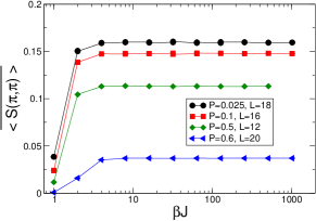
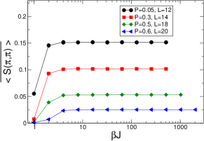
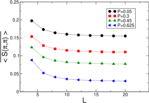
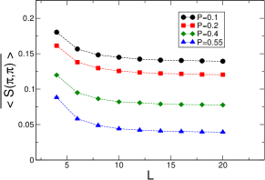
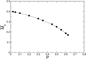
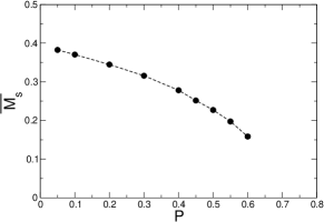
The reach of the ground state values of $\overline{S(\pi,\pi)}$ for several considered $P$ and $L$ is shown in fig. 2 for both the random ladder- and staggered-dimer models. Furthermore, the determination of $\overline{M_{s}}$ is done by extrapolating the related finite volume staggered structure factors to the corresponding bulk results, using a polynomial fit of the form $a_{0}+a_{1}/L+a_{2}/L^{2}+a_{3}/L^{3}$ (The bulk $\overline{M_{s}}$ is given by $\sqrt{a_{0}}$). For both the studied models, the $L$-dependence of $\overline{S(\pi,\pi)}$ for several considered $P$ is depicted in fig. 3. The obtained extrapolating values of $\overline{M_{s}}$ are shown in fig. 4.

Figure 3: $L$ dependence of the staggered structure factors $\overline{S(\pi,\pi)}$, at several considered values of $P$, for both the random ladder- (top panel) and staggered-dimer (bottom panel) models. The dashed lines are added to guide the eye.

Figure 4: $\overline{M_{s}}$ as functions of the considered values of $P$ for both the studied models. While the top panel is for the random ladder-dimer model, the results of $\overline{M_{s}}$ for the random staggered-dimer model is depicted in the bottom panel. The dashed lines are added to guide the eye.

III.2 The determination of $\overline{T_{N}}$

Figure 5: $(\overline{\rho_{s}}/\overline{J})L$ as functions of $T/J$ for $L=$12, 16, 20, 24, 28, 32, and 36 for both the studied models. $J$ is 1.0 in our calculations. While the top panel is for the random ladder-dimer model with $P=0.3$, the results of $(\overline{\rho_{s}}/\overline{J})L$ for the random staggered-dimer model with $P=0.05$ is depicted in the bottom panel. The dashed lines are added to guide the eye.

Figure 6: $\overline{Q_{2}}$ as functions of $T/J$ for $L=$12, 16, 20, 24, 28, 32, and 36 for both the studied models. $J$ is 1.0 in our calculations. While the top panel is for the random ladder-dimer model with $P=0.5$, the results of $Q_{2}$ for the random staggered-dimer model with $P=0.2$ is depicted in the bottom panel. The dashed lines are added to guide the eye.

Figure 7: $\overline{M_{s}/}\sqrt{3}$ as functions of $T/J$ for the random ladder-dimer model with $P=0.05$ (top panel) and $P=0.55$ (bottom panel). $J$ is 1.0 in our calculations. The data points are determined with a up to third order polynomial formula in $1/L$ and the quoted errors are estimated directly from the fits. The solid lines are obtained using the results of the fits (leading singular behaviour ansatz).

Figure 8: $\overline{M_{s}/}\sqrt{3}$ as functions of $T/J$ for the random staggered-dimer model with $P=0.1$ (top panel) and $P=0.4$ (bottom panel). $J$ is 1.0 in our calculations. The data points are determined with a up to third order polynomial formula in $1/L$ and the quoted errors are estimated directly from the fits. The solid lines are obtained using the results of the fits (leading singular behaviour ansatz).

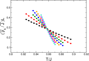
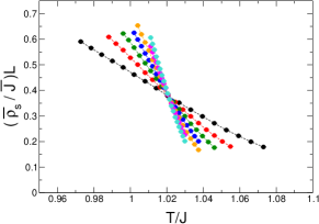
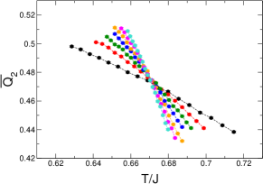
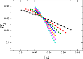
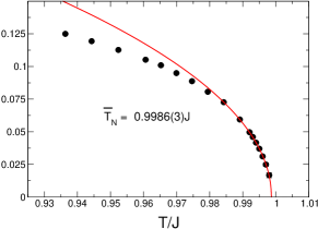
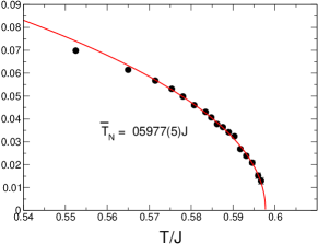
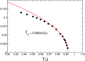
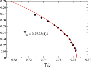
The employed observables for calculating $\overline{T_{N}}$ are $(\overline{\rho_{s}}/\overline{J})L$ as well as $\overline{Q_{2}}$. Notice a constraint standard finite-size scaling ansatz of the form $(1+b_{0}L^{-\omega})(b_{1}+b_{2}tL^{1/\nu}+b_{3}(tL^{1/\nu})^{2}+...$) (or $b_{1}+b_{2}tL^{1/\nu}+b_{3}(tL^{1/\nu})^{2}+...$ in some cases), up to fourth order in $tL^{1/\nu}$, is used to fit the data. Here $b_{i}$ for $i=0,1,2,...$ are some constants and $t=\frac{T-\overline{T_{N}}}{\overline{T_{N}}}$. It has been demonstrated in Ref. Kao14 ; Kao14.1 that such an analysis procedure leads to accurate determination of $\overline{T_{N}}$. The data of $(\overline{\rho_{s}}/\overline{J})L$ for the random ladder-dimer model with $P=0.3$ (top panel) and the random staggered-dimer model with $P=0.05$ (bottom panel) are shown in fig. 5. The values of $\overline{T_{N}}$ obtained from $(\overline{\rho_{s}}/\overline{J})L$ are listed in table 1. Furthermore, the quoted errors appearing in table 1 are conservatively estimated, based on the standard deviations obtained from a bootstrap method used for the fits. Finally, applying a similar analysis to $\overline{Q_{2}}$ leads to consistent results of $\overline{T_{N}}$ with those in table 1. Data points of $\overline{Q_{2}}$ for the random ladder-dimer model with $P=0.5$ and the random staggered-dimer model with $P=0.2$ are presented in fig. 6. In additional to the method of finite-size scaling, $T_{N}$ can also be calculated by studying the singular behaviour of $M_{s}$ when approaching $T_{N}$ from $T\leq T_{N}$. We have performed such investigation for the random ladder-dimer (staggered-dimer) model with $P=0.05,0.55$ ($P=0.1,0.4$). The obtained results of $\overline{T_{N}}$ are in remarkable agreement with those shown in table 1. See figs. 7 and 8 for the details.

$P$		$\overline{T_{N}}/J$		$P$		$\overline{T_{N}}/J$
0.025		1.01030(48)		0.05		1.02030(53)
0.05		0.99909(52)		0.1		0.99308(48)
0.1		0.97550(40)		0.2		0.93097(49)
0.2		0.92208(40)		0.3		0.85645(44)
0.3		0.85703(50)		0.4		0.76297(53)
0.35		0.81891(39)		0.45		0.70586(66)
0.45		0.72636(39)		0.5		0.63896(56)
0.5		0.66832(44)		0.55		0.55730(21)
0.55		0.59868(62)		0.6		0.44937(31)
0.6		0.51146(32)
0.625		0.45649(28)

Table 1: Numerical values of $\overline{T_{N}}/J$ determined from the observable $(\overline{\rho_{s}}/\overline{J})L$ for various $P$. $J$ is 1.0 in our calculations. The first two columns and the last two columns are associated with the random ladder- and staggered-dimer models, respectively.

III.3 The determination of $\overline{T^{\star}}$

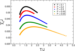
In additional to the universal relation between $T_{N}/\overline{J}$ and $M_{s}$, it is demonstrated in Ref. Jin12 that there exists a universal connection between the quantities $T_{N}/T^{\star}$ and $M_{s}$ as well. Here $T^{\star}$ is the temperature where peak of the uniform susceptibility $\chi_{u}$ ($\chi_{u}=\langle\frac{\beta}{L^{3}}(\sum_{i}S^{z}_{i})^{2}\rangle$), as a function of the temperatures, takes place. For both the studied models, the values of $\overline{T^{\star}}$ for the considered $P$ are estimated from the related data of $L=12$ and $L=24$. The numerical values of $\overline{\chi_{u}}$ as functions of $T/J$ for some values of $P$ and $L=12$ are shown in fig. 9.

Figure 9: $\overline{\chi_{u}}$ of the random ladder-dimer model as functions of $T/J$ for some values of $P$ and $L=12$. $J$ is 1.0 in our calculations.

Figure 10: $\overline{T_{N}}$ as functions of $\overline{M_{s}}$ for both the considered models with the introduced randomness.

Figure 11: Universal behaviour of $\overline{T_{N}}/\overline{J}$ as functions of $\overline{M_{s}}$ for the considered models with the introduced randomness.

III.4 The universal relations

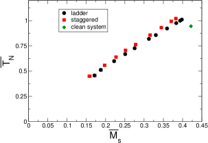
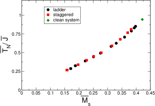
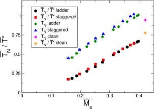
After having obtained $\overline{T_{N}}$, $\overline{J}$, $\overline{M_{s}}$, and $\overline{T^{\star}}$, as a first step to examine whether universal relations, as those established for regular dimerized systems, would appear for the considered models with the employed randomness, we study $\overline{T_{N}}$ as functions of $\overline{M_{s}}$ for both models. The results are shown in fig. 10. As one can see in fig. 10, no clear signal of a universal relation is found in the figure. Remarkably, if the quantity $\overline{T_{N}}/\overline{J}$ is investigated as functions of $\overline{M_{s}}$, then indeed the data points of both models fall on top of a universal curve. The result is demonstrated in fig. 11. Similarly, a universal behaviour between $\overline{T_{N}}/\overline{T^{\star}}$ and $\overline{M_{s}}$ is observed as well (fig. 12).

Figure 12: Universal behaviour of $\overline{T_{N}}/\overline{T^{\star}}$ as functions of $\overline{M_{s}}$ for the considered models with the introduced randomness. The corresponding results of $\overline{T_{N}}$ are shown in the figure as well. The data points of $\overline{T_{N}}/\overline{T^{\star}}$ contain (around) one percent uncertainties due to the errors of $\overline{T^{\star}}$.

IV Discussions and Conclusions

Inspired by the universal relations between the Néel temperature $T_{N}$ and the staggered magnetization density $M_{s}$ for the clean 3D dimerized systems, in this work we study these universal behaviour of $T_{N}$ and $M_{s}$ for a class of 3D random-exchange quantum Heisenberg models. A notable finding here is that these universal properties are even valid for the considered models with the introduced randomness. Our results indicate that the scope of the validity of these universal properties for 3D quantum antiferromagnets is very general. One interesting question is to examine whether the data points obtained with other values of $D$ will fall on top of the universal curves shown in figs. 11 and 12. Our preliminary results related to $\overline{T_{N}}/\overline{J}$ and $\overline{M_{s}}$ show that this is not the case. In addition, the data points associated with clean dimerized ladder model do not form a universal curve with those data points presented in fig. 11. As a result, these universal properties are valid within individual categories, such as the models in fig. 1 with $D=0.5$ which are investigated in detail here. Nevertheless, it is remarkable that the universal relations originally observed for the clean models persist even for systems with randomness.

References

- (1) S. Chakravarty, B. I. Halperin, and D. R. Nelson, Phys. Rev. Lett. 60, 1057 (1988).
- (2) F. D. M. Haldane, Phys. Rev. Lett. 61, 1029 (1988).
- (3) J. D. Reger and A. P. Young, Phys. Rev. B 37, R5978 (1988).
- (4) S. Chakravarty, B. I. Halperin, and D. R. Nelson, Phys. Rev. B 39, 2344 (1989).
- (5) R. R. P. Singh, Phys. Rev. B 39, 9760 (1989).
- (6) R. R. P. Singh, Phys. Rev. B 41, 4873 (1990).
- (7) W. H. Zheng, J. Oitmaa, and C. J. Hamer, Phys. Rev. B 43, 8321 (1991).
- (8) A. V. Chubukov, S. Sachdev, and J. Ye, Phys. Rev. B 49, 11919 (1994).
- (9) J. Oitmaa, C. J. Hamer, and Zheng Weihong, Phys. Rev. B 50, 3877 (1994).
- (10) M. Troyer, H. Kantani, and K. Ueda, Phys. Rev. Lett. 76, 3822 (1996).
- (11) B. B. Beard and U.-J. Wiese, Phys. Rev. Lett. 77, 5130 (1996).
- (12) A. W. Sandvik, Phys. Rev. B (1997).
- (13) Munehisa Matsumoto, Chitoshi Yasuda, Synge Todo, and Hajime Takayama, Phys. Rev. B 65, 014407 (2002).
- (14) L. Wang, K. S. D. Beach, and A. W. Sandvik, Phys. Rev. B 73, 014431 (2006).
- (15) Kwai-Kong Ng and T. K. Lee, Phys. Rev. Lett. 97, 127204 (2006).
- (16) T. Pardini, R. R. P. Singh, A. Katanin and O. P. Sushkov, Phys. Rev. B 78, 024439 (2008).
- (17) F.-J. Jiang, F. Kämpfer, and M. Nyfeler, Phys. Rev. B 80, 033104 (2009).
- (18) S. Sachdev, C. Buragohain, and M. Vojta, Science 286, 2479 (1999).
- (19) M. Vojta, C. Buragohain, and S. Sachdev, Phys. Rev. B 61, 15152 (2000).
- (20) S. Sachdev, M. Troyer, and M. Vojta, Phys. Rev. Lett. 86, 2617 (2001).
- (21) M. Troyer, Prog. Theor. Phys. Supp. 145, 326 (2002).
- (22) S. Sachdev and M. Vojta, Phys. Rev. B 68, 064419 (2003).
- (23) O. P. Sushkov, Phys. Rev. B 68, 094426 (2003).
- (24) K. H. Höglund and A. W. Sandvik, Phys. Rev. Lett. 91, 077204 (2003).
- (25) K. H. Höglund and A. W. Sandvik, Phys. Rev. B 70, 024406 (2004).
- (26) K. H. Höglund, A. W. Sandvik, and S. Sachdev, Phys. Rev. Lett. 98, 087203 (2007).
- (27) K. H. Höglund and A. W. Sandvik, Phys. Rev. Lett. 99, 027205 (2007).
- (28) A. W. Sandvik and M. Vekic, Phys. Rev. Lett. 74, 1226 (1995).
- (29) R. Melin, Y.-C. Lin, P. Lajko, H. Rieger, and F. Iglói, Phys. Rev. B 65, 104415 (2002).
- (30) Y. C. Lin, H. Rieger, and F. Iglói, Phys. Rev. B 68, 024424 (2003).
- (31) Nicolas Laflorencie, Stefen Wessel, Andreas Läuchli, and Heiko Rieger, Phys. Reiv B 73, 060403(R) (2006).
- (32) Y. C. Lin, H. Rieger, N. Laflorencie, and F. Iglói, Phys. Rev. B 74, 024427 (2006).
- (33) T. Vojta, J. Low Temp. Phys. 161, 299 (2010).
- (34) N. Cavadini, G. Heigold, W. Henggeler, A. Furrer, H.-U. Güdel, K. Krämer, and H. Mutka, Phys. Rev. B 63, 172414 (2001).
- (35) Ch. Rüegg, N.Cavadini, A. Furrer, H.-U. Güdel, K. Krämer, H. Mutka, A. Wildes, K. Habicht, and P. Vorderwisch, Nature (London) 423, 62, (2003).
- (36) Ch. Rüegg et al., Phys. Rev. Lett. 100, 205701 (2008).
- (37) J. Oitmaa and Weihong Zheng, J. Phys.: Condens. Matter 16, 8653 (2004).
- (38) O. Nohadani, S. Wessel, and S. Haas, Phys. Rev. B 72, 024440 (2005).
- (39) Y. Kulik, and O. P. Sushkov, Phys. Rev. B 84, 134418 (2011).
- (40) J. Oitmaa, Y. Kulik, and O. P. Sushkov, Phys. Rev. B 85, 144431 (2012).
- (41) S. Jin and A. W. Sandvik, Phys. Rev. B 85, 020409(R) (2012).
- (42) M.-T. Kao and F.-J. Jiang, Eur. Phy. J. B, (2013) 86: 419.
- (43) P. Merchant, B. Normand, K. W. Krämer, M. Boehm, D. F. McMorrow, and Ch. Rüegger, Nature physics 10, 373-379 (2014).
- (44) M.-T. Kao, D.-R. Tan, and F.-J. Jiang, unpublished.
- (45) M.-T. Kao, PhD dissertation (2014), National Taiwan Normal University, Taipei, Taiwan.
- (46) Nvsen Ma, Anders W. Sandvik, and Dao-Xin Yao, Phys. Rev. B 90, 104425 (2014).
- (47) A. W. Sandvik, Phys. Rev. B 66, R14157 (1999).
- (48) A. W. Sandvik, Phys. Rev. B 66, 024418 (2002).