A Cascadic Multigrid Method for GPE Problem

Abstract

A cascadic multigrid method is proposed for the GPE problem based on the multilevel correction scheme. With this new scheme, the ground state eigenvalue problem on the finest space can be solved by smoothing steps on a series of multilevel finite element spaces and some nonlinear eigenvalue problem solving on a very low-dimensional space. Choosing the appropriate sequence of finite element spaces and the number of smoothing steps, the optimal convergence rate with the optimal computational work can be arrived. Some numerical experiments are presented to validate our theoretical analysis. Keywords. Bose-Einstein condensation; Gross-Pitaevskii equation; multilevel correction; cascadic multigrid; nonlinear eigenvalue problem; finite element method.

AMS subject classifications. 65N30, 65N25, 65L15, 65B99.

1 Introduction

The aim of this paper is to design a cascadic type multigrid finite element method for solving Gross-Pitaevskii equation (GPE) which is a time independent Schrödinger equation. The finite element method for GPE problem and general semilinear eigenvalue problem has been investigated by [3, 15]. The corresponding error estimates are also given.

Recently, a type of multilevel correction method is proposed to solve eigenvalue problems in [6, 12, 13]. In this multilevel correction scheme, the solution of eigenvalue problem on the final level mesh can be reduced to a series of solutions of boundary value problems on the multilevel meshes and a series of solutions of the eigenvalue problem in a very low-dimensional space. Therefore, the cost of computation work can be reduced largely. A multigrid method for the GPE has been proposed in [14] where a superapproximate property is founded. Therefore, the aim of this paper is to construct a cascadic multigrid method to solve the ground state solution of Bose-Eienstein condensates (BEC). The cascadic multigrid method for second order elliptic eigenvalue problem is given in [5]. This method transforms the eigenvalue problem solving to a series of smoothing iteration steps on the sequence of meshes and eigenvalue problem solving on the coarsest mesh by the multilevel correction method. Similarly to the cascadic multigrid for the boundary value problem [2, 9], we only do the smoothing steps for the involved boundary value problems by using the previous eigenpair approximation as the start value and the numbers of smoothing iteration steps need to be increased in the coarse levels. The order of the algebraic error for the final eigenpair approximation can arrive the same as the discretization error of the finite element method by organizing suitable numbers of smoothing iteration steps in different levels. The nonlinear eigenvalue problems on a very low-dimensional space are solved by self-consistent iteration or Newton type iteration which reduces the nonlinear eigenvalue problem to a series of linear ones.

The rest of this paper is organized as follows. In the next section, we introduce the finite element method for the ground state solution of BEC. A cascadic multigrid method for solving the non-dimensionalized GPE is presented and analyzed in Section 3. In Section 4, some numerical tests are presented to validate our theoretical analysis. Some concluding remarks are given in the last section.

2 Finite element method for GPE problem

This section is devoted to introducing some notation and the finite element method for the GPE problem. In this paper, we shall use the standard notation for Sobolev spaces $W^{s,p}(\Omega)$ and their associated norms and semi-norms (cf. [1]). For $p=2$, we denote $H^{s}(\Omega)=W^{s,2}(\Omega)$ and $H_{0}^{1}(\Omega)=\{v\in H^{1}(\Omega):\ v|_{\partial\Omega}=0\}$, where $v|_{\Omega}=0$ is in the sense of trace, $\|\cdot\|_{s,\Omega}=\|\cdot\|_{s,2,\Omega}$. The letter $C$ (with or without subscripts) denotes a generic positive constant which may be different at its different occurrences through the paper.

For simplicity, we consider the following non-dimensionalized GPE problem: Find $(\lambda,u)$ such that

$$\left\{\begin{array}[]{rcl}-\Delta u+Wu+\zeta|u|^{2}u&=&\lambda u,\quad{\rm in}\ \Omega,\\ u&=&0,\ \ \quad{\rm on}\ \partial\Omega,\\ \int_{\Omega}|u|^{2}d\Omega&=&1,\end{array}\right.$$ (2.1)

where $\Omega\subset\mathcal{R}^{d}$ $(d=2,3)$ is a bounded domain with Lipschitz boundary $\partial\Omega$, $\zeta$ is some positive constant and $W(x)=\gamma_{1}x_{1}^{2}+\cdots+\gamma_{d}x_{d}^{2}\geq 0$ with $\gamma_{1},\cdots,\gamma_{d}>0$.

In order to use the finite element method to solve the eigenvalue problem (2.1), we need to define the corresponding variational form as follows: Find $(\lambda,u)\in\mathcal{R}\times V$ such that $b(u,u)=1$ and

$$a(u,v) = \lambda b(u,v),\quad\forall v\in V,$$ (2.2)

where $V:=H_{0}^{1}(\Omega)$ and

$$a(u,v):=\int_{\Omega}\big{(}\nabla u\nabla v+Wuv+\zeta|u|^{2}uv\big{)}d\Omega,\ \ b(u,v):=\int_{\Omega}uvd\Omega.$$ (2.3)

The existence, uniqueness and simplicity of the smallest eigenpair of eigenvalue problem (2.2) have been given in [3].

To simplify the notation, we also define $H^{1}(\Omega)$ inner-product $\widehat{a}(\cdot,\cdot)$ as

$$\widehat{a}(w,v):=\int_{\Omega}\nabla w\nabla vd\Omega,\ \ \forall w,v\in V.$$ (2.4)

Now, let us define the finite element approximations of the problem (2.2). First we generate a shape-regular decomposition of the computing domain $\Omega\subset\mathcal{R}^{d}\ (d=2,3)$ into triangles or rectangles for $d=2$ (tetrahedrons or hexahedrons for $d=3$). The diameter of a cell $K\in\mathcal{T}_{h}$ is denoted by $h_{K}$ and the mesh size $h$ describes the maximum diameter of all cells $K\in\mathcal{T}_{h}$. Based on the mesh $\mathcal{T}_{h}$, we can construct a finite element space denoted by $V_{h}\subset V$. For simplicity, we set $V_{h}$ as the linear finite element space which is defined as follows

$$V_{h}=\big{\{}v_{h}\in C(\Omega)\ \big{|}\ v_{h}|_{K}\in\mathcal{P}_{1},\ \ \forall K\in\mathcal{T}_{h}\big{\}},$$ (2.5)

where $\mathcal{P}_{1}$ denotes the linear function space.

The standard finite element scheme for eigenvalue problem (2.2) is: Find $(\bar{\lambda}_{h},\bar{u}_{h})\in\mathcal{R}\times V_{h}$ such that $b(\bar{u}_{h},\bar{u}_{h})=1$ and

$$a(\bar{u}_{h},v_{h}) = \bar{\lambda}_{h}b(\bar{u}_{h},v_{h}),\quad\ \ \ \forall v_{h}\in V_{h}.$$ (2.6)

Then we define

$$\delta_{h}(u):=\inf_{v_{h}\in V_{h}}\|u-v_{h}\|_{1}.$$ (2.7)

Lemma 2.1.

([3, Theorem 1]) There exists $h_{0}>0$, such that for all $0<h<h_{0}$, the smallest eigenpair approximation $(\bar{\lambda}_{h},\bar{u}_{h})$ of (2.6) having the following error estimates

$$\|u-\bar{u}_{h}\|_{1} \leq C\delta_{h}(u),$$ (2.8)

$$\|u-\bar{u}_{h}\|_{0} \leq C\eta_{a}(V_{h})\|u-\bar{u}_{h}\|_{1}\leq C\eta_{a}(V_{h})\delta_{h}(u),$$ (2.9)

$$|\lambda-\bar{\lambda}_{h}| \leq C\big{(}\|u-\bar{u}_{h}\|_{1}^{2}+\|u-\bar{u}_{h}\|_{0}\big{)}\leq C\eta_{a}(V_{h})\delta_{h}(u),$$ (2.10)

where $\eta_{a}(V_{h})$ is defined as follows

$$\eta_{a}(V_{h})=\sup_{f\in L^{2}(\Omega),\|f\|_{0}=1}\inf_{v_{h}\in V_{h}}\|Tf-v_{h}\|_{1}$$ (2.11)

with the operator $T$ being defined as follows: Find $Tf\in u^{\bot}$ such that

$$a(Tf,v)+2\big{(}\zeta|u|^{2}(Tf),v\big{)}-\big{(}\lambda(Tf),v\big{)}=(f,v),\ \ \forall v\in u^{\bot},$$

where $u^{\bot}=\{v\in H_{0}^{1}(\Omega):|\int_{\Omega}uvd\Omega=0\}$. Here we use the fact that $\delta_{h}(u)\leq C\eta_{a}(V_{h})$.

3 Cascadic multigrid method for GPE

Recently, a multilevel correction scheme is introduced in [6, 12, 13] for solving Laplace eigenvalue problems. Based on their involved idea, we propose a type of cascadic multigrid method for GPE problem (2.2) in this paper. The main idea in this method is to approximate the underlying boundary value problems on each level by some simple smoothing iteration steps. In order to describe the cascadic multigrid method, we first introduce the sequence of finite element spaces and the properties of the concerned smoothers.

In order to design multigrid scheme, we first generate a coarse mesh $\mathcal{T}_{H}$ with the mesh size $H$ and the coarse linear finite element space $V_{H}$ is defined on it. Then we define a sequence of triangulations $\mathcal{T}_{h_{k}}$ of $\Omega\subset\mathcal{R}^{d}$ determined as follows. Suppose $\mathcal{T}_{h_{1}}$ (produced from $\mathcal{T}_{H}$ by regular refinements) is given and let $\mathcal{T}_{h_{k}}$ be obtained from $\mathcal{T}_{h_{k-1}}$ via one regular refinement step (produce $\beta^{d}$ subelements) such that

$$h_{k}\approx\frac{1}{\beta}h_{k-1},$$ (3.1)

where the positive number $\beta$ denotes the refinement index and larger than $1$ (always equals $2$). Based on this sequence of meshes, we construct the corresponding nested linear finite element spaces such that

$$V_{H}\subseteq V_{h_{1}}\subset V_{h_{2}}\subset\cdots\subset V_{h_{n}}.$$ (3.2)

The sequence of finite element spaces $V_{h_{1}}\subset V_{h_{2}}\subset\cdots\subset V_{h_{n}}$ and the finite element space $V_{H}$ have the following relations of approximation accuracy

$$\eta_{a}(V_{H})\gtrsim\delta_{h_{1}}(u),\ \ \ \ \delta_{h_{k}}(u)\approx\frac{1}{\beta}\delta_{h_{k-1}}(u),\ \ \ k=2,\cdots,n.$$ (3.3)

In fact, since the ground eigenvalue $\lambda$ of (2.2) is simple (see [3]) and the computing domain is convex, we have the following estimates

$$\eta_{a}(V_{H})\approx H,\ \ \ \ \eta_{a}(V_{h_{k}})\approx h_{k}\ \ \ \ {\rm and}\ \ \ \ \delta_{h_{k}}(u)\approx h_{k},\ \ \ \ k=1,\cdots,n.$$ (3.4)

Remark 3.1.

The relation (3.3) is reasonable since we can choose $\delta_{h_{k}}(u)=h_{k}\ (k=1,\cdots,n)$. Always the upper bound of the estimate $\delta_{h_{k}}(u)\lesssim h_{k}$ holds. Recently, we also obtain the lower bound result $\delta_{h_{k}}(u)\gtrsim h_{k}$ (c.f. [7]).

For generality, we introduce a smoothing operator $S_{h}:V_{h}\rightarrow V_{h}$ which satisfies the following estimates

$$\left\{\begin{array}[]{rcl}\|S_{h}^{m}w_{h}\|_{1}&\leq&\frac{C}{m^{\alpha}}\frac{1}{h}\|w_{h}\|_{0},\\ \|S_{h}^{m}w_{h}\|_{1}&\leq&\|w_{h}\|_{1},\\ \|S_{h}^{m}(w_{h}+v_{h})\|_{1}&\leq&\|S_{h}^{m}w_{h}\|_{1}+\|S_{h}^{m}v_{h}\|_{1},\end{array}\right.$$ (3.5)

where $C$ is a constant independent of $h$ and $\alpha$ is some positive number depending on the choice of smoother. It is proved in [4, 8, 11] that the symmetric Gauss-Seidel, the SSOR, the damped Jacobi and the Richardson iteration are smoothers in the sense of (3.5) with parameter $\alpha=1/2$ and the conjugate-gradient iteration is the smoother with $\alpha=1$ (cf. [9, 10]).

Then we define the following notation

$$w_{h}={\it Smooth}(V_{h},f,\xi_{h},m,S_{h})$$ (3.6)

as the smoothing process for the following boundary value problem

$$\widehat{a}(u_{h},v_{h})=b(f,v_{h}),\ \ \ \ \forall v_{h}\in V_{h},$$ (3.7)

where $\xi_{h}$ denote the initial value of the smoothing process, $S_{h}$ denote the chosen smoothing operator, $m$ the number of the iteration steps and $w_{h}$ is the output of the smoothing process.

Now, we come to introduce the cascadic multigrid method for the eigenvalue problem (2.2). Assume we have obtained an eigenpair approximations $(\lambda^{h_{k}},u^{h_{k}})\in\mathcal{R}\times V_{h_{k}}$. We design the following cascadic type one correction step to improve the accuracy of the current eigenpair approximation $(\lambda^{h_{k}},u^{h_{k}})\in\mathcal{R}\times V_{h_{k}}$.

Algorithm 3.1.

Cascadic type of One Correction Step

1. Define the following auxiliary source problem: Find $\widehat{u}^{h_{k+1}}\in V_{h_{k+1}}$ such that

   $$\widehat{a}(\widehat{u}^{h_{k+1}},v_{h_{k+1}})=\lambda^{h_{k}}b(u^{h_{k}},v_{h_{k+1}})$$

   $$\quad\quad\quad-\big{(}(W+\zeta|u^{h_{k}}|^{2})u^{h_{k}},v_{h_{k+1}}\big{)},\ \ \forall v_{h_{k+1}}\in V_{h_{k+1}}.$$ (3.8)

   Perform the smoothing process (3.6) to obtain a new eigenfuction approximation $\widetilde{u}^{h_{k+1}}\in V_{h_{k+1}}$ by

   $$\widetilde{u}^{h_{k+1}}={\it Smooth}(V_{h_{k+1}},\lambda^{h_{k}}u^{h_{k}}-(W+\zeta|u^{h_{k}}|^{2})u^{h_{k}},u^{h_{k}},m_{k+1},S_{h_{k+1}}).$$ (3.9)

2. Define a new finite element space $V_{H}^{h_{k+1}}=V_{H}+{\rm span}\{\widetilde{u}^{h_{k+1}}\}$ and solve the following eigenvalue problem: Find $(\lambda^{h_{k+1}},u^{h_{k+1}})\in\mathcal{R}\times V_{H}^{h_{k+1}}$ such that
   $b(u^{h_{k+1}},u^{h_{k+1}})=1$ and

   $$a(u^{h_{k+1}},v_{H}^{h_{k+1}})=\lambda^{h_{k+1}}b(u^{h_{k+1}},v_{H}^{h_{k+1}}),\ \ \ \ \ \forall v_{H}^{h_{k+1}}\in V_{H}^{h_{k+1}}.$$ (3.10)

Summarize the above two steps by defining

$$(\lambda^{h_{k+1}},u^{h_{k+1}})={\it SmoothCorrection}(V_{H},V_{h_{k+1}},\lambda^{h_{k}},u^{h_{k}},m_{k+1},S_{h_{k+1}}).$$

Based on the above algorithm, i.e., the cascadic type of one correction step, we can construct a cascadic multigrid method for GPE as follows:

Algorithm 3.2.

GPE Cascadic Multigrid Method

1. Solve the following GPE problem in the initial finite element space $V_{h_{1}}$: Find $(\lambda^{h_{1}},u^{h_{1}})\in\mathcal{R}\times V_{h_{1}}$ such that

   $$a(u^{h_{1}},v_{h_{1}})=\lambda^{h_{1}}b(u^{h_{1}},v_{h_{1}}),\quad\forall v_{h_{1}}\in V_{h_{1}}.$$

2. For $k=1,\cdots,n-1$, do the following iteration

   $$(\lambda^{h_{k+1}},u^{h_{k+1}})={\it SmoothCorrection}(V_{H},V_{h_{k+1}},\lambda^{h_{k}},u^{h_{k}},m_{k+1},S_{h_{k+1}}).$$

   End Do

Finally, we obtain an eigenpair approximation $(\lambda^{h_{n}},u^{h_{n}})\in\mathcal{R}\times V_{h_{n}}$.

In order to analyze the convergence of Algorithm 3.2, we introduce an auxiliary algorithm and then show its superapproximate property. Similarly, assume we have obtained an eigenpair approximations $(\widetilde{\lambda}_{h_{k}},\widetilde{u}_{h_{k}})\in\mathcal{R}\times V_{h_{k}}$. The following auxiliary one correction step is defined as follows.

Algorithm 3.3.

Auxiliary One Correction Step

1. Solve the following auxiliary source problem: Find $\widehat{u}_{h_{k+1}}\in V_{h_{k+1}}$ such that

   $$\widehat{a}(\widehat{u}_{h_{k+1}},v_{h_{k+1}})=\widetilde{\lambda}_{h_{k}}b(\widetilde{u}_{h_{k}},v_{h_{k+1}})$$

   $$\quad\quad\quad-\big{(}\big{(}W+\zeta|\widetilde{u}_{h_{k}}|^{2}\big{)}\widetilde{u}_{h_{k}},v_{h_{k+1}}\big{)},\ \ \forall v_{h_{k+1}}\in V_{h_{k+1}}.$$ (3.11)

2. Define a new finite element space $\widetilde{V}_{H,h_{k+1}}=V_{H}+{\rm span}\{\widehat{u}_{h_{k+1}}\}+{\rm span}\{\widetilde{u}^{h_{k+1}}\}$ and solve the following eigenvalue problem: Find $(\widetilde{\lambda}_{h_{k+1}},\widetilde{u}_{h_{k+1}})\in\mathcal{R}\times\widetilde{V}_{H,h_{k+1}}$ such that $b(\widetilde{u}_{h_{k+1}},\widetilde{u}_{h_{k+1}})=1$ and

   $$a(\widetilde{u}_{h_{k+1}},\widetilde{v}_{H,h_{k+1}})=\widetilde{\lambda}_{h_{k+1}}b(\widetilde{u}_{h_{k+1}},\widetilde{v}_{H,h_{k+1}}),\ \ \ \ \ \forall\widetilde{v}_{H,h_{k+1}}\in\widetilde{V}_{H,h_{k+1}}.$$ (3.12)

Summarize the above two steps by defining

$$(\widetilde{\lambda}_{h_{k+1}},\widetilde{u}_{h_{k+1}})={\it AuxiliaryCorrection}(V_{H},V_{h_{k+1}},\widetilde{\lambda}_{h_{k}},\widetilde{u}_{h_{k}},\widetilde{u}^{h_{k+1}}).$$

Algorithm 3.4.

GPE Auxiliary Multilevel Correction Method

1. Solve the following GPE problem in the initial finite element space $V_{h_{1}}$: Find $(\widetilde{\lambda}_{h_{1}},\widetilde{u}_{h_{1}})\in\mathcal{R}\times V_{h_{1}}$ such that

   $$a(\widetilde{u}_{h_{1}},v_{h_{1}})=\widetilde{\lambda}_{h_{1}}b(\widetilde{u}_{h_{1}},v_{h_{1}}),\quad\forall v_{h_{1}}\in V_{h_{1}}.$$

2. For $k=1,\cdots,n-1$, do the following iteration

   $$(\widetilde{\lambda}_{h_{k+1}},\widetilde{u}_{h_{k+1}})={\it AuxiliaryCorrection}(V_{H},V_{h_{k+1}},\widetilde{\lambda}_{h_{k}},\widetilde{u}_{h_{k}},\widetilde{u}^{h_{k+1}}).$$

   End Do

Finally, we obtain an eigenpair approximation $(\widetilde{\lambda}_{h_{n}},\widetilde{u}_{h_{n}})\in\mathcal{R}\times V_{h_{n}}$.

Before analyzing the convergence of Algorithm 3.2, we show a superapproximate property of $\widetilde{u}_{h_{k}}$ obtained by Algorithm 3.4. The similar result is also analyzed in [14].

Theorem 3.1.

Assume $\widetilde{u}_{h_{k}}$ ($k=1,\cdots,n$) are obtained by Algorithm 3.4 and $\bar{u}_{h_{k}}$ ($k=1,\cdots,n$) the standard finite element solution in $V_{h_{k}}$. If the sequence of finite element spaces $V_{h_{1}},\cdots,V_{h_{n}}$ and the coarse finite element space $V_{H}$ satisfy the following condition

$$C\eta_{a}(V_{H})\beta^{2}<1,$$ (3.13)

the following estimate holds

$$\|\bar{u}_{h_{k}}-\widetilde{u}_{h_{k}}\|_{1}\leq C\eta_{a}(V_{h_{k}})\delta_{h_{k}}(u),\ \ \ \ \ \ \ k=1,\cdots,n,$$ (3.14)

and

$$\|\bar{u}_{h_{k}}-\widetilde{u}_{h_{k}}\|_{0}\leq C\eta_{a}(V_{h_{k}})\delta_{h_{k}}(u),\ \ \ \ \ \ \ k=1,\cdots,n,$$ (3.15)

where $C$ is a constant only depending on the eigenvalue $\lambda$. The eigenvalue approximations $\widetilde{\lambda}_{h_{k}}$ and $\bar{\lambda}_{h_{k}}$ have the following estimates

$$\big{|}\bar{\lambda}_{h_{k}}-\widetilde{\lambda}_{h_{k}}\big{|}\leq C\eta_{a}(V_{h_{k}})\delta_{h_{k}}(u),\ \ \ \ \ \ \ k=1,2,\cdots,n.$$ (3.16)

Proof.

Define $\varepsilon_{h_{k}}:=|\widetilde{\lambda}_{h_{k}}-\bar{\lambda}_{h_{k}}|+\|\widetilde{u}_{h_{k}}-\bar{u}_{h_{k}}\|_{0},\ k=1,2,\cdots,n$. And it is obvious that $\varepsilon_{h_{1}}=0$. From (2.6) and (1), we have

$$\widehat{a}(\bar{u}_{h_{k+1}}-\widehat{u}_{h_{k+1}},v_{h_{k+1}})$$

$$= b(\bar{\lambda}_{h_{k+1}}\bar{u}_{h_{k+1}}-\widetilde{\lambda}_{h_{k}}\widetilde{u}_{h_{k}},v_{h_{k+1}})$$

$$+\big{(}\big{(}W+\zeta|u^{h_{k}}|^{2}\big{)}u^{h_{k}}-\big{(}W+\zeta|\bar{u}_{h_{k+1}}|^{2}\big{)}\bar{u}_{h_{k+1}},v_{h_{k+1}}\big{)}$$

$$\leq C\big{(}\|\bar{\lambda}_{h_{k+1}}\bar{u}_{h_{k+1}}-\widetilde{\lambda}_{h_{k}}\widetilde{u}_{h_{k}}\|_{0}\|v_{h_{k+1}}\|_{1}$$

$$\quad\quad+\|\bar{u}_{h_{k+1}}-\widetilde{u}_{h_{k}}\|_{0}\big{(}\|\bar{u}_{h_{k+1}}\|_{0,6,\Omega}^{2}+\|\widetilde{u}_{h_{k}}\|_{0,6,\Omega}^{2}\big{)}\|v_{h_{k+1}}\|_{1}\big{)}$$

$$\leq C\big{(}\|\bar{\lambda}_{h_{k+1}}\bar{u}_{h_{k+1}}-\bar{\lambda}_{h_{k}}\bar{u}_{h_{k}}\|_{0}+\|\bar{\lambda}_{h_{k}}\bar{u}_{h_{k}}-\widetilde{\lambda}_{h_{k}}\widetilde{u}_{h_{k}}\|_{0}$$

$$+\big{(}\|\bar{u}_{h_{k+1}}-\bar{u}_{h_{k}}\|_{0}+\|\bar{u}_{h_{k}}-\widetilde{u}_{h_{k}}\|_{0}\big{)}\big{(}\|\bar{u}_{h_{k+1}}\|_{1}^{2}+\|\widetilde{u}_{h_{k}}\|_{1}^{2}\big{)}\big{)}\|v_{h_{k+1}}\|_{1}$$

$$\leq C\big{(}|\bar{\lambda}_{h_{k+1}}-\bar{\lambda}_{h_{k}}|+\|\bar{u}_{h_{k+1}}-\bar{u}_{h_{k}}\|_{0}+\varepsilon_{h_{k}}\big{)}\|v_{h_{k+1}}\|_{1}.$$

It leads to the following estimates

$$\|\bar{u}_{h_{k+1}}-\widehat{u}_{h_{k+1}}\|_{1}\leq C\big{(}|\bar{\lambda}_{h_{k+1}}-\bar{\lambda}_{h_{k}}|+\|\bar{u}_{h_{k+1}}-\bar{u}_{h_{k}}\|_{0}+\varepsilon_{h_{k}}\big{)}.$$ (3.17)

Note that the eigenvalue problem (3.12) can be regarded as a finite dimensional subspace approximation of the eigenvalue problem (2.6). Similarly to Lemma 2.1 (see [3]), from the second step in Algorithm 3.3, the following estimate holds

$$\|\bar{u}_{h_{k+1}}-\widetilde{u}_{h_{k+1}}\|_{1}\leq C\inf_{\widetilde{v}_{H,h_{k+1}}\in\widetilde{V}_{H,h_{k+1}}}\|\bar{u}_{h_{k+1}}-\widetilde{v}_{H,h_{k+1}}\|_{1}\leq C\|\bar{u}_{h_{k+1}}-\widehat{u}_{h_{k+1}}\|_{1}.$$ (3.18)

Then combining (3.17) and (3.18) leads to

$$\|\bar{u}_{h_{k+1}}-\widetilde{u}_{h_{k+1}}\|_{1}\leq C\big{(}|\bar{\lambda}_{h_{k+1}}-\bar{\lambda}_{h_{k}}|+\|\bar{u}_{h_{k+1}}-\bar{u}_{h_{k}}\|_{0}+\varepsilon_{h_{k}}\big{)}.$$ (3.19)

From the properties of $V_{h_{k}}\subset V_{h_{k+1}}$, $\widetilde{V}_{H,h_{k}}\subset V_{h_{k}}$, Lemma 2.1 and (3.3), we have

$$\|\bar{u}_{h_{k+1}}-\bar{u}_{h_{k}}\|_{1}\leq C\delta_{h_{k}}(u),\ \ \ \|\bar{u}_{h_{k+1}}-\bar{u}_{h_{k}}\|_{0}\leq C\eta_{a}(V_{h_{k}})\|\bar{u}_{h_{k+1}}-\bar{u}_{h_{k}}\|_{1},$$

$$\big{|}\bar{\lambda}_{h_{k+}}-\bar{\lambda}_{h_{k}}\big{|}\leq C\eta_{a}(V_{h_{k}})\delta_{h_{k}}(u),\ \ \ \|\bar{u}_{h_{k}}-\widetilde{u}_{h_{k}}\|_{0}\leq C\eta_{a}(V_{H})\|\bar{u}_{h_{k}}-\widetilde{u}_{h_{k}}\|_{1},$$

$$\big{|}\bar{\lambda}_{h_{k}}-\widetilde{\lambda}_{h_{k}}\big{|}\leq C\eta_{a}(V_{H})\|\bar{u}_{h_{k}}-\widetilde{u}_{h_{k}}\|_{1}.$$

Substituting above inequalities into (3.19) leads to the following estimates

$$\|\bar{u}_{h_{k+1}}-\widetilde{u}_{h_{k+1}}\|_{1} \leq C\big{(}\eta_{a}(V_{h_{k}})\delta_{h_{k}}(u)+\varepsilon_{h_{k}}\big{)}$$ (3.20)

$$\leq C\big{(}\eta_{a}(V_{h_{k}})\delta_{h_{k}}(u)+\eta_{a}(V_{H})\|\bar{u}_{h_{k}}-\widetilde{u}_{h_{k}}\|_{1}\big{)}.$$

When $k=1$, since $\widetilde{u}_{h_{1}}:=\bar{u}_{h_{1}}$ and $\widetilde{\lambda}_{h_{1}}:=\bar{\lambda}_{h_{1}}$, we have

$$\|\bar{u}_{h_{2}}-\widetilde{u}_{h_{2}}\|_{1}\leq C\eta_{a}(V_{h_{1}})\delta_{h_{1}}(u).$$ (3.21)

Based on (3.3), (3.20), (3.21) and recursive argument, we have the following estimates:

$$\|\bar{u}_{h_{k}}-\widetilde{u}_{h_{k}}\|_{1} \leq C\sum_{j=2}^{k}\big{(}C\eta_{a}(V_{H})\big{)}^{k-j}\eta_{a}(V_{h_{j-1}})\delta_{h_{j-1}}(u)$$ (3.22)

$$\leq C\sum_{j=2}^{k}\big{(}C\eta_{a}(V_{H})\big{)}^{k-j}\beta^{k-j+1}\eta_{a}(V_{h_{k}})\beta^{k-j+1}\delta_{h_{k}}(u)$$

$$\leq C{\beta}^{2}\Big{(}\sum_{j=2}^{k}\big{(}C\eta_{a}(V_{H})\beta^{2}\big{)}^{k-j}\Big{)}\eta_{a}(V_{h_{k}})\delta_{h_{k}}(u)$$

$$\leq \frac{C\beta^{2}}{1-C\beta^{2}\eta_{a}(V_{H})}\eta_{a}(V_{h_{k}})\delta_{h_{k}}(u).$$

Therefore, the desired result (3.14) holds under the condition $C\eta_{a}(V_{H})\beta^{2}<1$. Furthermore, (3.15) and (3.16) can be obtained directly from Lemma 2.1 and the property $\widetilde{V}_{H,h_{k+1}}\subset V_{h_{k+1}}$. ∎

Note that $V_{H}^{h_{k}}\subset\widetilde{V}_{H,h_{k}}$, we can obtain the following estimates which play an important role in our analysis.

Lemma 3.1.

[3, Theorem 1] Let $u^{h_{k}}$, $V_{H}^{h_{k}}$ and $\widetilde{u}_{h_{k}}$, $\widetilde{V}_{H,h_{k}}$ be defined in Algorithms 3.1 and 3.3. Then the following estimates hold:

$$\|u^{h_{k}}-\widetilde{u}_{h_{k}}\|_{1} \leq C\|\widehat{u}_{h_{k}}-\widetilde{u}^{h_{k}}\|_{1},$$ (3.23)

$$\|u^{h_{k}}-\widetilde{u}_{h_{k}}\|_{0} \leq C\eta_{a}(V_{H})\|u^{h_{k}}-\widetilde{u}_{h_{k}}\|_{1},$$ (3.24)

$$|\lambda^{h_{k}}-\widetilde{\lambda}_{h_{k}}| \leq C\eta_{a}(V_{H})\|u^{h_{k}}-\widetilde{u}_{h_{k}}\|_{1}.$$ (3.25)

Proof.

Since $V_{H}^{h_{k}}\subset\widetilde{V}_{H,h_{k}}$, according to (3.10) and (3.12), $u^{h_{k}}$ can be viewed as the spectral projection of $\widetilde{u}_{h_{k}}$. Then from Lemma 2.1 and the definitions of $\widetilde{V}_{H,h_{k}}$ and $V_{H}^{h_{k}}$, we have

$$\|\widetilde{u}_{h_{k}}-u^{h_{k}}\|_{1} \leq C\inf_{v_{H}^{h_{k}}\in V_{H}^{h_{k}}}\|\widetilde{u}_{h_{k}}-v_{H}^{h_{k}}\|_{1}\leq C\inf_{v_{H}^{h_{k}}\in V_{H}^{h_{k}}}\|\widehat{u}_{h_{k}}-v_{H}^{h_{k}}\|_{1}$$ (3.26)

$$\leq C\|\widehat{u}_{h_{k}}-\widetilde{u}^{h_{k}}\|_{1},$$

which is the desired result (3.23).

Similarly, we also have (3.24) by the following argument

$$\|\widetilde{u}_{h_{k}}-u^{h_{k}}\|_{0}\leq C\eta_{a}(V_{H}^{h_{k}})\|\widetilde{u}_{h_{k}}-u^{h_{k}}\|_{1}\leq C\eta_{a}(V_{H})\|\widetilde{u}_{h_{k}}-u^{h_{k}}\|_{1}.$$

Furthermore, (3.25) can be obtained directly from Lemma 2.1 and the proof is complete. ∎

Remark 3.2.

Since $V_{H}\subset V_{H}^{h_{k}}$ and $V_{H}\subset\widetilde{V}_{H,h_{k}}$, from Lemma 2.1, we have

$$\|u^{h_{k}}-\widetilde{u}_{h_{k}}\|_{1}\leq\|u^{h_{k}}-u\|_{1}+\|u-\widetilde{u}_{h_{k}}\|_{1}\leq C\delta_{H}(u).$$ (3.27)

Now, we come to give error estimates for Algorithm 3.2.

Theorem 3.2.

Assume the eigenpair approximation $(\lambda^{h_{n}},u^{h_{n}})$ is obtained by Algorithm 3.2, $(\widetilde{\lambda}_{h_{n}},\widetilde{u}_{h_{n}})$ is obtained by Algorithm 3.4 and the smoother selected in each level $V_{h_{k}}$ satisfy the smoothing property (3.5) for $k=1,\cdots,n$. Under the conditions of Theorem 3.1, we have the following estimate

$$\|\widetilde{u}_{h_{n}}-u^{h_{n}}\|_{1}\leq C\sum_{k=2}^{n}\frac{\big{(}1+C\eta_{a}(V_{H})\big{)}^{n-k}}{m_{k}^{\alpha}}\delta_{h_{k}}(u),$$ (3.28)

and the corresponding eigenvalue error estimate

$$\big{|}\widetilde{\lambda}_{h_{n}}-\lambda^{h_{n}}\big{|}\leq C\eta_{a}(V_{H})\sum_{k=2}^{n}\frac{\big{(}1+C\eta_{a}(V_{H})\big{)}^{n-k}}{m_{k}^{\alpha}}\delta_{h_{k}}(u).$$ (3.29)

Proof.

Define $e_{h_{k}}:=u^{h_{k}}-\widetilde{u}_{h_{k}}$ for $k=1,\cdots,n$. Then it is easy to see that $e_{h_{1}}=0$.

From Lemma 3.1, the following inequalities hold

$$\|e_{h_{k+1}}\|_{1} = \|u^{h_{k+1}}-\widetilde{u}_{h_{k+1}}\|_{1}\leq C\|\widehat{u}_{h_{k+1}}-\widetilde{u}^{h_{k+1}}\|_{1}$$ (3.30)

$$\leq C\big{(}\|\widehat{u}_{h_{k+1}}-\widehat{u}^{h_{k+1}}\|_{1}+\|\widehat{u}^{h_{k+1}}-\widetilde{u}^{h_{k+1}}\|_{1}\big{)}.$$

For the first term in (3.30), together with (1), (1), Lemma 3.1 and (3.27), we have

$$\|\widehat{u}_{h_{k+1}}-\widehat{u}^{h_{k+1}}\|_{1} \leq C\|\lambda^{h_{k}}u^{h_{k}}-\widetilde{\lambda}_{h_{k}}\widetilde{u}_{h_{k}}\|_{0}$$ (3.31)

$$\leq C\big{(}|\lambda^{h_{k}}-\widetilde{\lambda}_{h_{k}}|+\|u^{h_{k}}-\widetilde{u}_{h_{k}}\|_{0}\big{)}$$

$$\leq C\eta_{a}(V_{H})\|u^{h_{k}}-\widetilde{u}_{h_{k}}\|_{1}$$

$$= C\eta_{a}(V_{H})\|e_{h_{k}}\|_{1}.$$

For the second term in (3.30), due to (3.5) and (3.31), the following estimates hold

$$\|\widehat{u}^{h_{k+1}}-\widetilde{u}^{h_{k+1}}\|_{1}=\|S_{h_{k+1}}^{m_{k+1}}(\widehat{u}^{h_{k+1}}-u^{h_{k}})\|_{1}$$ (3.32)

$$\leq \|S_{h_{k+1}}^{m_{k+1}}(\widehat{u}^{h_{k+1}}-\widetilde{u}_{h_{k}})\|_{1}+\|S_{h_{k+1}}^{m_{k+1}}(\widetilde{u}_{h_{k}}-u^{h_{k}})\|_{1}$$

$$\leq \|S_{h_{k+1}}^{m_{k+1}}(\widehat{u}^{h_{k+1}}-\widehat{u}_{h_{k+1}})\|_{1}+\|S_{h_{k+1}}^{m_{k+1}}(\widehat{u}_{h_{k+1}}-\widetilde{u}_{h_{k}})\|_{1}+\|\widetilde{u}_{h_{k}}-u^{h_{k}}\|_{1}$$

$$\leq \|\widehat{u}_{h_{k+1}}-\widehat{u}^{h_{k+1}}\|_{1}+\frac{C}{m_{k+1}^{\alpha}}\frac{1}{h_{k+1}}\|\widehat{u}_{h_{k+1}}-\widetilde{u}_{h_{k}}\|_{0}+\|\widetilde{u}_{h_{k}}-u^{h_{k}}\|_{1}$$

$$\leq \big{(}1+C\eta_{a}(V_{H})\big{)}\|e_{h_{k}}\|_{1}+\frac{C}{m_{k+1}^{\alpha}}\frac{1}{h_{k+1}}\|\widehat{u}_{h_{k+1}}-\widetilde{u}_{h_{k}}\|_{0}.$$

According to Lemma 2.1, (3.3), Theorem 3.1 and its proof, we have

$$\|\widehat{u}_{h_{k+1}}-\widetilde{u}_{h_{k}}\|_{0} \leq \|\widehat{u}_{h_{k+1}}-\bar{u}_{h_{k+1}}\|_{0}+\|\bar{u}_{h_{k+1}}-\bar{u}_{h_{k}}\|_{0}+\|\bar{u}_{h_{k}}-\widetilde{u}_{h_{k}}\|_{0}$$ (3.33)

$$\leq C\eta_{a}(V_{h_{k+1}})\delta_{h_{k+1}}(u).$$

Combining (3.30), (3.31), (3.32), (3.33) and (3.4), we have

$$\|e_{h_{k+1}}\|_{1}\leq\big{(}1+C\eta_{a}(V_{H})\big{)}\|e_{h_{k}}\|_{1}+\frac{C}{m_{k+1}^{\alpha}}\delta_{h_{k+1}}(u),\ \ k=1,\cdots,n-1.$$ (3.34)

Based on (3.34), the fact $e_{h_{1}}=0$ and the recursive argument, the following estimates hold

$$\|e_{h_{n}}\|_{1} \leq \big{(}1+C\eta_{a}(V_{H})\big{)}\|e_{h_{n-1}}\|_{1}+\frac{C}{m_{n}^{\alpha}}\delta_{h_{n}}(u)$$

$$\leq \big{(}1+C\eta_{a}(V_{H})\big{)}^{2}\|e_{h_{n-2}}\|_{1}+\big{(}1+C\eta_{a}(V_{H})\big{)}\frac{C}{m_{n-1}^{\alpha}}\delta_{h_{n-1}}(u)+\frac{C}{m_{n}^{\alpha}}\delta_{h_{n}}(u)$$

$$\leq C\sum_{k=2}^{n}\big{(}1+C\eta_{a}(V_{H})\big{)}^{n-k}\frac{1}{m_{k}^{\alpha}}\delta_{h_{k}}(u).$$

This is the desired result (3.28). The estimate (3.29) can be obtained from Lemma 2.1 and (3.28). ∎

Corollary 3.1.

Under the conditions of Theorem 3.2, we have the following estimates:

$$\|\bar{u}_{h_{n}}-u^{h_{n}}\|_{1} \leq C\Big{(}\eta_{a}(V_{h_{n}})\delta_{h_{n}}(u)+\sum_{k=2}^{n}\frac{\big{(}1+C\eta_{a}(V_{H})\big{)}^{n-k}}{m_{k}^{\alpha}}\delta_{h_{k}}(u)\Big{)},$$ (3.35)

$$|\bar{\lambda}_{h_{n}}-\lambda^{h_{n}}| \leq C\Big{(}\eta_{a}(V_{h_{n}})\delta_{h_{n}}(u)+\sum_{k=2}^{n}\frac{\big{(}1+C\eta_{a}(V_{H})\big{)}^{n-k}}{m_{k}^{\alpha}}\delta_{h_{k}}(u)\Big{)}.$$ (3.36)

Now we come to estimate the computational work for Algorithm 3.2. Define the dimension of each linear finite element space as

$$N_{k}:=\text{\rm dim}~{}V_{h_{k}},\ \ \ \ k=1,\cdots,n.$$

Then we have

$$N_{k}\approx\Big{(}\frac{h_{k}}{h_{n}}\Big{)}^{-d}N_{n}=\Big{(}\frac{1}{\beta}\Big{)}^{d(n-k)}N_{n},\ \ \ \ k=1,\cdots,n.$$ (3.37)

Different from the linear Laplace eigenvalue case, in the second step of Algorithm 3.2, we have to solve a nonlinear eigenvalue problem on the newly constructed coarse space $V_{H}^{h_{k}}$. Always, some type of nonlinear iteration method is used to solve this nonlinear eigenvalue problem. In each nonlinear iteration step, we need to assemble the stiff matrix on the finite element space $V_{H}^{h_{k}}$ $(k=2,\cdots,n)$, which needs the computational work $\mathcal{O}(N_{k})$. Fortunately, the matrix assembling can be carried out by the parallel way easily in the finite element space since it has no data transfer.

From Theorem 3.2, in order to control the global error, it is required that the number of smoothing iterations in the coarser spaces should be larger than the fine spaces. To give a precise analysis for the final error and complexity estimates, we assume the following inequality holds for the number of smoothing iterations in each level mesh:

$$\Big{(}\frac{h_{k}}{h_{n}}\Big{)}^{\zeta}\leq\frac{m_{k}^{\alpha}}{\bar{m}^{\alpha}}\leq\sigma\Big{(}\frac{h_{k}}{h_{n}}\Big{)}^{\zeta},\ \ \ \ \ \ \ k=2,\cdots,n-1,$$ (3.38)

where $\bar{m}=m_{n}$, $\sigma>1$ and $\zeta>1$ are some appropriate constants.

Now, we give the final error and the complexity estimates for Algorithm 3.2.

Theorem 3.3.

Under the conditions (3.3), (3.38) and $\beta^{1-\zeta}(1+CH)<1$, for any given $\gamma\in(0,1]$, the final error estimate

$$\|u^{h_{n}}-\widetilde{u}_{h_{n}}\|_{1}\leq\gamma h_{n}$$ (3.39)

holds if we take

$$\bar{m}>\Big{(}\frac{CC_{\zeta}}{\gamma}\Big{)}^{\frac{1}{\alpha}},$$ (3.40)

where $C_{\zeta}={1}/{(1-\beta^{1-\zeta}(1+CH))}$.

Assume the GPE problem solved in the coarse spaces $V_{H}$ and $V_{h_{1}}$ need work $M_{H}$ and $M_{h_{1}}$, respectively. We use $P$ computing-nodes in Algorithm 3.2, and let $\varpi$ denote the nonlinear iteration times when we solve the nonlinear eigenvalue problem (3.10). If $\zeta/\alpha<d$, the total computational work of Algorithm 3.2 can be bounded by $\mathcal{O}\Big{(}\big{(}1+\frac{\varpi}{p}\big{)}N_{n}+M_{h_{1}}+M_{H}\log(N_{n})\Big{)}$ and furthermore $\mathcal{O}(N_{n})$ provided $M_{H}\ll N_{n}$, $M_{h_{1}}\leq N_{n}$ and $\frac{\varpi}{p}\leq C$. While if $\zeta/\alpha=d$, the total computational work can be bounded by $\mathcal{O}((1+\varpi/p)N_{n}\log(N_{n})+M_{h_{1}}+M_{H}\log(N_{n}))$ and furthermore $\mathcal{O}(N_{n}\log(N_{n}))$ provided $M_{H}\ll N_{n}$, $M_{h_{1}}\leq N_{n}$ and $\varpi/p\leq C$.

Proof.

By Theorem 3.2, together with (3.1), (3.4), (3.28), (3.38) and $\beta^{1-\zeta}(1+CH)<1$, we have the following estimates

$$\|u^{h_{n}}-\widetilde{u}_{h_{n}}\|_{1} \leq C\sum_{k=2}^{n}(1+C\eta_{a}(V_{H}))^{n-k}\frac{1}{m_{k}^{\alpha}}\delta_{h_{k}}(u)$$ (3.41)

$$\leq C\sum_{k=2}^{n}(1+CH)^{n-k}\frac{1}{\bar{m}^{\alpha}}\Big{(}\frac{h_{k}}{h_{n}}\Big{)}^{-\zeta}h_{k}$$

$$\leq C\sum_{k=2}^{n}(1+CH)^{n-k}\beta^{(n-k)(1-\zeta)}\frac{h_{n}}{\bar{m}^{\alpha}}$$

$$= C\frac{h_{n}}{\bar{m}^{\alpha}}\sum_{k=0}^{n-2}\big{(}\beta^{1-\zeta}(1+CH)\big{)}^{k}$$

$$\leq C\frac{h_{n}}{\bar{m}^{\alpha}}\frac{1}{1-\beta^{1-\zeta}(1+CH)}$$

$$\leq \frac{CC_{\zeta}}{\bar{m}^{\alpha}}h_{n}.$$

Then it is obvious that we can obtain $\|u^{h_{n}}-\widetilde{u}_{h_{n}}\|_{1}\leq\gamma h_{n}$ when $\bar{m}$ satisfies the condition (3.40).

Let $W$ denote the whole computational work of Algorithm 3.2, $w_{k}$ the work on the $k$-th level for $k=1,\cdots,n$. Based on the definition of Algorithms 3.1 and 3.2, (3.1), (3.37) and (3.38), the following estimates hold

$$W = \sum_{k=1}^{n}w_{k}\leq M_{h_{1}}+\sum_{k=2}^{n}m_{k}N_{k}+\sum_{k=2}^{n}\frac{\varpi}{p}N_{k}+M_{H}\log_{\beta}(N_{n})$$

$$\leq M_{h_{1}}+CM_{H}\log(N_{n})+\bar{m}\sigma^{1/\alpha}N_{n}\sum_{k=2}^{n}\Big{(}\frac{1}{\beta}\Big{)}^{(n-k)(d-\zeta/\alpha)}$$

$$\ \ \ \ +\frac{\varpi}{p}N_{n}\sum_{k=2}^{n}\Big{(}\frac{1}{\beta}\Big{)}^{d(n-k)}$$

$$\leq M_{h_{1}}+CM_{H}\log(N_{n})+C\frac{\varpi}{p}N_{n}+\bar{m}\sigma^{1/\alpha}N_{n}\sum_{k=2}^{n}\Big{(}\frac{1}{\beta}\Big{)}^{(n-k)(d-\zeta/\alpha)}.$$

Then we know that the computational work $W$ can be bounded by $\mathcal{O}\big{(}M_{h_{1}}+M_{H}\log(N_{n})+\big{(}1+\varpi/p\big{)}N_{n}\big{)}$ when $d-\zeta/\alpha>0$ and by $\mathcal{O}(M_{h_{1}}+M_{H}\log(N_{n})+(1+\varpi/p)N_{n}\log(N_{n}))$ when $d-\zeta/\alpha=0$. It is also obvious they can be bounded by $\mathcal{O}(N_{n})$ and $\mathcal{O}(N_{n}\log(N_{n}))$, respectively, if $M_{H}\ll N_{n}$, $M_{h_{1}}\leq N_{n}$ and $\varpi/p\leq C$ are provided. ∎

Remark 3.3.

Since we have a good enough initial solution $\widetilde{u}^{h_{k+1}}$ in the second step of Algorithm 3.2, solving the nonlinear eigenvalue problem (3.10) always dose not need many nonlinear iteration times (always $\varpi\leq 3$).

Corollary 3.2.

Under the same conditions of Theorem 3.3 and (3.40), if $Ch_{n}\leq\gamma$, we have the following estimate

$$\|u^{h_{n}}-\bar{u}_{h_{n}}\|_{1}\leq 2\gamma h_{n}.$$ (3.42)

If we choose the conjugate gradient method as the smoothing operator, then $\alpha=1$ and the computational work of Algorithm 3.2 can be bounded by $\mathcal{O}\big{(}(1+\varpi/p)N_{n}+M_{h_{1}}+M_{H}\log(N_{n})\big{)}$ or $\mathcal{O}(N_{n})$ provided $M_{H}\ll N_{n}$, $M_{h_{1}}\leq N_{n}$ and $\varpi/p\leq C$ for both $d=2$ and $d=3$ when we choose $1<\zeta<d$.

When the symmetric Gauss-Seidel, the SSOR, the damped Jacobi or the Richardson iteration acts as the smoothing operator, we know $\alpha=1/2$. Then the computational work of Algorithm 3.2 can be bounded by $\mathcal{O}\big{(}(1+\varpi/p)N_{n}+M_{h_{1}}+M_{H}\log(N_{n})\big{)}$ ($\mathcal{O}(N_{n})$ provided $M_{H}\ll N_{n}$, $M_{h_{1}}\leq N_{n}$ and $\varpi/p\leq C$) only for $d=3$ when we choose $1<\zeta<3/2$. In the case of $\alpha=1/2$ and $d=2$, from Theorem 3.3 and its proof, we can only choose $\zeta=1$ and then the final error has the estimate $\|u^{h_{n}}-\bar{u}_{h_{n}}\|_{1}\leq Ch_{n}(1+CH)^{|\log(h_{n})|}$ and the computational work can only be bounded by $\mathcal{O}\big{(}(1+\varpi/p)N_{n}\log(N_{n})+M_{h_{1}}+M_{H}\log(N_{n})\big{)}$ ($\mathcal{O}(N_{n}\log(N_{n}))$ provided $M_{H}\ll N_{n}$, $M_{h_{1}}\leq N_{n}$ and $\varpi/p\leq C$).

4 Numerical exapmle

In this section, we give a numerical example to illustrate the efficiency of the cascadic multigrid scheme (Algorithm 3.2) proposed in this paper. Here, we choose the conjugate-gradient iteration as the smoothing operator ($\alpha=1$) and the number of iteration steps by

$$m_{k}=\lceil\bar{m}\sigma\beta^{\zeta(n-k)}\rceil\ \ \ {\rm for}\ k=2,\cdots,n$$

with $\bar{m}=2$, $\sigma=2$, $\beta=2$, $\zeta=1.8$ and $\lceil r\rceil$ denoting the smallest integer which is not less than $r$

Here we give the numerical results of the cascadic multigrid scheme for GPE problem on the two dimensional domain $\Omega=(0,1)\times(0,1)$ with $W=x_{1}^{2}+x_{2}^{2}$ and $\zeta=1$. The sequence of finite element spaces are constructed by using linear element on the series of meshes which are produced by the regular refinement with $\beta=2$ (connecting the midpoints of each edge). In this example, we use two meshes which are generated by Delaunay method as the initial mesh $\mathcal{T}_{h_{1}}$ and set $\mathcal{T}_{H}=\mathcal{T}_{h_{1}}$ to investigate the convergence behaviors. Figure 1 shows the corresponding initial meshes: one is coarse and the other is fine.

Algorithm 3.2 is applied to solve the GPE problem. For comparison, we also solve the GPE problem by the direct finite element method. From the error estimate result of GPEs by the finite element method, we have

$$\delta_{h}(u)\approx h,\ \ \ \eta_{a}(V_{h})\approx h.$$

Then from Corollary 3.2, the following estimates hold

$$\|\bar{u}_{h_{n}}-u^{h_{n}}\|_{1}\leq Ch_{n},\ \ \|\bar{u}_{h_{n}}-u^{h_{n}}\|_{0}\leq CHh_{n},\ \ |\bar{\lambda}_{h_{n}}-\lambda^{h_{n}}|\leq CHh_{n}.$$

We consider the Delaunay meshes (see Figure 1).

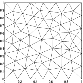
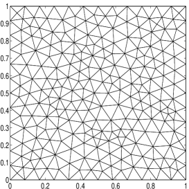
Figure 1: The coarse and fine initial meshes for the unit square (left: H=1/6 and right: H=1/12)

Figure 2 gives the corresponding numerical results for the GPE problem on the initial mesh illustrated by the left mesh in Figure 1. The corresponding numerical results for the GPE problem on the initial mesh illustrated by the right mesh in Figure 1 are shown in Figure 3.

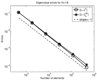
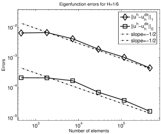
Figure 2: The errors of the cascadic multigrid algorithm for the GPE problem, where $u^{h}$ and $\lambda^{h}$ denote the eigenfunction and eigenvalue approximation by Algorithm 3.2, and $u_{h}^{\rm dir}$ and $\lambda_{h}^{\rm dir}$ denote the eigenfunction and eigenvalue approximation by direct eigenvalue solving (The left figure is the eigenvalue errors and the right figure is the eigenfunction errors which both correspond to the left mesh in Figure 1)

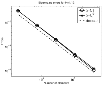
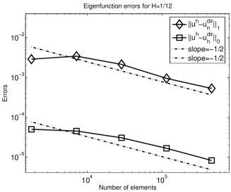
Figure 3: The errors of the cascadic multigrid algorithm for the GPE problem, where $u^{h}$ and $\lambda^{h}$ denote the eigenfunction and eigenvalue approximation by Algorithm 3.2, and $u_{h}^{\rm dir}$ and $\lambda_{h}^{\rm dir}$ denote the eigenfunction and eigenvalue approximation by direct eigenvalue solving (The left figure is the eigenvalue errors and the right figure is the eigenfunction errors which both correspond to the right mesh in Figure 1)

From Figures 2 and 3, we find the cascadic multigrid scheme can obtain the same optimal error estimates as the direct eigenvalue solving method for the eigenfunction approximations in the $H^{1}$-norm.

Remark 4.1.

Note that by (3.36) and (3.42), we do not prove the optimal convergence rate for eigenvalue error (i.e. $\big{|}\bar{\lambda}_{h_{n}}-\lambda^{h_{n}}\big{|}\leq Ch_{n}^{2}$). However, it is shown in the left of Figures 2 and 3 that $\big{|}\bar{\lambda}_{h_{n}}-\lambda^{h_{n}}\big{|}\leq Ch_{n}^{2}$.

5 Concluding remarks

In this paper, we present a type of cascadic multigrid method for GPE problem based on the combination of the cascadic multigrid for boundary value problems and the multilevel correction scheme for eigenvalue problems. The optimality of the computational efficiency has been demonstrated by theoretical analysis and numerical examples.

References

[1]
R.A. Adams.
Sobolev Spaces.
Academic Press, New York, 1975.
[2]
F.A. Bornemann and P. Deuflhard.
The cascadic multigrid method for elliptic problems.
Numer. Math., 75:135–152, 1996.
[3]
E. Cancès, R. Chakir, and Y. Maday.
Numerical analysis of nonlinear eigenvalue problems.
J. Sci. Comput., 45:90–117, 2010.
[4]
W. Hackbusch.
Multi-grid Methods and Applications.
Springer-Verlag, Berlin, 1985.
[5]
X. Han and H. Xie.