Efficient Approximation Algorithms for Computing k Disjoint Restricted Shortest Paths

Abstract

Network applications, such as multimedia streaming and video conferencing, impose growing requirements over Quality of Service (QoS), including bandwidth, delay, jitter, etc. Meanwhile, networks are expected to be load-balanced, energy-efficient, and resilient to some degree of failures. It is observed that the above requirements could be better met with multiple disjoint QoS paths than a single one. Let $G=(V,\,E)$ be a digraph with nonnegative integral cost and delay on every edge, $s,\,t\in V$ be two specified vertices, and $D\in\mathbb{Z}_{0}^{+}$ be a delay bound (or some other constraint), the $k$ Disjoint Restricted Shortest Path ($k$RSP) Problem is computing $k$ disjoint paths between $s$ and $t$ with total cost minimized and total delay bounded by $D$. Few efficient algorithms have been developed because of the hardness of the problem.

In this paper, we propose efficient algorithms with provable performance guarantees for the $k$RSP problem. We first present a pseudo-polynomial-time approximation algorithm with a bifactor approximation ratio of $(1,\,2)$, then improve the algorithm to polynomial time with a bifactor ratio of $(1+\epsilon,\,2+\epsilon)$ for any fixed $\epsilon>0$, which is better than the current best approximation ratio $(O(1+\gamma),\,O(1+\frac{1}{\gamma})\})$ for any fixed $\gamma>0$ [18]. To the best of our knowledge, this is the first constant-factor algorithm that almost strictly obeys the constraint for the $k$RSP problem.

1 Introduction

1.1 Background

The disjoint quality of service (QoS) path problem is a generalization of the shortest QoS path problem and has broad applications in networking, data transmission, etc. In data networks, many applications, such as video streaming, video conferencing, and on-demand video delivery, have several QoS requirements, which require the routing between source and destination nodes to simultaneously satisfy several QoS constraints, such as bandwidth and delay. In those applications, a single link might not provide adequate bandwidth, and multiple disjoint QoS paths are often necessary. Given cost and delay as QoS constraints, the $k$ disjoint QoS path problem can be defined as follows.

Definition 1

(The $k$ disjoint QoS path problem) Given a digraph $G=(V,\,E)$, a pair of distinct vertices $s,\,t\in V$, a cost function $c:\,E\rightarrow\mathbb{Z}_{0}^{+}$, a delay function $d:\,E\rightarrow\mathbb{Z}_{0}^{+}$, and a given delay bound $D\in\mathbb{Z}_{0}^{+}$, the $k$ disjoint QoS path problem is to compute $k$ disjoint $st$-paths $P_{1},\dots,P_{k}$, i.e., $E(P_{i})\cap E(P_{j})=\emptyset$ for every $i\neq j\in\{1,\,\dots,\,k\}$, such that $d(P_{i})\leq D$ for each $i=1,\dots,k$, and the total cost of the $k$ disjoint paths is minimized.

This problem is NP-hard even when all edges of $G$ has a cost of zero [16]. The hardness result indicates that it is impossible to develop exact or polynomial-time approximation algorithms that strictly obey the delay constraint for the $k$ disjoint QoS paths problem unless P=NP. An alternative method is to compute $k$ disjoint paths with total cost minimized and a total delay bounded by $D$ (equal to $kD$ in Definition 1), and then route the packages via the $k$ paths according to their urgency priority, i.e., routing urgent packages via paths of low delay whilst deferrable ones via paths of high delay. Then, the $k$ disjoint Restricted Shortest Path ($k$RSP) problem arises as in the following:

Definition 2

(The $k$ disjoint Restricted Shortest Path problem, $k$RSP) Given a digraph $G=(V,\,E)$, a pair of distinct vertices $s,\,t\in V$, a cost function $c:\,E\rightarrow\mathbb{Z}_{0}^{+}$, a delay function $d:\,E\rightarrow\mathbb{Z}_{0}^{+}$, and a delay bound $D\in\mathbb{Z}_{0}^{+}$, the $k$ (edge) disjoint Restricted Shortest Paths (kRSP) problem is to calculate $k$ disjoint $st$-paths $P_{1},\,\dots,\,P_{k}$, such that $E(P_{i})\cap E(P_{j})=\emptyset$ for any $i\neq j\in\{1,\,\dots,\,k\}$, $\underset{i=1,\dots,k}{\sum}d(P_{i})\leq D$, and the cost of the $k$ paths is minimized.

Previous works on the $k$RSP problem are mainly bifactor approximation algorithms. An algorithm ${\cal A}$ is a bifactor $\left(\alpha,\,\beta\right)$-approximation algorithm for the $k$RSP problem if and only if for every instance of $k$RSP, ${\cal A}$ runs in polynomial time and outputs $k$ disjoint $st$-paths, and the total delay and the total cost of the computed $k$ disjoint paths are bounded by $\alpha D$ and $\beta C_{OPT}$, respectively, where $C_{OPT}$ is the cost of an optimal solution to $k$RSP, $\alpha$ and $\beta$ are positive constants. Note that a single factor $\beta$-approximation is identical to a bifactor $\left(1,\,\beta\right)$-approximation, and we will use them interchangeably in the rest of the paper.

The $k$RSP problem is a fundamental problem in multipath routing that has a variety of benefits including fault tolerance, increased bandwidth, load balance and etc. Although multipath routing is not widely deployed in practice because of the difficulty of developing efficient algorithms, research interest focus on multipath routing is growing. The reason is the development of software defined networking (SDN), which seems a wonderful place to deploy multipath routing. Controllers therein have global information of the network and stronger computational ability, which make it possible to deploy some complicated routing algorithm into the network. Our results show that $k$RSP admits efficient approximation algorithm theoretically. This may help to boost the development of multipath routing in SDN.

$k$RSP has theoretical values beyond multipath routing. It is an interesting bicriteria optimization problem, because the shortest path problem is a fundamental problem in the area of combinatorial optimization. In addition, our method on $k$RSP might be applied to other related problems.

1.2 Related Work

In general, $k$RSP is a budgeted optimization problem: given the maximum delay constraint, find $k$ disjoint paths of minimum cost, which has been well-investigated recently. Efficient algorithms have been developed for budgeted matching and budgeted matroid intersection [2, 6]. However, those methods can not be adopted to solve $k$RSP because $k$RSP cannot be modeled as matching or matroid intersection. Another budgeted network design problem, the shallow-light Steiner tree (SLST) problem, is attracting lots of research interest. SLST is to compute a minimum cost tree spanning a set of given terminals, such that the cost of the computed tree is minimized and the delay from a specified terminal to every other terminal is not larger than $D$. This problem can not be approximated better than factor $(1,\,\gamma\log^{2}n)$ for some fixed $\gamma>0$ unless $NP\subseteq DTIME(n^{\log\log n})$ [19]. Further, although the inapproximability result doesn’t exclude the existence of polylogarithmic factor approximation algorithms for SLST, to the best of our knowledge, no such algorithms within polynomial time complexity have been developed. The algorithm with the best ratio is a long standing result by Charikar et al, which is a polylogarithmic approximation algorithm that runs in quasi-polynomial time, i.e., a factor-$O(\log^{2}t)$ approximation algorithm within time complexity $n^{O(\log t)}$[5]. Due to the difficulty in designing single factor approximation algorithms, bifactor approximation algorithms have been investigated. Hajiaghayi et al presented an $(O(\log^{2}t),\,O(\log^{4}t))$-approximation algorithm that runs in polynomial time [13]. Besides, Kapoor and Sarwat designed an approximation algorithm with bifactor $(O(\frac{p\log t}{\log p}),O(\frac{\log t}{\log p}))$, where $p$ is an input parameter [14]. Their algorithm is an approximation algorithm that improves the cost of the tree, and is with bifactor $(O(t),\,O(1))$ when $p=t$ [14]. It is even more interesting that, for the special case $S=V$, Charikar et al’s ratio of $O(\log^{2}n)$ [5] (with quasi-polynomial time complexity $n^{O(\log n)}$) is still the best single factor ratio. In addition, the existing bifactor approximations for SLST are also the known currently best approximations for the special case.

Special cases of $k$RSP have also been studied. When the delay constraint is removed, this problem is reduced to the min-sum disjoint path problem of calculating $k$ disjoint paths with the total cost minimized. This problem is known polynomially solvable [20]. Moreover, when $k=1$, the problem reduces to the single restricted shortest path (RSP) problem, which is known as a basic QoS routing problem [7] and admits fully polynomial-time approximation scheme (FPTAS) [7, 17]. The (single) QoS path problem with multiple constraints is still attracting considerable research interests. Xue et al. recently proposed a ($1+\epsilon$)-approximation algorithm [23]. When the delay constraint is on each single path, and the cost on every edge is zero, the $k$RSP problem reduces to the length-bounded disjoint path problem of finding two disjoint paths with the length of each path constrained by a given bound. This problem is a variant of the Min-Max problem, which is to find two disjoint paths with the length of the longer one minimized. Both problems are known to be NP-complete [16] with the best possible approximation ratio of 2 in digraphs [16], which can be achieved by applying the algorithm for the min-sum problem in [20, 21]. In contrast, the min-min problem of finding two disjoint paths with the length of the shorter path minimized is also NP-complete but doesn’t admit $k$-approximation for any $k\geq 1$ [3, 11, 22]. The problem remains NP-complete and admits no polynomial-time approximation scheme in planar digraphs [10].

A closely related problem, the $k$ disjoint bi-constrained path problem ($k$BCP), targets $k$ disjoint $st$-paths that satisfy the given cost constraint $\underset{i=1,\dots,k}{\sum}c(P_{i})\leq C$ and the given delay constraint $\underset{i=1,\dots,k}{\sum}d(P_{i})\leq D$. For the $k$BCP problem, approximation algorithms with a bifactor approximation ratio of $(1+\beta,\,\max\{2,\,1+\ln\frac{1}{\beta})$ or a single factor ratio of $O(\ln n)$ (i.e. bifactor approximation ratio $(1,\,O(\ln n))$) have been developed for general $k$ in [12], where $\beta>0$ is any fixed positive real number. Apparently, $k$BCP is a weaker version of $k$RSP, and hence all approximations of $k$RSP can be adopted to solve $k$BCP, but not the other way around.

The $k$RSP problem itself has attracted considerable research interest of a number of computer scientists. [4] and [18] have achieved bifactor ratios of $(1+\frac{1}{r},\,r(1+\frac{2(\log r+1)}{r})(1+\epsilon))$ and $(1+\frac{1}{r},\,1+r)$ for $k=2$, respectively. Based on LP-rounding technology, an approximation with bifactor ratio $(2,\,2)$ has been developed in [9]. To the best of our knowledge, however, no algorithm has achieved a constant single factor approximation ratio for decades. Our algorithm is the first one showing that $k$RSP admits a almost constant single factor approximation ratio theoretically.

1.3 Our Results

The main results of this paper are summarized in this section with proofs detailed in latter sections.

Lemma 3

The $k$RSP problem admits an approximation algorithm with an approximation ratio of $(1,\,2)$ and runtime $O((\sum c(e))^{2}\sum d(e)(n^{4.5}C_{OPT}^{4.5}DL))$, where $C$ is the cost of an optimal solution and $L$ is the maximum length of the input.

We note that the algorithm is with pseudo-polynomial time complexity, because the above formula of the time complexity involves $C_{OPT}$, $D$, and edge costs and edge delays of the graph. However, by applying the traditional technique for polynomial time approximation scheme design as in [7], we can immediately obtain a polynomial time algorithm with bifactor approximation ratio ($1+\epsilon_{1},\,2+\epsilon_{2}$). Below is the main idea of the technique: For any constant $\epsilon_{1},\,\epsilon_{2}>0$, set the delay and cost of every edge $e$ to $\left\lfloor\frac{d(e)}{\frac{\epsilon_{1}D}{n}}\right\rfloor$ and $\left\lfloor\frac{c(e)}{\frac{\epsilon_{2}C_{OPT}}{n}}\right\rfloor$, respectively. Then the time complexity of the algorithm becomes polynomial time, since

$$O((\sum c(e))^{2}\sum d(e)(n^{4.5}C_{OPT}^{4.5}DL))$$

$$\leq O(\sum^{2}\left\lfloor\frac{c(e)}{\frac{\epsilon_{2}C_{OPT}}{n}}\right\rfloor\sum\left\lfloor\frac{d(e)}{\frac{\epsilon_{1}D}{n}}\right\rfloor(n^{4.5}(\frac{n}{\epsilon_{2}})^{4.5}\frac{n}{\epsilon_{1}}L))$$

$$\leq O(m^{3}n^{12}\frac{1}{\epsilon_{1}^{2}\epsilon_{2}^{6.5}})$$

.

Theorem 4

For any constants $\epsilon_{1},\,\epsilon_{2}>0$, the $k$RSP problem admits a polynomial time algorithm with an approximation ratio $(1+\epsilon_{1},\,2+\epsilon_{2})$.

The time complexity of the algorithm can be analyzed better. Anyhow, to the best of our knowledge, this is the first constant factor approximation algorithm for the $k$RSP problem that runs in polynomial time, and almost strictly obeys the delay constraint. Note that we can set $\epsilon_{1}=\epsilon_{2}=\epsilon$, and the approximation ratio will be $(1+\epsilon,\,2+\epsilon)$, as we claimed in the abstract.

Our pseudo polynomial time approximation algorithm of Lemma 3 mainly consists of two phases. The first phase is to compute a not-too-bad solution for the $k$RSP problem by a simple LP-rounding algorithm as in [9], whose performance guarantee has been shown as in the following:

Lemma 5

The $k$RSP problem admits an algorithm, such that for any of its output solutions, there exists a real number $0\leq\alpha\leq 2$ such that the delay-sum and the cost-sum of the solution are bounded by $\alpha D$ and $(2-\alpha)*C_{OPT}$, respectively.

Note that $\alpha$ differs for different instances, i.e., the algorithm might return a solution with cost $2C_{OPT}$ and delay $0$ for some instances, whilst a solution with cost 0 and delay $2D$ for other instances. So the bifactor approximation ratio for the algorithm is actually $(2,2)$. The second phase of our algorithm, as the main task of this paper, is to improve the approximation ratio $(2,\,2)$ to $(1+\epsilon,\,2+\epsilon)$ in pseudo polynomial time.

The main techniques involved in the second phase include the cycle cancellation method, LP-rounding, and some graph transformations techniques. We would like to remark here that the cycle cancellation method is a classic framework that has been used to solve numerous problems related to shortest path, minimum cost flow and etc [1, 12, 18]. However, to the best of our knowledge, in previous works the cycles used are computed in a graph which allows either negative-cost edges or negative-delay edges, but not both. Because no polynomial algorithm is known for computing a best cycle for cycle cancellation in a graph allowing both negative cost and delay. This paper not only gives an approximation algorithm for the $k$RSP problem, but also enhances the cycle cancellation method by giving a novel algorithm of computing bicameral cycle, which is a good-enough cycle for cycle cancellation in a graph where both negative-cost edges and negative-delay edges are allowed (The formal definition of bicameral cycles will be given later). That is, our algorithm can hopefully improve the approximation ratios of other bicriteria optimization problems (or namely budgeted optimization problems) in which the cycle cancellation method can be suitably applied.

The remainder of the paper is organized as below: Section 2 introduces cycle cancellation, Section 3 gives the definition of bicameral cycles, and then shows that using bicameral cycles in cycle cancellation can result in a desired approximation ratio $(1+\epsilon_{1},\,2+\epsilon_{2})$. This is the first tricky task of this paper. Section 4 gives the algorithm that actually computes a bicameral cycle in polynomial time, which is the most tricky task of this paper. Section 5 concludes this paper.

2 The cycle cancellation method for $k$RSP

This section will give the key idea of an improved approximation for $k$RSP based on the cycle cancellation method. We shall first state our version of the cycle cancellation method (and point out the difference comparing to previous versions), then give the improved algorithm that is an enhancement to the cycle cancellation technique.

2.1 The Cycle Cancellation Method

We would like to start from some definitions and notations. Let $E_{1}$ and $E_{2}$ be two set of edges. Then $E_{1}\oplus E_{2}$ denotes the edge set $E_{1}\cup E_{2}\setminus\{e(u,\,v)|\{e(u,\,v),\,e(v,\,u)\}\subseteq E_{1}\cup E_{2}\}$, i.e., $E_{1}\cup E_{2}$ except pairs of parallel edges in opposite direction therein. Let $P$ be a $st$-path and $\overline{P}=\{e^{\prime}(v,u)|e(u,v)\in P\}$, i.e., $\overline{P}$ is $P$ but with the direction of each edge reversed. Moreover, the cost and delay of the edges of $\overline{P}$ are negatived, i.e., $c(e^{\prime}(v,\,u))=-c(e(u,\,v))$ and $d(e^{\prime}(v,\,u))=-d(e(u,\,v))$ for every edge $e^{\prime}(v,\,u)\in\overline{P}$.

Definition 6

(Residual graph) A residual graph $\widetilde{G}=G_{res}(P_{1},\,\dots,\,P_{k})$, with respect to $G$ and $P_{1},\,\dots,\,P_{k}\subset G$, is graph $G\cup(\underset{i=1,\,\dots,\,k}{\cup}E(\overline{P_{i}}))\setminus\underset{i=1,\,\dots,\,k}{\cup}E(P_{i})$, i.e., graph $G$ with the direction of edges of $P_{1},\,\dots,\,P_{k}$ reversed, and their cost and delay negatived.

For notation briefness, we use $\widetilde{G}$ instead of $G_{res}(P_{1},\,\dots,\,P_{k})$ while no confusion arises. In literature [12] and [18], the authors also employed the cycle cancellation method. However, in their constructed residual graph, the cost of reversed edge $e^{\prime}(v,u)$ is sat $c(e^{\prime}(v,u))=0$ instead of $c(e^{\prime}(v,u))=-c(e(u,v))$, such that the edges in their residual graphs are with nonnegative cost. Then, the minimum-mean-cycle algorithm can be applied therein, and hence a best cycle for cycle cancellation, i.e., $O$ with $\frac{d(O)}{c(O)}$ minimized, can be computed in polynomial time [15]. Note that for a more complicated residual graph as in Definition 6, the method above can not be applied to compute a best cycle any longer.

The cycle cancellation method is based on the following proposition which can be derived from the flow theory:

Proposition 7

Let $P_{1},\,\dots,\,P_{k}$ be $k$ disjoint $st$-paths in $G$ and $O_{1},\,\dots,\,O_{h}$ be a set of edge-disjoint cycles in residual graph $\widetilde{G}$. Then $\{P_{1},\,\dots,\,P_{k}\}\oplus\{O_{1},\,\dots,\,O_{h}\}$ contains $k$ disjoint $st$-paths in $G$.

Proof 2.1.

Following the flow theory, we need only to show that $\{P_{1},\,\dots,\,P_{k}\}\oplus\{O_{1},\,\dots,\,O_{h}\}$contains an integral $st$-flow of value $k$ and the flow is a valid flow in $G$.

Firstly, $\{P_{1},\,\dots,\,P_{k}\}\oplus\{O_{1},\,\dots,\,O_{h}\}$ contains an integral flow of value $k$ that goes from $s$ to $t$. That is because $s$ and $t$ are respectively with degree $k$ and $-k$ in $P_{1}\cup\,\dots\,\cup P_{k}$ whilst every vertex are with degree 0 in $O_{1},\,\dots,\,O_{h}$. So $s$ and $t$ are respectively with degree $k$ and $-k$ while every other vertex is with degree 0 in $\{P_{1},\,\dots,\,P_{k}\}\oplus\{O_{1},\,\dots,\,O_{h}\}$.

Secondly, $\{P_{1},\,\dots,\,P_{k}\}\oplus\{O_{1},\,\dots,\,O_{h}\}$ is a valid flow in $G$. On one hand, every edge appears at most once in the flow of$\{P_{1},\,\dots,\,P_{k}\}\oplus\{O_{1},\,\dots,\,O_{h}\}$ (i.e. satisfies the capacity constraint). That is because every edge appears at most once in $\{P_{1},\,\dots,\,P_{k}\}\oplus\{O_{1},\,\dots,\,O_{h}\}$, since$\{P_{1},\,\dots,\,P_{k}\}$ and $\{O_{1},\,\dots,\,O_{h}\}$ shares no common edges, and the paths of $\{P_{1},\,\dots,\,P_{k}\}$ are mutually edge-disjoint and so are the cycles of $\{O_{1},\,\dots,\,O_{h}\}$. On the other hand, $\{P_{1},\,\dots,\,P_{k}\}\oplus\{O_{1},\,\dots,\,O_{h}\}$ contains only edges of $G$, since every edge of $\{O_{1},\,\dots,\,O_{h}\}\setminus G$ has a parallel opposite counterpart in $\{P_{1},\,\dots,\,P_{k}\}$.

Intuitively, $\{P_{1},\,\dots,\,P_{k}\}\oplus\{O_{1},\,\dots,\,O_{h}\}$ is to replace the edges of $P_{1},\,\dots,\,P_{k}$, which have parallel opposite counterpart in $\{O_{1},\,\dots,\,O_{h}\}$, by the edges of $\{O_{1},\,\dots,\,O_{h}\}\setminus\{\overline{P}_{1},\,$ $\dots,\,\overline{P_{k}}\}$. Such an edge replacement with cycles is called cycle cancellation.

2.2 Cycle Cancellation with Bicameral Cycles for $k$RSP

This subsection shall apply the cycle cancellation method to improve a solution of the $k$RSP problem. Let $P_{1},\,\dots,\,P_{k}$ be a solution resulting from the first phase with large delay, say $\sum_{i=1}^{k}d(P_{i})>D$. According to Proposition 7, if we could find a set of edge-disjoint negative delay cycles $O_{1},\,\dots,\,O_{h}$, then we could decrease the delay of the solution to $k$RSP by using $\{P_{1},\,\dots,\,P_{k}\}\oplus\{O_{1},\,\dots,\,O_{h}\}$ as the $k$ disjoint paths. Naturally, a question arises:

Does there always exist cycles with negative delay in $\widetilde{G}$ when $\sum_{i=1}^{k}d(P_{i})>D$ holds?

To answer this question, the following proposition is necessary:

Proposition 8.

Let $P_{1}^{*},\,\dots,\,P_{k}^{*}$ be a minimum cost solution to the $k$RSP problem that satisfies the delay constraint, and $P_{1},\,\dots,\,P_{k}$ be $k$ disjoint $st$-paths. Then $\{P_{1}^{*},\,\dots,\,P_{k}^{*}\}\oplus\{\overline{P_{1}},\,\dots,\,\overline{P_{k}}\}$ is exactly a set of edge-disjoint cycles.

The key idea to prove the proposition is that: Every vertex in graph $\{P_{1}^{*},\,\dots,\,P_{k}^{*}\}\oplus\{\overline{P_{1}},\,\dots,\,\overline{P_{k}}\}$ is with degree 0, so $\{P_{1}^{*},\,\dots,\,P_{k}^{*}\}\oplus\{\overline{P_{1}},\,\dots,\,\overline{P_{k}}\}$ is composed by exactly a set of cycles. We note that a generalized version (for network flow) of Proposition 8 has appear in [1], so we omit the detailed proof here. Let $\{O_{1},\dots,O_{h}\}$ be the set of cycles of $\{P_{1}^{*},\,\dots,\,P_{k}^{*}\}\oplus\{\overline{P_{1}},\,\dots,\,\overline{P_{k}}\}$. Note that $\sum_{i=1}^{k}d(P_{i})>\sum_{i=1}^{k}d(P_{i}^{*})$, so $\sum_{i=1}^{h}d(O_{i})=\sum_{i=1}^{k}d(P_{i}^{*})-\sum_{i=1}^{k}d(P_{i})<0$ holds, and hence at least one cycle of $\{O_{1},\dots,O_{h}\}$ is with negative delay. Hence, the previous question has a positive answer, formally as below:

Lemma 9.

If $\sum_{i=1}^{k}d(P_{i})>D$, then there exists at least one cycle with negative delay in $\widetilde{G}$.

From Proposition 7 and Proposition 8, an idea for the improved algorithm is to find the set of cycles $\{O_{1},\dots,O_{h}\}$ and use them to improve the $k$ disjoint paths $P_{1},\,\dots,\,P_{k}$ to an optimal solution $P_{1}^{*},\,\dots,\,P_{k}^{*}$. However, it is hard to identify all the cycles $\{O_{1},\,\dots,\,O_{h}\}$ exactly. So the key idea of the improved algorithm is generally a greedy approach, which repeats computing a “best” cycle (i.e. cycle $O$ with optimum $\frac{d(O)}{c(O)}$), and using it to improve the current $k$ disjoint paths towards an optimal solution, until a desired solution is obtained. However, a “best” cycle is probably NP-hard to compute. So our algorithm use a bicameral cycle instead. Let $P_{1},\,\dots,\,P_{k}$ be the current solution to the $k$RSP problem. Then the main steps of our algorithm roughly proceeds as below:

While $\sum_{i=1}^{k}d(P_{i})>D$ do

  Compute a bicameral cycle $O$;

  Set $\{P_{1},\,\dots,\,P_{k}\}\leftarrow\{P_{1},\,\dots,\,P_{k}\}\oplus O$.

3 Proof of Lemma 3

This section will first give the formal definition of bicameral cycles as well as the formal layout of our algorithm, then show that, by using the defined bicameral cycles, our algorithm can output a solution with a bifactor ratio $(1,\,2)$, and terminate in pseudo polynomial time.

3.1 The Improved Algorithm

Let $P_{1},\,\dots,\,P_{k}$ be a feasible solution to $k$RSP. W.l.o.g., assume $\sum_{i=1}^{k}d(P_{i})>D$. Let $\Delta D=D-\sum_{i=1}^{k}d(P_{i})$ and $\Delta C=C_{OPT}-\sum_{i=1}^{k}c(P_{i})$, where $C_{OPT}$ is the cost of an optimal solution to $k$RSP. Let $O$ be a cycle in the residual graph wrt $P_{1},\,\dots,\,P_{k}$. Then because the meaning of $\frac{d(O)}{c(O)}$ depends on positive or negative $d(O)$ (or $c(O)$). So we have three types of bicameral cycles accordingly, as in the following:

Definition 10.

(bicameral cycles)

1. If $d(O)<0$ and $c(O)\leq 0$ or $d(O)\leq 0$ and $c(O)<0$, then $O$ is a (type-0) bicameral cycle;

2. Otherwise,

   1. If $d(O)<0$ and $0<c(O)\leq C_{OPT}$, then $O$ is a (type-1) bicameral cycle iff $\frac{d(O)}{c(O)}\leq\frac{\Delta D}{\Delta C}$, where $\Delta D=D-\sum_{i=1}^{k}d(P_{i})$ and $\Delta C=\sum_{i=1}^{k}c(P_{i}^{*})-\sum_{i=1}^{k}c(P_{i})$;

   2. If $d(O)\geq 0$ and $-C_{OPT}\leq c(O)<0$, then $O$ is a (type-2) bicameral cycle iff $\frac{d(O)}{c(O)}\geq\frac{\Delta D}{\Delta C}$.

Clearly, a type-0 bicameral cycle is the first choice for our algorithm, because it can be used to decrease the delay of the $k$ disjoint paths without any cost increment according to our algorithm. Differently, using a type-1 (2) cycle $O$ for cycle cancellation will decrease delay (cost), but increase the cost (delay) of the current solution. Since computing a bicameral cycle is one of two tricky tasks of this paper, the algorithm will be deferred to Section 4. The formal layout of our algorithm is as in Algorithm 1.

Input: Graph $G$, specified vertices $s$ and $t$, a cost function $c(e)$ and a delay function $d(e)$ on edge $e$, and a delay bound $D\in\mathbb{Z}_{0}^{+}$;

Output: $\{P_{1},\dots,P_{k}\}$, the set of edges that compose $k$ disjoint $st$-paths.

1. Compute $k$ disjoint $st$-paths $P_{1},\dots,P_{k}$ by the LP-rounding algorithm as in [9];

2. While $\sum_{i=1}^{k}d(P_{i})>D$ do

   1. If there exists no bicameral cycle in $\widetilde{G}$, then return “infeasible”; /*The instance is infeasible.*/

   2. Compute a bicameral cycle $O$;

   3. $\{P_{1},\dots,P_{k}\}\leftarrow\{P_{1},\dots,P_{k}\}\oplus O$;

3. Return $\{P_{1},\dots,P_{k}\}$.

Algorithm 1 An improved algorithm for $k$RSP.

We would like to give some remarks on the definition of bicameral cycles before presenting the ratio proof. Firstly, a bicameral cycle $O$ is not a “best” cycle, it suffices only $\frac{d(O)}{c(O)}\leq\frac{\Delta D}{\Delta C}$ (type 1 bicameral cycle for example). There may be other far better cycles for cycle cancellation, but it takes too long to compute. Secondly, a type-1 bicameral cycle $O_{1}$ must satisfy an additional constraint $0<c(O_{1})\leq C_{OPT}$, and a type-1 bicameral cycle $O_{2}$ must satisfy $-C_{OPT}\leq c(O)<0$. This makes the definition of bicameral cycle more complicated, but it is essential. Since without the constraint, the ratio of the algorithm will become $(1+\alpha,\,1+\frac{1}{\alpha})$. In this case, the cost of the solution resulting from the algorithm could be very large when $\alpha$ is a small number, say $\alpha=\frac{1}{D}$ (see Figure 1 for example).

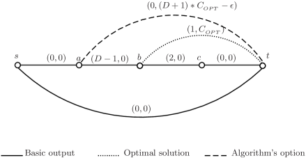
Figure 1: An example for execution of Algorithm 1 without consider the constraint on the cost: $sabct$ and $st$ is the solution resulted from the simple approximation algorithm in [17, 9]; $sat$ and $st$ would the output of the algorithm, with cost $C_{OPT}*(D+1)-\epsilon$ and delay $0$; while the optimal solution is $sabt$ and $st$, with cost $C_{OPT}$ and delay $D$.

Because of the complicated constraints on type-1 and type-2 bicameral cycles, and the fact that the residual graph defined in this paper allows both negative cost and delay on edges, previous techniques as in [9, 18, 12] are not suitable for computing a bicameral cycle. Anyhow, this paper figures out a constructive method for computing bicameral cycles, which will be shown in Section 4.

3.2 Proof of Approximation Ratio and Time Complexity

Assume that the algorithm terminates in $f$ iterations. Without loss of generality, assume that $f>1$. Let $O_{i}$ be a bicameral cycle in the $i$th iteration, and $D_{i}$ and $C_{i}$ be the delay and cost of the current solution, respectively. Let $\Delta D_{i}=D-D_{i}$, $\Delta C_{i}=C_{OPT}-C_{i}$, and $r_{i}=\frac{\Delta D_{i}}{\Delta C_{i}}$. The ratio of Algorithm 1 is as below:

Lemma 11.

If the $k$RSP problem is feasible, Algorithm 1 outputs a solution with delay strictly bounded by $D$ and cost bounded by $2C_{OPT}$.

Proof 3.1.

Algorithm 1 terminates only when the delay constraint is satisfied. Then from Lemma 9, the lemma is obviously true for the delay constraint part. For the cost part, according to the definition of bicameral cycles, the cost augmentation in the last iteration, i.e., the $f$th iteration, is at most $C_{OPT}$. Then we need only to show that $C_{f-1}\leq C_{OPT}$. Below is the detailed proof by using mathematical induction. According to Lemma 5, for the cost $C_{0}$ and delay $D_{0}$ of the first phase, there exist $0\leq\alpha\leq 2$, such that $C_{0}=\alpha C_{OPT}$ and $D_{0}=(2-\alpha)D$. Then since the algorithm didn’t terminate in the first iteration, we have $D_{0}>D$ and $C_{0}<C_{OPT}$. By induction, $C_{i}<C_{OPT}$ holds. It remains only to prove $C_{i+1}<C_{OPT}$ for the case $C_{i+1}>C_{i}$. That is, the computed bicameral cycle $O_{i}$ suffices $c(O_{i})>0$. According to the definition of type-1 bicameral cycles, we have

$$\frac{d(O_{i})}{c(O_{i})}=\frac{D_{i+1}-D_{i}}{C_{i+1}-C_{i}}\leq\frac{\Delta D_{i}}{\Delta C_{i}}=\frac{D-D_{i}}{C_{OPT}-C_{i}}.$$ (1)

Before the $f$th iteration the delay of the solution is always larger than $D$, so $D_{i+1}>D$ and $D_{i}>D$ both hold. Thus, we have:

$$0>D_{i+1}-D_{i}>D-D_{i}.$$ (2)

Combining Inequality (1) and Inequality (2) yields $C_{i+1}-C_{i}<C_{OPT}-C_{i}$, so $C_{i+1}<C_{OPT}$. This completes the proof.

The statement of this lemma is only for the case that the $k$RSP problem is feasible. When the instance for $k$RSP is infeasible, i.e., there does not exist $k$ disjoint paths satisfying the delay constraint $D$, Algorithm 1 will detect the infeasibility and return “infeasible” in Step 2(a).

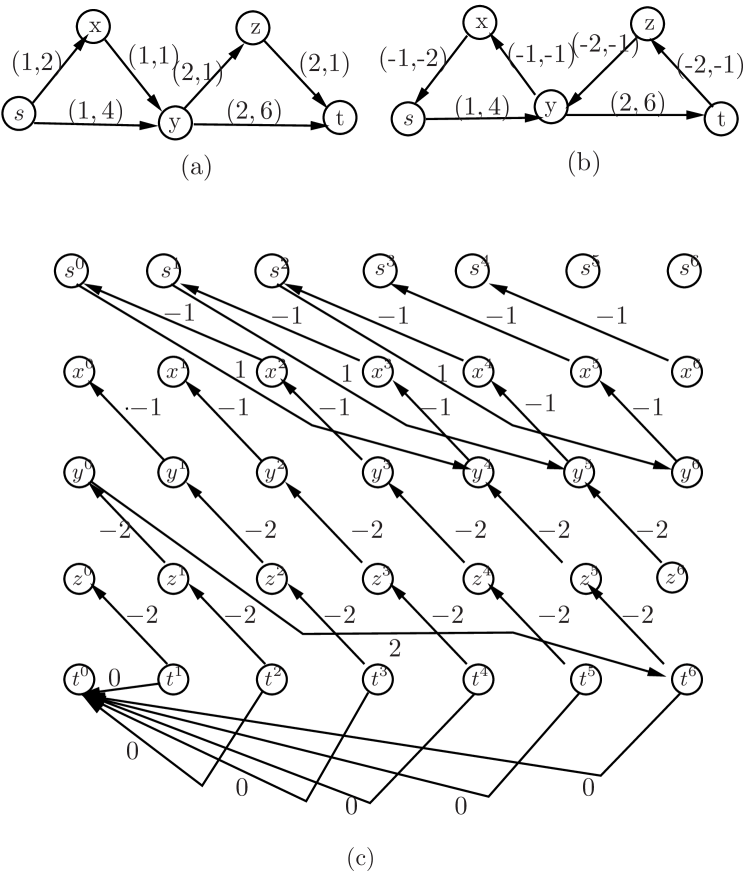
Figure 2: Construction of auxiliary graph $H$ with cost constraint $B=6$. (a) graph $G$; (b) graph $\widetilde{G}$ wrt path $sxyzt$; (c) auxiliary graph $H$.

Before presenting the time complexity analysis of Algorithm 1, we would like first to investigate some properties of bicameral cycles, as in the following lemma:

Lemma 12.

For the $i$th iteration, $i<f$, at least one of the following two cases holds:

1. $r_{i+1}=r_{i}$ and $\Delta D_{i+1}<\Delta D_{i}$ ;

2. $r_{i+1}>r_{i}$.

Proof 3.2.

Recall that $O_{i}$ is the bicameral cycle computed in the $i$th iteration. If $O_{i}$ is a type-0 bicameral cycle, then $d(O_{i})<0$ and $-C_{OPT}\leq c(O_{i})\leq 0$, or $d(O_{i})\leq 0$ and $-C_{OPT}\leq c(O_{i})<0$ hold. For these two cases of type-0 bicameral cycle, Clause 2 obviously holds. So we need only to consider type-1 and type-2 cycles, which are as below:

1. $d(O_{i})<0$ and $0<c(O_{i})<C_{OPT}$

   According Definition 10, $\frac{d(O_{i})}{c(O_{i})}\leq r_{i}$ holds. Then we have

   $$d(O_{i})\leq r_{i}\cdot c(O_{i}).$$ (3)

   After the cycle cancellation wrt $O_{i}$, $r_{i+1}=\frac{\Delta D_{i}-d(O_{i})}{\Delta C_{i}-c(O_{i})}$. Combining this inequality with Inequality (3) yields

   $$r_{i+1}\geq\frac{\Delta D_{i}-r_{i}\cdot c(O_{i})}{\Delta C_{i}-c(O_{i})}=r_{i}\cdot\frac{\Delta C_{i}-c(O_{i})}{\Delta C_{i}-c(O_{i})}=r_{i}.$$ (4)

   Since $d(O_{i})<0$, $\Delta D_{i+1}<\Delta D_{i}$ holds. So if the two sides of Inequality (4) are equal, Clause 1 holds; otherwise Clause 2 holds.

2. $-C_{OPT}<c(O_{i})<0$ and $d(O_{i})>0$

   The proof of the second case is similar to the first case. $O_{i}$ is with maximum $\frac{d(O_{i})}{c(O_{i})}$ according to Definition 10, so $\frac{d(O_{i})}{c(O_{i})}>r_{i}$ holds, and hence

$$d(O_{i})<r_{i}\cdot c(O_{i}).$$ (5)

Then combining the above inequality with $r_{i+1}=\frac{\Delta D_{i}-d(O_{i})}{\Delta C_{i}-c(O_{i})}$, we have

$$r_{i+1}>\frac{\Delta D_{i}-r_{i}\cdot c(O_{i})}{\Delta C_{i}-c(O_{i})}=r_{i}\frac{\Delta C_{i}-c(O_{i})}{\Delta C_{i}-c(O_{i})}=r_{i}.$$

Therefore, Clause 2 always holds for case 2. This completes the proof.

Let $t_{bc}$ be the time of computing a bicameral cycle. We now consider the time complexity of the algorithm. The key observation is that $r_{i}$ is an arbitrary number. In fact, there are at most $\sum c(e)*\sum d(e)$ different values for $r$. That is because for the formula $r_{i}=\frac{\Delta D_{i}}{\Delta C_{i}}$, the value of $\Delta D_{i}$ must be an integer between 0 and $-\sum d(e)$, and so is $\Delta C_{i}$. Then according to Lemma 12, the algorithm computes at most $\sum c(e)*\sum d(e)$ bicameral cycles to decrease the value of $r_{i}$. On the other hand, the algorithm computes at most $|D|*\sum c(e)*\sum d(e)$ bicameral cycles to decrease the delay sum of the $k$ disjoint paths (Note that $\Delta D_{i}>\Delta D_{i+1}$ may hold). Therefore, we have the following lemma:

Lemma 13.

The time complexity of our algorithm is $O(|D|*\sum c(e)*\sum d(e)*t_{bc})$.

The time complexity of our algorithm can be analyzed better. However, we omit the detailed and sophisticated analysis, because the length limit, and the focus of this paper should be on the approximation ratio.

4 Computing Bicameral Cycle $O_{i}$

This section will show how to compute a bicameral cycle $O_{i}$. This task is not easy, because almost every task involving bicriteria negative cycle is NP-hard. The key idea of our algorithm is to construct two auxiliary graphs $H_{v}^{+}(B)$ and $H_{v}^{-}(B)$, such that every cycle containing $v$ with total cost between $0$ and $B$ in $\widetilde{G}$ is corresponding to a cycle in $H_{v}^{+}(B)$ while every cycle containing $v$ with cost between $-B$ and $0$ corresponds to a cycle in $H_{v}^{-}(B)$, where $B$ is a given bound on cost and $v$ is a vertex of $\widetilde{G}$. Then by computing the cycles in $H_{v}^{+}(B)$ and $H_{v}^{-}(B)$ for every $v\in\widetilde{G}$ and every necessary $B$, we could find in $\widetilde{G}$ bicameral cycles if there exists any. The construction of auxiliary graph will be given in Subsection 4.1 and the other parts of the algorithm shall be given in Subsection 4.2.

4.1 Construction of Auxiliary Graph $H_{v}(B)$

The algorithm of constructing the auxiliary graph $H_{v}^{+}(B)$ and $H_{v}^{-}(B)$ is inspired by the method of modeling a shallow-light spanning tree path subject to multiple constraints [8]. The full layout of the construction $H_{v}^{+}(B)$ is as shown in Algorithm 2 (An example of such a construction is as depicted in Figure 2).

Input: Residual graph $\widetilde{G}$ with edge cost $c:\,e\rightarrow\mathbb{Z}_{0}^{+}$ and edge delay $d:\,e\rightarrow\mathbb{Z}_{0}^{+}$, a specified vertex $v\in V$, a given cost constraint $B\in\mathbb{Z}^{+}$;

Output: Auxiliary graph $H_{v}^{+}(B)$.

1. For every vertex $v_{l}$ of $V$ do

   Add $B+1$ vertices $v_{l}^{0},\dots,v_{l}^{B}$ to $H_{v}^{+}(B)$ ;

2. For every edge $e=\left\langle v_{j},v_{l}\right\rangle\in E$ do

   1. if $c(e)\geq 0$, add to $H_{v}^{+}(B)$ the edges $\left\langle v_{j}^{0},\,v_{l}^{c(e)}\right\rangle,\,\dots,\left\langle v_{j}^{B-c(e)},\,v_{l}^{B}\right\rangle$, each of which is with delay $d(e)$;

   2. if $c(e)<0$, add to $H_{v}^{+}(B)$ the edges $\left\langle v_{j}^{B},\,v_{l}^{B-|c(e)|}\right\rangle,\,\dots,\left\langle v_{j}^{|c(e)|},\,v_{l}^{0}\right\rangle$, each of which is with delay $d(e)$.

3. For each vertex $v^{i}$ of $H_{v}^{+}(B)$ that corresponding to the specified vertex $v\in G$ do

   Add edge $e(v^{i},\,v^{0})$ to $H_{v}^{+}(B)$ with delay zero. /* To construct $H_{v}^{-}(B)$ is to add edge $e(v^{i},\,v^{B})$. */

Algorithm 2 Construction of auxiliary graph $H_{v}^{+}(B)$.

4.2 Computation of Bicameral Cycle $O_{i}$

This subsection shall show how to use LP-rounding method to compute cycles in $H_{v}^{+}(B)$ and $H_{v}^{-}(B)$, and obtain a bicameral cycle in $\widetilde{G}$. We start from the following linear programming formula:

$$\min\sum_{e\in H}c(e)x(e)$$ (6)

subject to

$$\sum_{e\in\delta^{+}(v)}x_{e}-\sum_{e\in\delta^{-}(v)}x_{e}=\begin{array}[]{cc}0&\forall v\in V(H_{v}^{+}(B)\,or\,H_{v}^{-}(B))\end{array}$$

$$\sum_{e\in H}d(e)x(e)\leq\Delta D$$

Unlike other linear programming formula for shortest paths, spanning trees, or Steiner trees, $0\leq x(e)\leq 1$ is not necessary for our formula, because our goal is only to compute a bicameral cycle. Below we shall discuss $H_{v}^{+}(B)$ only, since the case for $H_{v}^{-}(B)$ is similar.

Lemma 14.

A solution to LP (6) exactly corresponds to a set of cycles with cost between $B$ and $-B$ in residual graph $\widetilde{G}$.

A solution to LP (6) is apparently corresponding to a set of fractional cycles of $H_{v}^{+}(B)$ (or $H_{v}^{-}(B)$). So we need only to show that a cycle in $H_{v}^{+}(B)$ corresponds to a set of cycles in $\widetilde{G}$. In fact, according to the construction of $H_{v}^{+}(B)$ , we have the following lemma, from which the correctness of Lemma 14 can be immediately obtained.

Lemma 15.

A cycle in $H_{v}^{+}(B)$ corresponds to a set of cycles in $\widetilde{G}$, each of which is with cost between $B$ and $-B$. Conversely, a cycle in $\widetilde{G}$, containing $v$ and with cost between $0$ and $B$, corresponds to a cycle in $H_{v}^{+}(B)$.

Proof 4.1.

Assume that $O$ is a cycle in $H_{v}^{+}(B)$. According to the rules of adding the edges of $H_{v}^{+}(B)$, every edge in $H_{v}^{+}(B)$ either corresponds to an edge in $\widetilde{G}$ or is between duplications of an identical vertex of $\widetilde{G}$. So $O$ corresponds to a closed walk in $\widetilde{G}$, and hence it corresponds to a set of cycles of $\widetilde{G}$. The cost bound of the set of cycles follows from the construction of $H_{v}^{+}(B)$ similarly.

Conversely, let $O^{\prime}$ be a cycle in $\widetilde{G}$, with cost between $0$ and $B$, i.e., $0\leq c(O^{\prime})\leq B$. Start from $v^{0}\in H_{v}^{+}(B)$, a vertex corresponding to $v\in O^{\prime}$, according to the edges on $O^{\prime}$, we can find a path from $v^{0}$ to $v^{c(O^{\prime})}$, since $c(O^{\prime})\leq B$. The path plus the edge $e(v^{c(O^{\prime})},v^{0})$ exactly compose a cycle in $H_{v}^{+}(B)$.

Theorem 16.

Let cycles $O_{1},\dots,O_{z}$ be the cycles in $\widetilde{G}$ corresponding to $\chi(v,B^{*})$ for every $v\in\widetilde{G}$, where $B^{*}=\sum_{i=1}^{k}c(P_{i}^{*})$ and $P_{1}^{*},\dots,P_{k}^{*}$ is an optimal solution to the $k$RSP problem. Then there must be a bicameral cycle in $O_{1},\dots,O_{z}$ if the $k$RSP problem is feasible.

Proof 4.2.

If there exist $c(O_{i})\leq 0$ and $d(O_{i})<0$, or $d(O_{i})\leq 0$ and $c(O_{i})<0$, then $O_{i}$ is type-0 bicameral cycle. So without loss of generality, we can assume that either $c(O_{i})\geq 0$ or $d(O_{i})\geq 0$ holds. Let $\chi^{+}(v,\,B^{*})$ be an optimal solution to LP (6) against $H_{v}^{+}(B)$.

Let $P_{1},\dots,P_{k}$ be the current solution against $k$RSP. Let $\{O_{1}^{*},\dots,O_{h}^{*}\}=\{P_{1}^{*},\dots,P_{k}^{*}\}\oplus\{\overline{P_{1}},\dots,\overline{P_{k}}\}$. Then apparently

$$-\sum_{i=1}^{k}c(P_{i}^{*})\leq-\sum_{i=1}^{k}c(P_{i})\leq c(O_{i}^{*})\leq\sum_{i=1}^{k}c(P_{i}^{*}).$$

That is, cycle $O_{i}^{*}$ with $d(O_{i}^{*})<0$ and $c(O_{i}^{*})>0$ can find its corresponding cycle in $\cup_{v\in\widetilde{G}}H_{v}^{+}(B^{*})$. Without loss of generality assume that $O_{i}^{*}$ with minimum $\frac{d(O_{i}^{*})}{c(O_{i}^{*})}$ among all other cycles of $\{O_{1}^{*},\dots,O_{h}^{*}\}$ with negative delay, and its corresponding cycle is in $H_{v_{j}}(B^{*})$. Then we have $\frac{d(\chi(v_{j},B^{*}))}{c(\chi(v_{j},B^{*}))}\leq\frac{d(O_{i}^{*})}{c(O_{i}^{*})}$. So in the set of cycles of $\widetilde{G}$ that corresponding to $\chi^{+}(v,B^{*})$, there must exist a cycle $O_{1}$ with $\frac{d(O_{1})}{c(O_{1})}\leq\frac{d(O_{i}^{*})}{c(O_{i}^{*})}$ and $d(O_{1})<0$, or $\frac{d(O_{2})}{c(O_{2})}\geq\frac{d(O_{i}^{*})}{c(O_{i}^{*})}$ and $c(O_{2})<0$. The case for $O_{i}^{*}$ with $d(O_{i}^{*})\geq 0$, $c(O_{i}^{*})<0$ and maximum $\frac{d(O_{i}^{*})}{c(O_{i}^{*})}$ is similar in $\cup_{v\in\widetilde{G}}H_{v}^{-}(B^{*})$, and hence we can find $O^{\prime}_{1}$ and $O^{\prime}_{2}$ accordingly. Then from the definition of bicameral cycle, at least one cycle of $\{O_{1},O^{\prime}_{1},O_{2},O^{\prime}_{2}\}$ is a bicameral cycle. This completes the proof.

Following Theorem 16, the main steps of our algorithm roughly proceeds as:

1. Construct $H_{v}^{+}(B)$ and $H_{v}^{-}(B)$ for all $v\in\widetilde{G}$ and every integer $0\leq B\leq\sum_{e\in G}c(e)$;

2. Solve LP (6) against every $H_{v}^{+}(B)$ and $H_{v}^{-}(B)$, and collect optimal solutions;

3. Compute a bicameral cycle among all the cycles released from all the solutions.

In general, the above algorithm follows to the LP-rounding algorithm framework. Let’s revise the algorithm as well as its proofs following the traditional line of analyzing a LP-rounding based approximation algorithm. Clearly, the algorithm solves LP formulas, and rounds $x_{e}$ to $1$ for every edge $e$ that belongs to a computed bicameral cycle. Then the core task in the analysis is to show that the cycles corresponding to the solution of LP (6) always contains a bicameral cycle, if the $k$RSP problem is feasible. This task has actual been done in Theorem 16.

The detailed algorithm is as in Algorithm 3.

Theorem 17.

Algorithm 3 correctly computes a bicameral cycle in time $t_{bc}=O(n^{4.5}C_{OPT}^{4.5}\sum c(e)L)$.

Proof 4.3.

Following Algorithm 3, the resulting cycle satisfies the definition of bicameral cycle. So it remains only to show the time complexity of the algorithm. Step 1 of the algorithm constructs $O(V(H_{v}^{+}(B))*\sum c(e))=O(nC_{OPT}\sum c(e))$ auxiliary graphs, each takes $O(V(H_{v}^{+}(B))^{3.5}L)=O(n^{3.5}C_{OPT}^{3.5}L)$ to solve the linear programming formula, where $L$ is the maximum length of the input [15]. Other steps of the algorithm take trivial time comparing to Step 1. Therefore, the time complexity of the algorithm is $O(n^{4.5}C_{OPT}^{4.5}\sum c(e)L)$.

The above time complexity is terrible, and can be significantly improved by some sophisticated algorithm design techniques. For example, construction of auxiliary graphs for all $B=1$ to $\sum c(e)$ is not necessary. Binary search can be applied here to find $B^{*}$, and reduce the number of the auxiliary graphs constructed. Due to the length limit, we omit the details here. After all, the core of this paper is to show that the $k$RSP problem admits an approximation ratio of $(1+\epsilon,\,2+\epsilon)$ for any $\epsilon>0$.

Input: Graph $\widetilde{G}$;

Output: A bicameral cycle $O$ in $\widetilde{G}$.

1. For $B=1$ to $\sum c(e)$ do

   1. For each $v\in\widetilde{G}$ do

      1. Construct $H_{v}^{+}(B)$;

      2. Solve LP (6) against $H_{v}^{+}(B)$, and obtain two optimal solution $\chi^{+}(v,B)$;

      3. Release the set of cycles $\mathbb{O}^{+}(v,B)$ in $\widetilde{G}$, which corresponds to $\chi^{+}(v,B)$;

      4. If there exists $O\in\mathbb{O}^{+}(v,B)$ with $c(O)\leq 0$ and $d(O)<0$ or $c(O)<0$ and $d(O)\leq 0$, then terminate;

      /* $O$ is a type-0 bicameral cycle. */

   2. For each $v\in\widetilde{G}$ do

      1. Construct $H_{v}^{-}(B)$;

      2. Obtain the set of cycles $\mathbb{O}^{-}(v,B)$ , and check if it contains type-0 bicameral cycles;

      /* $O$ is a type-0 bicameral cycle. */

2. Compute $O_{1}$ with minimum $\frac{d(O_{1})}{c(O_{1})}$ and $d(O_{1})<0$, and $O_{2}$ with minimum $\frac{d(O_{2})}{c(O_{2})}$ and $c(O_{2})<0$ among all the cycles of $\underset{v}{\cup}\underset{B}{\cup}(\mathbb{O}^{+}(v,B)\cup\mathbb{O}^{-}(v,B))$;

3. If $|\frac{d(O_{1})}{c(O_{1})}|\leq|\frac{d(O_{2})}{c(O_{2})}|$ then

   return $O_{1}$; /* $O_{1}$ is a type-1 bicameral cycle. */

   Else return $O_{2}$. /* $O_{2}$ is a type-2 bicameral cycle. */

Algorithm 3 Computation of bicameral cycle $O$.

5 Conclusion

For any constant $\epsilon>0$, this paper first gave a polynomial time approximation algorithm with bifactor approximation ratio $(1+\epsilon,\,2+\epsilon)$, based on improving an approximate solution with bifactor ratio $(2,2)$ via using bicameral cycles in the cycle cancellation method. Then this paper presented a constructive method for computing a bicameral cycle, by constructing an auxiliary graph and innovatively employing LP-rounding technique therein. To the best of our knowledge, our algorithm is the first constant factor approximation algorithm that computes a solution almost strictly obeying the delay constraint. We are now investigating the inapproximability of the $k$RSP problem.

References

- [1] R.K. Ahuja, T.L. Magnanti, and J.B. Orlin. Network flows: theory, algorithms, and applications. 1993.
- [2] A. Berger, V. Bonifaci, F. Grandoni, and G. Schäfer. Budgeted matching and budgeted matroid intersection via the gasoline puzzle. Mathematical Programming, 128(1-2):355–372, 2011.
- [3] R. Bhatia, M. Kodialam, and T.V. Lakshman. Finding disjoint paths with related path costs. Journal of Combinatorial Optimization, 12(1):83–96, 2006.
- [4] P. Chao and S. Hong. A new approximation algorithm for computing 2-restricted disjoint paths. IEICE transactions on information and systems, 90(2):465–472, 2007.
- [5] M. Charikar, C. Chekuri, T. Cheung, Z. Dai, A. Goel, S. Guha, and M. Li. Approximation algorithms for directed steiner problems. In Proceedings of the ninth annual ACM-SIAM symposium on Discrete algorithms, pages 192–200. Society for Industrial and Applied Mathematics, 1998.
- [6] C. Chekuri, J. Vondrák, and R. Zenklusen. Multi-budgeted matchings and matroid intersection via dependent rounding. In Proceedings of the Twenty-Second Annual ACM-SIAM Symposium on Discrete Algorithms, pages 1080–1097. SIAM, 2011.
- [7] M.R. Garey and D.S. Johnson. Computers and intractability. Freeman San Francisco, 1979.
- [8] L. Gouveia, L. Simonetti, and E. Uchoa. Modeling hop-constrained and diameter-constrained minimum spanning tree problems as steiner tree problems over layered graphs. Mathematical Programming, 128(1-2):123–148, 2011.
- [9] L. Guo. Improved lp-rounding approximations for the k-disjoint restricted shortest paths problem. In Frontiers in Algorithmics 2014, pages 94–104, 2014.
- [10] L. Guo and H. Shen. On the complexity of the edge-disjoint min-min problem in planar digraphs. Theoretical computer science, 432:58–63, 2012.
- [11] L. Guo and H. Shen. On finding min-min disjoint paths. Algorithmica, 66(3):641–653, 2013.
- [12] L. Guo, H. Shen, and K. Liao. Improved approximation algorithms for computing k disjoint paths subject to two constraints. In Computing and Combinatorics, pages 325–336, 2013.
- [13] M.T. Hajiaghayi, G. Kortsarz, and M. Salavatipour. Approximating buy-at-bulk and shallow-light k-steiner trees. Approximation, Randomization, and Combinatorial Optimization. Algorithms and Techniques, pages 152–163, 2006.
- [14] S. Kapoor and M. Sarwat. Bounded-diameter minimum-cost graph problems. Theory of Computing Systems, 41(4):779–794, 2007.
- [15] B. Korte and J. Vygen. Combinatorial optimization, volume 21. Springer, 2012.
- [16] C.L. Li, T.S. McCormick, and D. Simich-Levi. The complexity of finding two disjoint paths with min-max objective function. Discrete Applied Mathematics, 26(1):105–115, 1989.
- [17] D.H. Lorenz and D. Raz. A simple efficient approximation scheme for the restricted shortest path problem. Operations Research Letters, 28(5):213–219, 2001.
- [18] A. Orda and A. Sprintson. Efficient algorithms for computing disjoint QoS paths. In IEEE INFOCOM, volume 1, pages 727–738, 2004.
- [19] G. Kortsarz R. Khandekar and Z. Nutov. On some network design problems with degree constraints. Journal of Computer and System Sciences, 2013.
- [20] J.W. Suurballe. Disjoint paths in a network. Networks, 4(2), 1974.
- [21] J.W. Suurballe and R.E. Tarjan. A quick method for finding shortest pairs of disjoint paths. Networks, 14(2), 1984.
- [22] D. Xu, Y. Chen, Y. Xiong, C. Qiao, and X. He. On the complexity of and algorithms for finding the shortest path with a disjoint counterpart. IEEE/ACM Transactions on Networking, 14(1):147–158, 2006.
- [23] G. Xue, W. Zhang, J. Tang, and K. Thulasiraman. Polynomial time approximation algorithms for multi-constrained QoS routing. IEEE/ACM Transactions on Networking, 16(3):656–669, 2008.