Phase transition of light in circuit QED lattices coupled to nitrogen-vacancy centers in diamond

Abstract

We propose a hybrid quantum architecture for engineering a photonic Mott insulator-superfluid phase transition in a $2D$ square lattice of superconducting transmission line resonator (TLR) coupled to a single nitrogen-vacancy (NV) center encircled by a persistent current qubit. The localization-delocalization transition results from the interplay between the on-site repulsion and the nonlocal tunneling. The phase boundary in the case of photon hopping with real-valued and complex-valued amplitudes can be obtained using the mean-field approach. Also, the quantum jump technique is employed to describe the phase diagram when the dissipative effects are considered. The unique feature of our architecture is the good tunability of effective on-site repulsion and photon-hopping rate, and the local statistical property of TLRs which can be analyzed readily using present microwave techniques. Our work opens new perspectives in quantum simulation of condensed-matter and many-body physics using a hybrid spin circuit QED system. The experimental challenges are realizable using current available technologies.

I Introduction

The microscopic properties of strongly correlated many-particle systems emerging in solid-state physics are in general very hard to access experimentally ref1 ; ref2 . So how to simulate the properties of condensed-matter models using nontraditional controllable systems is highly desirable. Recently, the investigation of quantum simulation in the photon-based many-body physics has received much attention in different systems ref1 ; ref2 ; ref3 ; ref4 . Especially, there has been a great interest in mimicking quantum phase transition (QPT) of light with scalable coupled resonator array in the context of cavity/circuit quantum electrodynamics (QED) Lep ; Houck ; Cir1 ; Cir2 , which provides a convenient controllable platform for studying the strongly correlated states of light via photonic processes. On the other hand, the artificially engineered hybrid devices can permit measurement access with unique experimental control Fazio ; Lew ; and it is intriguing to employ a well-controllable quantum system with a tunable Hamiltonian to simulate the physics of another system of interest. This paradigm has promoted many experimental/theoretical proposals on probing the light phase and opened various possibilities for the simulation of many-body physics.

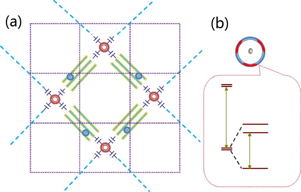
Figure 1: (Color online) (a) Schematic circuit for the resonator lattice, where each TLR is coupled to a single NV center encircled by a PCQ, and the circles denote the central coupler. (b) The subsystem consisting of NV and PCQ, where NV is at the center of the loop. The PCQ is made up of three Josephson junctions, and it couples to the NV via the magnetic field at the center of the loop generated by the persistent currents in the loop. The energy diagram of the NV is shown in the red box.

In this work, we develop an optical system for engineering the strongly correlated effects of light in a hybrid solid-state system. We consider a $2D$ square lattice of coupled TLRs SC , where each TLR is coupled to a single NV NV1 ; QP encircled by a persistent current qubit (PCQ). We show that the competition between the NV-PCQ-TLR interaction and the nonlocal hopping induces the photonic localization-delocalization transition. Subsequently the Mott insulator (MI) phase and the superfluid (SF) phase can appear in a controllable way. The phase boundary in the case of photon hopping with real/complex-valued amplitudes can be obtained using the mean-field approach. Also, the quantum jump technique is employed to describe the phase diagram when the dissipation is considered. Finally, the possibility of observation of the QPT is discussed by employing experimentally accessible parameters.

In our architecture, one can tune independently the on-site emitter-field interaction and the nonlocal photonic hopping between adjacent TLRs. This permits us to systematically study the localization-delocalization transition of light in a complete parameter space. The main motivation for building such a hybrid system is to combine several advantages: in situ tunability of circuit elements Cir3 , spectroscopic technology for state readout, peculiar characteristics of NV (e.g., individual addressing and long coherence time at room-temperature NV2 ), and scalability of TLR arrays Houck ; Koch ; Nu1 ; Nu2 . Recently, D. Underwood et al experimentally fabricated 25 arrays of TLRs and demonstrated the feasibility of quantum simulation in circuit QED system Und . E. Lucero et al experimentally characterized a complex circuit composed of four phase qubits and five TLRs to realize intricate quantum algorithms Lu . The progress renders the TLR lattice a good platform for studying condensed-matter physics with photons and makes our scheme to be more practical.

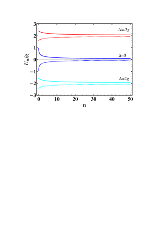
Figure 2: (Color online) The dependence of effective on-site repulsion $U_{\pm}$ on the photon number $n$ under the different detunings $\Delta$, where the solid (dotted) line denotes $U_{+}$ $(U_{-})$.

II Model

As illustrated in Fig. 1, we consider a $2D$ lattice of coupled TLRs, where the basic unit consists of a TLR coupled to a single NV encircled by a PCQ, which acts as an interconnect to greatly magnify the NV-TLR coupling by several orders of magnitude, compared with the direct NV-TLR coupling (far below the linewidth of TLR with dozens of $kHz$) resulting from the vacuum fluctuations of the photons Vac ; Sys . The TLR is made of a superconductor line interrupted by two capacitors at its ends. In the microwave domain, it can be treated as a quantum LC harmonic oscillator, $H^{TLR}=\omega_{r}(a^{+}a+1/2)$ ($\hbar=1$), where $\omega_{r}=\sqrt{1/L_{r}C_{r}}$ is the corresponding eigenfrequency with inductance $L_{r}$ and capacitance $C_{r}$. The PCQ located at an antinode of TLR’s magnetic field is formed by a superconducting loop interrupted by three Josephson junctions Pcq . When the loop is biased by half a magnetic flux quantum, the device is an effective two-level qubit made up of two countercirculating persistent currents with the Hamiltonian $H^{PCQ}=\frac{\omega_{0}}{2}\sigma_{z}$. The NV can be modeled as a three-level system in the triplet ground-state subspace consisting of $\left|{}^{3}A,m_{s}=0\right\rangle$ and $\left|{}^{3}A,m_{s}=\pm 1\right\rangle$. The Hamiltonian is $H^{NV}=\gamma_{e}B_{z}S_{z}+D(S_{z}^{2}-2/3)$, where $\gamma_{e}$ is the electronic gyromagnetic ratio, $D/2\pi\sim 2.87GHz$ is the zero-field splitting, $B_{z}$ is a perpendicular magnetic field at the NV and $S_{z}$ is the spin-1-$z$ operator.

The PCQ magnetically couples to TLR via mutual inductance, $H^{T-P}=-\hat{\mu}\cdot\hat{B}$, where $\hat{\mu}$ is the magnetic dipole of PCQ induced by the persistent circulating currents and $\hat{B}$ is the magnetic field at PCQ induced by the current in the central conductor of TLR. When $\omega_{r}\sim\omega_{0}$, we have $H^{T-P}=g(a^{+}\sigma^{-}+a\sigma^{+})$ after rotating wave approximation, where $g=(I_{p}\mu_{0}r^{2}/d)\sqrt{\omega_{r}/2L_{r}}$, $r$ $(I_{p})$ is the radius (persistent circulating current) of the PCQ loop, and $d$ is the distance between PCQ and central conductor of TLR. The sizable changes of magnetic flux within the loop induced by $I_{p}$ presented in the PCQ lead to small shifts in the transition frequencies ($m_{s}\rightarrow\pm 1$) of NV Sys ; Pcq . Through this small change in magnetic field the PCQ can couple to the NV via Zeeman term, $H^{N-P}=\frac{1}{2}\eta\sigma_{z}S_{z}$, where $\eta=I_{p}\mu_{0}\gamma_{e}/r$.

The basic unit in our system is thus governed by the Hamiltonian $H_{p}^{0}=H^{TLR}+H^{PCQ}+H^{NV}+H^{T-P}+H^{N-P}$. The photonic tunneling in our model can be realized by a central coupler expl1 which serves as individual tunable quantum transducers to transfer photonic states between adjacent TLRs. We have presented a new paradigm for $2D$ TLR lattice coupled to solid-state spins. We have shown that specially engineered resonator lattice provides a practical platform to couple both individual spin and superconducting qubit, and engineer their interactions in a way that surpasses the limitations of current technologies. This can provide new insights to many-body physics.

III Mott-superfluid transition

We study the full Hamiltonian of the $2D$ square lattice by adding the on-site chemical potential and the nonlocal microwave photon hopping between adjacent sites. The Hamiltonian is given by

$$H=\sum_{p}H_{p}^{0}+\sum_{\left\langle p,q\right\rangle}k_{\left\langle p,q\right\rangle}a_{p}^{+}a_{q}-\sum_{p}\mu_{p}N_{p},$$ (1)

where $k_{\left\langle p,q\right\rangle}=$ $2Z_{0}C_{\left\langle p,q\right\rangle}(\omega_{r}+\delta_{p})(\omega_{r}+\delta_{q})$ are photonic tunneling rates between resonators $p$ and $q$, which are set by the tunable mutual capacitance $C_{\left\langle p,q\right\rangle}$ between resonator ends with characteristic impedance $Z_{0}$ and frequency shift $\delta_{p}$ due to random disorder Und . Since $\omega_{r}\gg\delta_{p}$, one can assume that $k_{\left\langle p,q\right\rangle}=k=2Z_{0}C\omega_{r}^{2}$ without disorder for nearest-neighbor resonators, and $k_{\left\langle p,q\right\rangle}$ $=0$ for other resonator pairs. $\mu_{p}$ is the chemical potential at the $p$-th site. The conserved quantity in our system is the total number of excitations $N_{p}=a_{p}^{+}a_{p}+\sigma_{p}^{+}\sigma_{p}^{-}+\frac{1}{2}S_{p}^{+}S_{p}^{-}$ with $S^{i}$ $(\sigma^{i})$ the spin-$1$ (-$1/2$) operators $(i=x,y,\pm)$.

The photon-dependent eigenstates of the Hamiltonian $H_{p}^{0}$ is dressed states $\left|m_{s},\pm,n\right\rangle$ with the eigenvalues $E_{\left|m_{s},\pm,n\right\rangle}=n\omega_{r}+(-\Delta+2n\Delta\pm\sqrt{4ng^{2}+\Delta^{2}\pm 2\Delta\eta+\eta^{2}})/2+\chi(m_{s})$, where $\chi(m_{s})=D(3\times 1^{m_{s}}-2)+m_{s}\gamma_{e}B_{z}$ is the eigenenergy of $H^{NV}$. Here $\Delta=\omega_{r}-\omega_{0}$ is the detuning, $n$ is the number of excitations in the resonator and $|\pm\rangle=$ $(|e\rangle\pm|g\rangle)/\sqrt{2}$. In our case, the dynamics is governed by the Jaynes-Cummings (JC) type of interaction, which enables the interconversion of qubit excitations and photons, and provides the effective on-site repulsion. Meanwhile, pairs of TLRs are coupled by the two-site Hubbard model via one-photon hopping. The difference between the Bose–Hubbard model (BHM) BHM and our model is that the conserved particles are the polaritons rather than the pure bosons in BHM, and the effective on-site repulsion $U_{\pm}(n)=E_{\left|m_{s},\pm,n+1\right\rangle}-E_{\left|m_{s},\pm,n\right\rangle}$ decreases with the growth of photon number, and $U_{\pm}(n)\rightarrow 0$ in the limit of large $n$ and $\Delta=0$, as shown in Fig. 2, while it is a constant in BHM.

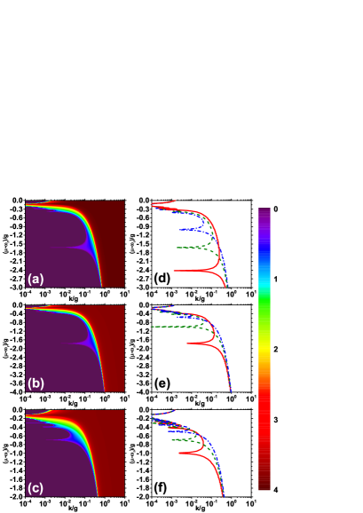
Figure 3: (color online). The phase diagrams in $\mu\sim k$ plane for different sets of NV-PCQ coupling $\eta$ and tunable magnetic fields $B_{z}$ applied on NV, where $\mu$ and $k$ are the chemical potential and the photon hopping rate. The common parameters are $g=1$, $\omega_{r}=200$, $D=100$ and $\gamma_{e}=-10^{3}$. The other parameters are set as (a) $\eta=0.01$, $B_{z}=0.0005T$ and $\Delta=g$, the phase boundaries are plotted in (d), where $\Delta=2g$ (solid), $g$ (dashed) and $0$ (dot-dashed); (b) $\eta=1.2$, $B_{z}=-0.3$ and $\Delta=0$, the phase boundaries are plotted in (e), where $B_{z}=-0.3T$ (solid), $0.0005T$ (dashed) and $0.3T$ (dot-dashed); (c) $\eta=0.75$, $B_{z}=0.3T$ and $\Delta=0$, the phase boundaries are plotted in (f), where $\eta=0.01$ (solid), $\eta=0.75$ (dashed) and $\eta=1.5$ (dot-dashed).

The phase diagrams can be distinguished using the corresponding order parameters. Here we choose the SF order parameter $\psi=\langle a_{p}\rangle$ (set to be real) to differentiate between insulator-like and SF-like states. Using the mean-field theory MF   we decouple the hopping term as $a_{p}^{+}a_{q}=$ $\left\langle a_{p}^{+}\right\rangle a_{q}+a_{p}^{+}\left\langle a_{q}\right\rangle-\left\langle a_{p}^{+}\right\rangle\left\langle a_{q}\right\rangle$, the resulting mean-field Hamiltonian can then be written as a sum over single sites,

$$H^{MF}=\sum_{p}[H_{p}^{0}-zk\psi(a_{p}^{+}+a_{p})+zk\psi^{2}-\mu_{p}N_{p}],$$ (2)

where $z=4$ is the number of nearest neighbours. Noting that $[H^{MF},S_{z}]=0$, therefore, we can treat $S_{z}$ in the mean-field Hamiltonian as a c-number and $S_{z}=\pm 1,0$. Minimizing the ground state energy of the Hamiltonian $H^{MF}$ with respect to $\psi$ for different values of $\mu$ and $k$, we obtain the mean field phase diagram/boundary in the $(\mu,k)$ plane when $\eta$ varies from the weak coupling regime $(\eta\ll g)$ to the strong coupling regime $(\eta>g)$ under the resonant/detuning case. The features of Fig. 3 are rich. The regime where $\psi=0$ corresponds to the stable and incompressible MI lobes characterized by a fixed number of excitations at per site with no variance. In each MI lobe, due to the nonlinearity and anharmonicity in the spectrum originating from the photon blockade effect Blo , the strong emitter-field interaction leads to an effective large polariton-polariton repulsion which freezes out hopping and localizes polaritons at individual lattice sites. By contrast, strong hopping favours delocalization and condensation of the particles into the zero-momentum state, namely, $\psi\neq 0$ indicates a SF compressible phase with the stable ground state at each site corresponding to a coherent state of excitations.

Analogous to the BHM, the physical picture behind is that the MI-SF phase transition results from the interplay between polariton delocalization and on-site repulsive interaction. Therefore, the phase boundary primarily depends on the ratio of the photon-hopping rate to the on-site repulsion rate. When the on-site repulsion dominates over hopping, the system should be in the MI phase, otherwise the system will be in the SF phase. From the expression of the parameter $\eta$ and $g$, we can find that reduction of the size of the PCQ loop will increase $\eta$ but decrease $g$, and the adjustment of the distance $d$ only affects TLR-PCQ interaction. Furthermore, the detuning $\Delta$ is also tunable by varying the magnetic field applied on NV. In Fig. 3, one can find that the size of the MI lobes varies with $\Delta$, with the largest Mott lobes found on resonance.

Further insight to the transition can be gained when the photon hopping with complex-valued amplitude exists in Eq. (1), where the hopping process becomes $-\sum\nolimits_{\left\langle p,q\right\rangle}k_{\left\langle p,q\right\rangle}e^{i\phi_{\left\langle p,q\right\rangle}}a_{p}^{+}a_{q}$ with $\phi_{\left\langle p,q\right\rangle}=-\phi_{\left\langle q,p\right\rangle}$ and we set $k_{\left\langle p,q\right\rangle}=k\text{.}$ We emphasize that this process is possible if the intermediate coupling elements are used to break time-reversal symmetry Houck ; Koch ; Per . The parameter $k_{\left\langle p,q\right\rangle}e^{i\phi_{\left\langle p,q\right\rangle}}$ provides a new regime in the dynamical evolution of the system. The sum of the tunneling phases along a closed loop surrounding the plaquette is $2(\phi_{p+1,q}+\phi_{p,q+1}-\phi_{p,q}-\phi_{p+1,q+1})=2\pi\alpha$, which is actually the flux quanta per plaquette. Assuming that $\alpha$s are all equal, the total Hamiltonian under mean-field approximation reads

$$H_{\alpha}^{MF} = \sum\nolimits_{p}[H_{p}^{0}-zk\psi\cos(2\pi\alpha)(a_{p}^{+}+a_{p})$$ (3)

$$+zk\psi^{2}\cos(2\pi\alpha)-\mu_{p}N_{p}].$$

The results are exhibited in Fig. 4, we find that the boundary line gradually shifts to the right as $\alpha$ enhances in the interval $[0,1/4]$. Because of the spatial variation of tunneling phase, the wave function of a polariton from one lattice site to another acquires a nontrivial phase (Aharonov-Bohm phase) AB , which actually reduces the effective hopping rates.

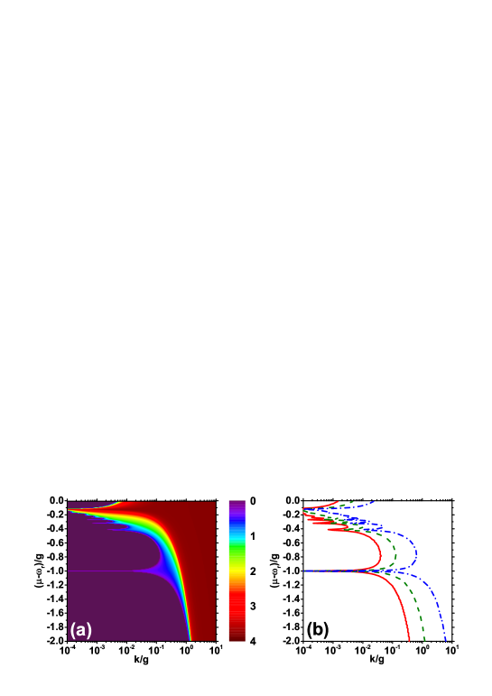
Figure 4: (color online). (a) The order parameter $\psi$ in $\mu\sim k$ plane. The parameters are $g=1$, $\omega_{r}=200$, $D=100$, $\gamma_{e}=-10^{3}$, $\eta=0.01$, $B_{z}=0.0005T$, $\alpha=0.2$, and $\Delta=0$. The corresponding phase boundaries are plotted in (b), where the solid, dashed, and dot-dashed line denote $\alpha=0$, $0.2$, and $0.24$, respectively.

IV Dissipative effects

Generally, nonequilibrium processes such as dissipative effect, are crucial in solid-state devices. We show that the signature of the localization-delocalization transition remains even in the presence of the engineered dissipation by the quantum trajectory method QJ . The non-Hermitian Hamiltonian is formulated as

$$H_{de}=H^{MF}-\frac{i\Gamma}{2}\sum\nolimits_{p}\sigma_{p}^{+}\sigma_{p}^{-}-\frac{i\kappa}{2}\sum\nolimits_{p}a_{p}^{+}a_{p},$$ (4)

where $\kappa=4Z_{0}^{2}C_{out}^{2}\omega_{r}^{3}$ is the decay rate of TLR, and $\Gamma$ is the decay rate from the effective excited state $|e\rangle$ of PCQ. In our case, the dissipative effects result from the unavoidable interaction between the PCQ/TLR and the corresponding Markovian environment, for example, the interaction between the output of the TLR and the corresponding vacuum field will result in a photonic escape rate with $\kappa$ to the continuum. Here the dissipative effects of NV are negligible, compared with $\kappa$ and $\Gamma$. The phase diagrams under dissipative effects are displayed in Fig. 5. Once the hopping rate is increased beyond a critical value, the system is expected to undergo a non-equilibrium QPT from a MI phase, where the initial photon population is self-trapped, to a SF phase with the dynamical photon population imbalance coherently oscillating between pairs of TLRs Houck . Furthermore, another obvious feature is that the size of MI phase becomes larger as the growth of dissipative rates. Note that the effective nonlinearity at per site becomes stronger at lower exciton numbers, which implies that the dissipative effect (inducing the decrease of the exciton numbers) favours the MI phase. As a result, the dissipation results in the dynamical switching from SF phase to MI phase and causes the increment of the size of MI phase.

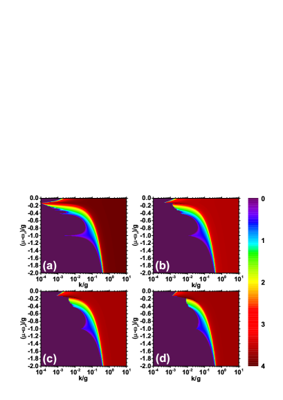
Figure 5: (color online). The order parameter $\psi$ in $\mu\sim k$ plane under the different dissipative rates (a) $\Gamma=\kappa=0.01$; (b) $\Gamma=$ $\kappa=0.05$; (c) $\Gamma=$ $\kappa=0.1$; (d) $\Gamma=\kappa=0.15$. The other parameters are $g=1$, $\omega_{r}=200$, $D=100$, $\gamma_{e}=-10^{3}$, $\eta=0.01$, $B_{z}=0.0005T$, and $\Delta=0$.

V Experimental feasibility

Firstly, we briefly stress the relevant experimental progress. From theoretical standpoint, it is possible to fabricate large arrays to observe many-body physics of interacting polaritons since resonators and qubits can be made lithographically Ash . Actually, it is indeed feasible to couple over $200$ (or 1000) TLRs with negligible disorders (on the order of a few parts in $10^{4}$) in a $2D$ lattice using a $32mm\times 32mm$ sample or a full two-inch wafer Houck . Secondly, how to probe quantum many-body states of light is still an open question in photonic quantum simulation Ma . The previous works ref2 ; Ang suggested to measure the individual TLR through mapping the excitations into the qubit followed by state-selective resonance fluorescence spectrum, but a remaining technical challenge is the realization of high-efficiency photon detectors. Alternatively, the local statistical property of TLR can be analyzed readily using combined techniques of photon-number-dependent qubit transition exper1 ; exper2 and fast readout of the qubit state through a separate low-Q resonator mode read , for which the high-efficiency photon detectors are not required. Experimentally, transmission and reflection measurements for circuit QED arrays have been implemented successfully in small system with one or two resonators Cir1 ; exper2 . Therefore, in order to distinguish between different phases of the system, one can also experimentally probe beyond transmission, such as two-tone spectroscopy and second-order coherence function (photon statistics) to reveal additional information. The tunability of coupling strengths in our system enables one to measure these quantities relatively straightforwardly.

Finally, we survey the relevant experimental parameters. Given the flexibility of circuit QED, we can access a wide range of tunable experimental parameters for TLR-PCQ coupling strength $g$ and hopping rate $k_{\left\langle p,q\right\rangle}$. Taking $L_{r}=2$ $nH$, $\omega_{r}/2\pi=6$ $GHz$, $I_{p}=600$ $nA$, and $r=0.2$ $\mu m$, we get $\eta/2\pi\simeq 140$ $KHz$ and $g/2\pi\sim[1.8,180]$ MHz when the distance $d$ varies from $5$ $\mu m$ to $50$ $nm$. Furthermore, the hopping rate $k_{\left\langle p,q\right\rangle}$ depends on the tunable mutual capacitance $C_{\left\langle p,q\right\rangle}$ between resonator ends. In Ref Und , the authors measured devices with photon hopping rates $k/2\pi$ form $0.8$ MHz to $31$ MHz in resonators lattices. On the other hand, the electron-spin relaxation time $T_{1}$ of NV ranges from 6 ms at room temperature D2 to $28\sim 265$ s at low temperature D3 . In addition, later experimental progress D5 with isotopically pure diamond has demonstrated a longer dephasing time to be $T_{2}$ $=1.8$ $ms$. Therefore, the dissipation and decoherence of NV are negligible.

VI Conclusion

We have devised a concrete hybrid system to engineer photonic MI-SF phase transition in a $2D$ square lattice of TLRs coupled to a single NV encircled by a PCQ. We find that the interplay between the on-site repulsion and the nonlocal tunneling leads to the photonic localization-delocalization transition. In the presence of dissipation, the phase boundary can be obtained by the mean-field approach and the quantum jump technique. Facilitated by high levels of connectivity in circuit QED, experiments combining both scalability and long coherence times are expected in the coming few years, at that stage the investigation of photonic QPT using TLR lattice systems can therefore be easier to realize.

- (1) A. D. Greentree, C. Tahan, J. H. Cole, and C. L. Hollenberg, Nat. Phys. 2, 856 (2006).
- (2) M. J. Hartmann, F. G. S. L. Brandao, and M. P. Plenio, Laser Photonics Rev. 2, 527 (2008); M. J. Hartmann, F. G. S. L. Brandao, and M. P. Plenio, Nat. Phys. 2, 849 (2006).
- (3) M. Fleischhauer, J. Otterbach, and R. G. Unanyan, Phys. Rev. Lett. 101, 163601 (2008); S. Schmidt and G. Blatter, Phys. Rev. Lett. 103, 086403 (2009).
- (4) J. Koch and K. Le Hur, Phys. Rev. A 80, 023811 (2009); S. Schmidt, D. Gerace, A. A. Houck, G. Blatter, and H. E. Türeci, Phys. Rev. B 82, 100507 (2010).
- (5) G. Lepert, M. Trupke, M. J. Hartmann, M. B. Plenio, and E. A. Hinds, New J. Phys. 13, 113002 (2011); W. L. Yang, Zhang-qi Yin, Z. X. Chen, Su-Peng Kou, M. Feng, and C. H. Oh, Phys. Rev. A 86, 012307 (2012); J. Raftery, D. Sadri, S. Schmidt, H. E. Türeci, and A. A. Houck, Phys. Rev. X 4, 031403.
- (6) A. Houck, H. E. Türeci, and J. Koch, Nat. Phys 8, 292 (2012).
- (7) A. Wallraff, D. I. Schuster, A. Blais, L. Frunzio, R.-S. Huang, J. Majer, S. Kumar, S. M. Girvin, and R. J. Schoelkopf, Nature (London) 431, 162 (2004); I. Chiorescu, P. Bertet, K. Semba, Y. Nakamura, C. J. P. M. Harmans and J. E. Mooij, Nature (London) 431, 159 (2004).
- (8) J. Jin, D. Rossini, R. Fazio, M. Leib, and M. J. Hartmann, Phys. Rev. Lett. 110, 163605 (2013); I. M. Georgescu, S. Ashhab, and F. Nori, Rev. Mod. Phys. 86, 153 (2014).
- (9) J. Q. You and F. Nori, Nature (London) 474, 589 (2011); I. Buluta and F. Nori, Science 326, 108 (2009); P. D. Nation, J. R. Johansson, M. P. Blencowe, and Franco Nori, Rev. Mod. Phys. 84, 1 (2012).
- (10) R. Fazio and H. van der Zant, Phys. Rep. 355, 235 (2001).
- (11) M. Lewenstein, A. Sanpera, V. Ahufinger, B. Damski, A. Sen(De), and U. Sen, Adv. Phys. 56, 243 (2007).
- (12) A. Blais, R.-S. Huang, A. Wallraff, S. M. Girvin, and R. J. Schoelkopf, Phys. Rev. A 69, 062320 (2004); R. J. Schoelkopf and S. M. Girvin, Nature 451, 664 (2008); J. Clarke and F. K. Wilhelm, Nature (London) 453, 1031 (2008).
- (13) T. Gaebel, M. Domhan, I. Popa, C. Wittmann, P. Neumann, F. Jelezko, J. R. Rabeau, N. Stavrias, A. D. Greentree, S. Prawer, J. Meijer, J. Twamley, P. R. Hemmer, and J. Wrachtrup, Nat. Phys. 2, 408 (2006); L. Childress, M. V. G. Dutt, J. M. Taylor, A. S. Zibrov, F. Jelezko, J. Wrachtrup, P. R. Hemmer, and M. D. Lukin, Science 314, 281 (2006); M. V. G. Dutt, L. Childress, L. Jiang, E. Togan, J. Maze, F. Jelezko, A. S. Zibrov, P. R. Hemmer, and M. D. Lukin, Science 316, 1312 (2007); X. Zhu, S. Saito, A. Kemp, K. Kakuyanagi, S.-i. Karimoto, H. Nakano, W. J. Munro, Y. Tokura, M. S. Everitt, K. Nemoto, M. Kasu, N. Mizuochi, and K. Semba, Nature (London) 478, 221 (2011).
- (14) T. Hummer, G. M. Reuther, P. Hanggi, and D. Zueco, Phys. Rev. A 85, 052320 (2012).
- (15) L. Jiang, J. S. Hodges, J. R. Maze, P. Maurer, J. M. Taylor, D. G. Cory, P. R. Hemmer, R. L. Walsworth, A. Yacoby, A. S. Zibrov, and M. D. Lukin, Science 326, 267 (2009); P. Neumann, J. Beck, M. Steiner, F. Rempp, H. Fedder, P. R. Hemmer, J. Wrachtrup, F. Jelezko, Science 329, 542 (2010); I. Aharonovich, S. Castelletto, D. A. Simpson, C.-H. Su, A. D. Greentree, and S. Prawer, Rep. Prog. Phys. 74, 076501 (2011).
- (16) J. Koch, A. A. Houck, K. L. Hur, and S. M. Girvin, Phys. Rev. A 82, 043811 (2010); A. D. Greentree and A. M. Martin, Physics, 3, 85 (2010); A. Nunnenkamp, J. Koch, and S. M. Girvin, New J. Phys. 13, 095008 (2011).
- (17) M. Mariantoni, H. Wang, R. C. Bialczak, M. Lenander, E. Lucero, M. Neeley, A. D. O’Connell, D. Sank, M. Weides, J. Wenner, T. Yamamoto, Y. Yin, J. Zhao, J. M. Martinis, and A. N. Cleland, Nat. Phys. 7, 287 (2011).
- (18) M. Neeley, R. C. Bialczak, M. Lenander, E. Lucero, M. Mariantoni, A. D. O’Connell, D. Sank, H. Wang, M. Weides, J. Wenner, Y. Yin, T. Yamamoto, A. N. Cleland, and J. M. Martinis, Nature (London) 467, 570 (2010); L. DiCarlo, M. D. Reed, L. Sun, B. R. Johnson, J. M. Chow, J. M. Gambetta, L. Frunzio, S. M. Girvin, M. H. Devoret, and R. J. Schoelkopf, Nature (London) 467, 574 (2010).
- (19) D. L. Underwood, W. E. shanks, J. Koch, and A. A. Houck, Phys. Rev. A 86, 023837 (2012).
- (20) E. Lucero, R. Barends, Y. Chen, J. Kelly, M. Mariantoni, A. Megrant, P. O’Malley, D. Sank, A. Vainsencher, J. Wenner, T. White, Y. Yin, A. N. Cleland, and J. M. Martinis, Nat. Phys. 8, 719 (2012).
- (21) A. A. Abdumalikov, J. O. Astafiev, Y. Nakamura, Y. A. Pashkin, and J. Tsai, Phys. Rev. B 78, 180502 (2008).
- (22) J. Twamley and S. D. Barrett, Phys. Rev. B 81, 241202(R) (2010).
- (23) T. P. Orlando, J. E. Mooij, L. Tian, C. H. van der Wal, L. S. Levitov, S. Lloyd, and J. J. Mazo, Phys. Rev. B 60, 15398 (1999).
- (24) Here, the central coupler may be conceived as a Josephson ring circuit Koch , or a current-biased Josephson junction phase qubit CBJJ , or a capacitive coupling element Hu , or an active non-reciprocal devices as proposed in Kam .
- (25) Y. Yu, S. Han, X. Chu, S.-I. Chu, Z. Wang, Science 296, 889 (2002); J. M. Martinis, S. Nam, J. Aumentado, and C. Urbina, Phys. Rev. Lett. 89, 117901 (2002); A. Blais, A. Brink, and A. M. Zagoskin, Phys. Rev. Lett. 90, 127901 (2003); A. M. Zagoskin, S. Ashhab, J. R. Johansson, and F. Nori, Phys. Rev. Lett. 97, 077001 (2006).
- (26) Y. Hu and L. Tian, Phys. Rev. Lett. 106, 257002 (2011).
- (27) A. Kamal, J. Clarke, and M. H. Devoret, Nat. Phys. 7, 311 (2011).
- (28) T. D. Kühner, S. R. White, and H. Monien, Phys. Rev. B 61, 12474 (2000).
- (29) D. van Oosten, P. van der Straten, and H. T. C. Stoof, Phys. Rev. A 63, 053601 (2001); D. van Oosten, P. van der Straten, and H. T. C. Stoof, Phys. Rev. A 67, 033606 (2003).
- (30) K. M. Birnbaum, A. Boca, R. Miller, A. D. Boozer, T. E. Northup, and H. J. Kimble, Nature (London) 436, 87 (2005); C. Lang, D. Bozyigit, C. Eichler, L. Steffen, J. M. Fink, A. A. Abdumalikov, Jr., M. Baur, S. Filipp, M. P. da Silva, A. Blais, and A. Wallraff, Phys. Rev. Lett. 106, 243601 (2011); A. J. Hoffman, S. J. Srinivasan, S. Schmidt, L. Spietz, J. Aumentado, H. E. Türeci, and A. A. Houck, Phys. Rev. Lett. 107, 053602 (2011).
- (31) B. Peropadre, D. Zueco, F. Wulschner, F. Deppe, A. Marx, R. Gross, and J. J. García-Ripoll, Phys. Rev. B 87, 134504 (2013).
- (32) Y. Aharonov and D. Bohm, Phys. Rev. 115, 485 (1959); Y. Aharonov and D. Bohm, Phys. Rev. 123, 1511 (1961).
- (33) M. B. Plenio and P. L. Knight, Rev. Mod. Phys. 70, 101 (1998); H. Carmichael, An Open Systems Approach to Quantum Optics (Springer-Verlag, Berlin, 1993).
- (34) D. Tsomokos, S. Ashhab, and F. Nori, Phys. Rev. A 82, 052311 (2010).
- (35) D Marcos, A Tomadin, S Diehl, and P Rabl, New. J. Phys. 14, 055005 (2012).
- (36) D. G. Angelakis, M. F. Santos, and S. Bose, Phys. Rev. A 76, 031805 (2007).
- (37) D. I. Schuster, A. A. Houck, J. A. Schreier, A. Wallraff, J. M. Gambetta, A. Blais, L. Frunzio, J. Majer, B. Johnson, M. H. Devoret, S. M. Girvin, and R. J. Schoelkopf, Nature (London) 445, 515 (2007).
- (38) B. R. Johnson, M. D. Reed, A. A. Houck, D. I. Schuster, Lev S. Bishop, E. Ginossar, J. M. Gambetta, L. DiCarlo, L. Frunzio, S. M. Girvin, and R. J. Schoelkopf, Nat. Phys. 6, 663 (2010).
- (39) P. J. Leek, M. Baur, J. M. Fink, R. Bianchetti, L. Steffen, S. Filipp, and A. Wallraff, Phys. Rev. Lett. 104, 100504 (2010).
- (40) For instance, by driving the first TLR with a microwave source and detecting the output field of the last TLR, we could probe the properties of the system by independently detecting the correlation between distant sites.
- (41) P. Neumann, N. Mizuochi, F. Rempp, P. Hemmer, H. Watanabe, S. Yamasaki, V. Jacques, T. Gaebel, F. Jelezko, and J. Wrachtrup, Science 320, 1326 (2008).
- (42) J. Harrison, M. J. Sellars, and N. B. Manson, Diam. Relat. Mater. 15, 586 (2006).
- (43) G. Balasubramanian, P. Neumann, D. Twitchen, M. Markham, R. Kolesov, N. Mizuochi, J. Isoya, J. Achard, J. Beck, J. Tissler, V. Jacques, P. R. Hemmer, F. Jelezko, and J. Wrachtrup, Nat. Mater. 8, 383 (2009).