Fixed curves near fixed points
Abstract.
Let be a composition of an -linear planar mapping and . We classify the dynamics of in terms of the parameters of the -linear mapping and the degree by associating a certain finite Blaschke product. We apply this classification to this situation where is a fixed point of a planar quasiregular mapping with constant complex dilatation in a neighbourhood of . In particular we find how many curves there are that are fixed by and that land at .
1. Introduction
1.1. Background
Complex dynamics has been a field of intense study over the last thirty years. The striking computer generated images of the Mandelbrot set helped inspire this surge of activity and showed how very complicated behaviour can arise from very simply defined iterative systems. Yet complex dynamics had its first burst of interest at the end of the nineteenth and into the beginning of the twentieth centuries. Koenigs and Böttcher classified the behaviour of holomorphic functions near fixed points by conjugating to simpler functions. In a neighbourhood of a fixed point, a holomorphic function can be conjugated to either or depending on whether or not the holomorphic function is injective in a neighbourhood of the fixed point. See Milnor’s book [19] for an exposition of these ideas.
Quasiconformal mappings and quasiregular mappings provide natural higher dimensional analogues for holomorphic functions in the plane. Informally speaking, quasiregular mappings are mappings which allow a bounded amount of distortion. They share many value distributional properties with holomorphic functions, for example versions of Picard’s and Montel’s Theorems hold, but they are more flexible than holomorphic functions. The only holomorphic functions in for are Möbius transformations, and so it is natural to allow distortion to have an interesting function theory. See Rickman’s book [22] for an introduction to the theory of quasiregular mappings.
Much more is known about quasiregular mappings in the planar setting: every quasiregular mapping has a Stoilow decomposition, that is, it can be written as a composition of a holomorphic function and a quasiconformal mapping. The holomorphic part takes care of the branching and the quasiconformal part takes care of the distortion. The main reason that more is known in the plane is due to the Measurable Riemann Mapping Theorem, which states that solutions of the Beltrami differential equation for with are quasiconformal mappings which can be assumed to fix and . Conversely, given a quasiconformal mapping , its complex dilatation is contained in the unit ball of .
The Measurable Riemann Mapping Theorem was used by Douady and Hubbard, and Sullivan to great effect in the 1980s in proving fundamental results in complex dynamics. See Branner and Fagella’s book [6] for a survey of the use of quasiconformal and quasiregular methods in modern complex dynamics.
More recently, there has been an interest in studying the iteration of quasiregular mappings themselves. A composition of quasiregular mappings is again quasiregular. However, the distortion of the iterates of a quasiregular mapping will typically increase. This means the machinery available from Montel’s Theorem is unavailable to help with the iterative theory. Remarkably, it is still possible to say quite a lot about the dynamics of quasiregular mappings when there is not a uniform bound on the distortion of the iterates. See for example the recent works of Bergweiler [2, 3].
1.2. Overview of the paper
In section 2, we will recall the definition of quasiconformal and quasiregular mappings, with focus on the planar case. Taking as an inspiration the work of Douady and Hubbard in studying the simplest non-trivial polynomials , an initial step for studying quasiregular mappings in the plane is to study those which are the simplest: using the Stoilow decompostion, these are mappings which can be written as a composition of a power of and a quasiconformal mapping of constant complex dilatation. These were first studied in [11] and in more detail for the degree two case in [13]. We remark that similar quasiregular perturbations of polynomials were studied in [4, 5, 7, 20, 21].
By construction, every such mapping maps rays emanating from onto rays and so every such mapping induces a degree circle endomorphism. The major insight here is that such a circle map is strongly related to a particular Blaschke product and the dynamics of the Blaschke product has strong implications for the dynamics of the original quasiregular mapping.
In particular, every fixed point of the Blaschke product corresponds to either a fixed ray of the quasiregular mapping or a pair of opposite rays which switch. Here, the cases of even or odd are different. Further, the Julia set of a Blaschke product is either the whole circle or a Cantor subset of it. We classify the type of the quasiregular mapping in terms of the complex dilatation by relating it to the parameter space of degree unicritical Blaschke products.
We next show that for such quasiregular mappings, the plane breaks into three dynamically interesting sets: the basins of attraction of and respectively and the boundary between them. We show that as long as the distortion is smaller than the degree, the boundary is the Julia set of the quasiregular mapping. Otherwise there are cases when the boundary of basins of attraction fails to have the necessary blowing-up property required for the Julia set.
An important point in the analysis of these mappings is that they are not uniformly quasiregular. For otherwise they would just be quasiconformal conjugates of holomorphic mappings and this study would not be of independent interest. We will show that in fact the distortion of the iterates blows up at every point for such mappings.
Finally, we show how to construct a Böttcher type coordinate for a fixed point of a quasiregular mapping for which the complex dilatation is constant in a neighbourhood of the fixed point. This allows the results from the rest of the paper to be applied locally.
See [12] for the degree case of such a Böttcher coordinate.
2. Quasiregular mappings with constant complex dilatation
2.1. Quasiregular mappings
We first recall the definitions of quasiconformal and quasiregular mappings in the plane.
A quasiconformal mapping is a homeomorphism so that is in the Sobolev space and there exists such that the complex dilatation satisfies
almost everywhere in . See for example [14] for more details on quasiconformal mappings. The distortion of at is
A mapping is called -quasiconformal if almost everywhere. The smallest such constant is called the maximal dilatation and denoted by . The case corresponds to biholomorphic mappings and so is a way of measuring how far from a conformal mapping is.
If we drop the assumption on injectivity, then is a quasiregular mapping. See for example [16, 22] for the theory of quasiregular mappings. Every quasiregular mapping is locally quasiconformal away from the branch set, which in the planar case is discrete. We can therefore consider the complex dilatation of a quasiregular mapping. In the plane, every quasiregular mapping has an important factorization.
Theorem 2.1 (Stoilow factorization, see for example [16] p.254).
Let be a quasiregular mapping. Then there exists an holomorphic function and a quasiconformal mapping such that .
In this decomposition, the holomorphic part takes care of the branching and the quasiconformal part deals with the distortion.
We call a quasiregular mapping uniformly quasiregular if there exists such that for all . The dynamics of uniformly quasiregular mappings in the plane are well understood due to results of Hinkkanen [15] and Sullivan [23] that state that every uniformly quasiregular map is quasiconformally conjugate to a holomorphic map.
2.2. -linear mappings
Let and . Denote by the -linear mapping
| (2.1) |
This mapping stretches by a factor in the direction . This is a quasiconformal mapping and its complex dilatation is the constant
Every quasiconformal mapping with constant complex dilatation can be written as for some and where is a Möbius transformation (see [13, Proposition 1.1]).
2.3. Quasiregular mappings with constant complex dilatation
Let with and define by
| (2.2) |
This is the mapping whose dynamics will be studied in this paper. We refer to [13] for an analysis of the case. Here, however, we will give a unified treatment for all and classify the behaviour of mappings given by (2.2) into classes which depend on and .
A ray is a semi-infinite line of the form . Since and map rays to rays, so does . Since maps rays to rays, it induces a degree circle endomorphism that we will denote by .
Proposition 2.2.
3. Circle endomorphisms and Blaschke products
In this section, we will show how is related to a Blaschke product. First of all, since is an orientation preserving degree mapping of it is a circle endomorphism. Every circle endomorphism of degree can be lifted to a mapping which satisfies
Definition 3.1.
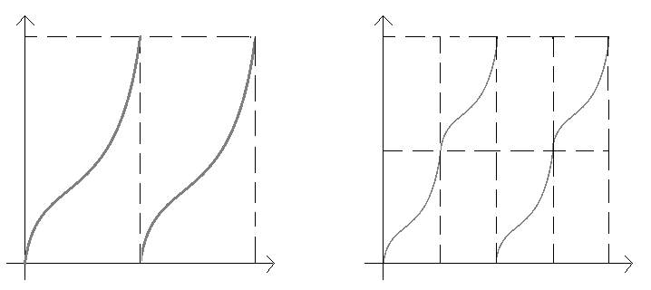
Given a circle endomorphism of degree , consider its lift to . Then we define to be the degree endomorphism whose lift to is given in by
The map is well-defined and essentially rescales by a factor . We can view informally as the conjugate of by , since by construction. See Figure 1 for a diagram showing how and are related on .
Theorem 3.2.
Let for , and . The map agrees with the function , where is the Blaschke product defined by
| (3.1) |
and where .
3.1. Blaschke products
Before proving Theorem 3.2, we will review some of the properties of Blaschke products and, in particular, dynamical aspects we will need.
Recall that a finite Blaschke product is a function given by
| (3.2) |
for some and for . We call a Blaschke product non-trivial if it is not a Möbius mapping, that is, if . For a finite Blaschke product, and are all completely invariant.
Every finite degree self-mapping of is a finite Blaschke product [1, p.19], and so they can be viewed as analogues for polynomials in the disk. By the Schwarz-Pick Lemma, can have at most one fixed point in . If is a fixed point of , then it is straightforward to show that is also a fixed point of . Hence all but possibly two (with the convention that infinity is a fixed point if some ) of the fixed points of must lie on .
The Denjoy-Wolff Theorem [19, p.58] states that if is holomorphic and not an elliptic Möbius mapping then there is some point such that for every . We call such a point a Denjoy-Wolff point of .
Using the Denjoy-Wolff Theorem, there is a classification of finite Blaschke products in analogy with that for Möbius transformations:
-
(i)
is called hyperbolic if the Denjoy-Wolff point of lies on and ,
-
(ii)
is called parabolic if the Denjoy-Wolff point of lies on and ,
-
(iii)
is called elliptic if the Denjoy-Wolff point of lies in . In this case, we must have .
It is not hard to see that the Julia set of a Blaschke product must be contained in and is either the whole of or a Cantor subset of . We summarize the classification of Blaschke products in terms of the Julia set as follows, see for example [9].
Theorem 3.3 ([9]).
Let be a non-trivial finite Blaschke product. Then if and only if is elliptic or is parabolic and , where is the Denjoy-Wolff point of on . On the other hand, is a Cantor subset of if and only if is hyperbolic or is parabolic and .
The class of Blaschke products we will be interested in in this paper are the unicritical Blaschke products, namely those with one critical point in . For , we define the set
of normalized unicritical Blaschke products of degree , which is parameterized by the sector
We denote by those parameters in which give elliptic unicritical Blaschke products and by those parameters in which give rise to unicritical Blaschke products with connected Julia set. We further denote by the set
where is the rotation through angle , and denote by the corresponding set for . The following theorem summarizes results in [10].
Theorem 3.4 ([10]).
Let .
-
(i)
Every unicritical Blaschke product of degree is conjugate by Möbius mappings to a unique element of .
-
(ii)
The connectedness locus consists of and one point on the relative boundary in where .
-
(iii)
The set is a starlike domain about which contains the disk .
-
(iv)
The set consists of and points on its relative boundary in .
-
(v)
If is even, then the ray is contained in for where . The ray is contained in for where .
-
(vi)
If is odd, then the ray is contained in for where . The ray is contained in for where .
We remark that the boundary curve of has recently been shown to be an epicycloid in with cusps, see [8].
3.2. Connection between and Blaschke products
Proof of Theorem 3.2.
Recall from (2.3) that . Writing this using the exponential function yields
Rearranging this in terms of , we obtain
where . We therefore see that
Therefore is obtained by taking the Blaschke product
restricted to , lifting this circle endomorphism to , conjugating by and projecting back to . In summary, as claimed. ∎
We remark here that the cases where is even or odd differ. When is even, is the Blaschke product
However, when is odd, is no longer a Blaschke product because is not an integer.
3.3. Classification of and fixed rays
We can classify the mappings in terms of the associated Blaschke product .
Definition 3.5.
Let , , and . Denote by the associated Blaschke product given by (3.1) where . Then we call elliptic, parabolic or hyperbolic if is elliptic, parabolic or hyperbolic respectively.
Since maps rays to rays, it is of interest to find which rays are fixed by . Fixed rays of correspond to fixed points of and these have a relation to the fixed points of .
3.3.1. Even degree
In this subsection, we assume that is even.
Lemma 3.6.
With the notation above, if is even then there is a one-to-one correspondence between fixed points of on and fixed points of .
Proof.
Let be even. Then . Since by Theorem 3.2, we have . Suppose fixes and . Then
and so . Since maps antipodal points onto the same image, this means that one of and is fixed by and the other is mapped onto this fixed point. On the other hand, if is fixed by , then it is easy to see that is fixed by . Hence and have the same number of fixed points. ∎
Theorem 3.7.
Let be even, , and let . Then is elliptic, parabolic or hyperbolic according to whether , the relative boundary of in or respectively. Further, if are fixed, there exists such that
-
(i)
for , is elliptic and has fixed rays;
-
(ii)
for , is parabolic and has at most fixed rays;
-
(iii)
for , is hyperbolic and has fixed rays.
Proof.
The first part of this theorem is Theorem 3.4 applied to the situation with . Using the fact that is starlike with respect to , if is fixed, then there exists such that if then is elliptic, if then is parabolic, and if then is hyperbolic.
If is elliptic, then has a unique fixed point in , a unique fixed point in and fixed points on . If is hyperbolic then it has fixed points on and so has fixed rays. If is parabolic, then has at most fixed points on . The claims then follow from Lemma 3.6. ∎
3.3.2. Odd degree
In this subsection, we assume that is odd. This case is a little more involved than the even case, because here fixed points of may not correspond to fixed points of .
Lemma 3.8.
With the notation as above, if is odd, then there is a one-to-one correspondence between fixed points of and pairs of antipodal points on which are either both fixed by or switched by . Further,
Proof.
Let be odd. Then . As in the proof of Lemma 3.6, if is fixed by , then is fixed by . However, we also have that if , then is fixed by . On the other hand, if is fixed by and then we again conclude that . However, since is odd, there are two possibilities: either and are both fixed points of or they are switched by . The claim then follows. ∎
Lemma 3.9.
Let be an odd degree circle endomorphism with and fixed points with . For denote by the arc between and , where we identify with . Then either maps onto bijectively or maps onto by wrapping around exactly once. In the first case, this can only happen if one endpoint of is an attracting or neutral fixed point of and no point in can be mapped on its antipode. In the second case, there is at least one point in which maps onto its antipode.
Proof.
With the hypotheses as above, either covers with multiplicity or in which case we take . With this set-up, we have
| (3.3) |
Suppose that some . Then the pre-image consists of disjoint intervals, two of which have endpoints coinciding with the endpoints of . Hence at least one of these pre-images, say , does not have an endpoint coinciding with an endpoint of . Then with contained in the interior of and so there is a fixed point of contained in . This contradicts the fact that there are no fixed points between and and so we conclude that can only be or .
If then there are no points in which are switched under . If both endpoints of are repelling fixed points of , then there exists an arc whose closure is contained in the interior of and so that . Therefore must have another fixed point in the interior of , which is a contradiction. Hence one of the endpoints is not repelling.
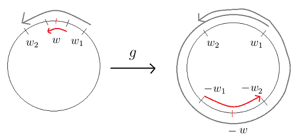
If , then as above is contained in the interior of , where . Therefore there exists at least one point in such that , see Figure 2. This completes the proof.
∎
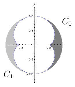
If is odd, then consists of an even number of components which we denote by for taken anticlockwise from the positive real axis. It follows from Theorem 3.4 (vi) that contains a ray from to , see Figure 3.
Theorem 3.10.
Let be odd, , and let .
-
(i)
If , then is elliptic and has fixed rays and switched rays.
-
(ii)
If is in the relative boundary of in , then is parabolic and there are two subcases:
-
(a)
If is on the boundary of for even, then the Denjoy-Wolff point of corresponds to a pair of rays fixed by .
-
(b)
If is on the boundary of for odd, then the Denjoy-Wolff point of corresponds to a pair of rays switched by .
-
(a)
-
(iii)
If , then is hyperbolic and there are again two subcases:
-
(a)
If for even, then the Denjoy-Wolff point of corresponds to a pair of rays fixed by . There are fixed rays and switched rays of .
-
(b)
If for odd, then the Denjoy-Wolff point of corresponds to a pair of rays switched by . There are fixed rays and switched rays of .
-
(a)
Further, if are fixed, there exists such that
-
(i)
for , is elliptic and has fixed rays;
-
(ii)
for , is parabolic and has at most fixed rays;
-
(iii)
for , is hyperbolic and has either or fixed rays, depending on whether for odd or even.
Note that in the parabolic case, may have less than fixed points, so will correspondingly have less fixed and switched rays. For example, is parabolic and has only one fixed point on at .
Proof of Theorem 3.10.
First, if , then is elliptic and every fixed point on is repelling. By Lemma 3.9, for every interval we are in the case. Hence there are fixed rays and switched rays of .
Next, if , then is in some component . Since varying the parameters in moves fixed points of and fixed rays of continuously, it is enough to check what happens on the ray with argument . To that end, let , , recalling that the argument of is , and consider and with parameter . It is not hard to check that
and so is fixed by . Further,
and so this is the Denjoy-Wolff point of . The next question is whether the corresponding rays of , with argument and are fixed or switched by . We have
Therefore if is even, the rays are fixed and if is odd, the rays are switched.
Suppose is even and these rays are fixed. Then applying Lemma 3.9 to , we see that has a pair of attracting fixed points and the rest are repelling and so there are two intervals where , and for the others we must have . Hence by Lemma 3.8 and using the fact has fixed points in this case, has fixed points and switched points.
Similarly, if is odd, then has fixed points and switched points. The parabolic case is similar and so we omit the proof. ∎
Example 3.11.
To illustrate the case when is odd, consider the example , where first and . Then there are fixed points of , including the two attracting fixed points arising from the Denjoy-Wolff point of . The immediate attracting domains are bounded by the other pairs of fixed points. The points are switched by .
On the other hand, if and , then now are the points arising from the Denjoy-Wolff point of . They are still switched by and now the immediate attracting region is bounded by pairs of points which are also switched. This means that are the only fixed points.
4. Attracting and repelling fixed rays
4.1. Density of pre-images
We may classify fixed rays of as attracting, repelling or neutral depending on whether the corresponding fixed point of is attracting, repelling or neutral. This classification also holds for opposite rays that are switched by .
Definition 4.1.
Suppose that . Then the corresponding Blaschke product from (3.1) has a Denjoy-Wolff point . If is even, define to be the corresponding fixed ray with argument and denote by the basin of attraction of , that is,
In this case, we will call the Denjoy-Wolff ray of .
If is odd, then the Denjoy-Wolff point of corresponds to a pair of opposite rays with arguments and which are either both fixed or both swapped by . In this case, the basin of attraction is
The immediate basin of attraction is the component of that contains in even degree case or the two components of that contain and in the odd degree case. Recall the connectedness locus in parameter space of unicritical Blaschke products, and that the Blaschke product of form (3.1) has parameter .
Theorem 4.2.
Let , , and . If and , then for any ray , is dense in . On the other hand, if , then is dense in , where is the basin of attraction defined above.
This theorem can be interpreted as saying either the backward orbit of a ray is dense, or the backward orbit of is dense depending on whether or not . To prove this we first need a result on circle endomorphisms.
4.2. Relating the dynamics of a circle endomorphism to that of
We need to study how the dynamics of the Blaschke product on and the dynamics of are related. By Theorem 3.2, and so if then we have the functional equation .
Definition 4.3.
Let be a degree endomorphism. For such a map, define to be the set of such that for all neighbourhoods of , there exists such that . Further, define to be the complement of in , that is, the set of such that there exists a neighbourhood of such that for all , omits an exceptional set containing at least one point.
Clearly, the exceptional set contains , as long as is non-empty. If is the restriction of a finite Blaschke product to , then and are the Julia set and the Fatou set restricted to respectively.
Lemma 4.4.
We have .
Proof.
First suppose that . Then given any neighbourhood of , there exists such that . Let and find a neighbourhood of so that contains the component of containing . Then . Using the functional equation, this means that . Since is an arc, this means that contains an arc of length . Hence and so .
On the other hand, suppose that . Then there exists a neighbourhood of so that for every , omits an exceptional set . Let and find a neighbourhood of so that is contained in the component of containing . Then . Again using the functional equation, this means that and hence , which contains at least two points. Since this is true for every , . ∎
Denote by the backward orbit of with respect to .
Lemma 4.5.
If , then .
Proof.
Let , and be any neighbourhood of . Then there exists such that . In particular, it follows that there exists with . This proves the lemma. ∎
We can now prove Theorem 4.2.
Proof of Theorem 4.2.
First suppose that . Then by definition . Since , then Lemma 4.4 implies that . Further, Lemma 4.5 implies that if then is dense in . Interpreting this in terms of , the backward orbit of any ray under is dense in .
Next, if , then is a Cantor subset of and there is a Denjoy-Wolff point so that if then . Lemma 4.4 implies that is also a Cantor subset of and so is dense in . The Denjoy-Wolff point of corresponds to either a single fixed ray or a pair of rays that are either fixed or switched by , as discussed above. Interpreting this in terms of , the basin of attraction is dense in . ∎
5. Decomposition of the plane
5.1. Attracting basins and their boundary
The dynamics of break up the plane into three dynamically interesting sets.
Theorem 5.1.
Let be as in (2.2). Then the attracting basin of , , is star-like about and we may write
where denotes the escaping set. In other words, the attracting basins of and respectively form two completely invariant domains with boundary a Jordan curve.
Proof of Theorem 5.1.
Fix , , and let be defined by (2.2). By [11, Theorem 4.3], since is a composition of a bi-Lipschitz map and a polynomial, the escaping set is a connected, completely invariant, open neighbourhood of infinity and is a completely invariant closed set. It is clear that is a topologically attracting fixed point of and so the basin of attraction is completely invariant and open.
Let be a fixed ray of . Then on , we have
where by the polar form (2.3) of . For , this point is fixed, for the point is in and for , the point is in . By complete invariance, any pre-image of breaks up into and in the same way.
Suppose that so that . Then by Theorem 4.2, if is any fixed ray of , its pre-images under are dense in . Since and are open, this proves the result in this case.
Next, if , then is a Cantor subset of and is dense in . By Theorem 4.2, the basin of attraction is dense in . Suppose first that is even and that . Then where is the attracting fixed ray. Since and are open, it is not hard to see that decomposes in the same way that does. Since is dense in , the openness of and again imply the result in this case.
The case where is odd and the Denjoy-Wolff point of corresponds to a pair of rays which are either fixed or switched follows similarly by considering . This sequence converges to or and we then proceed as above. ∎
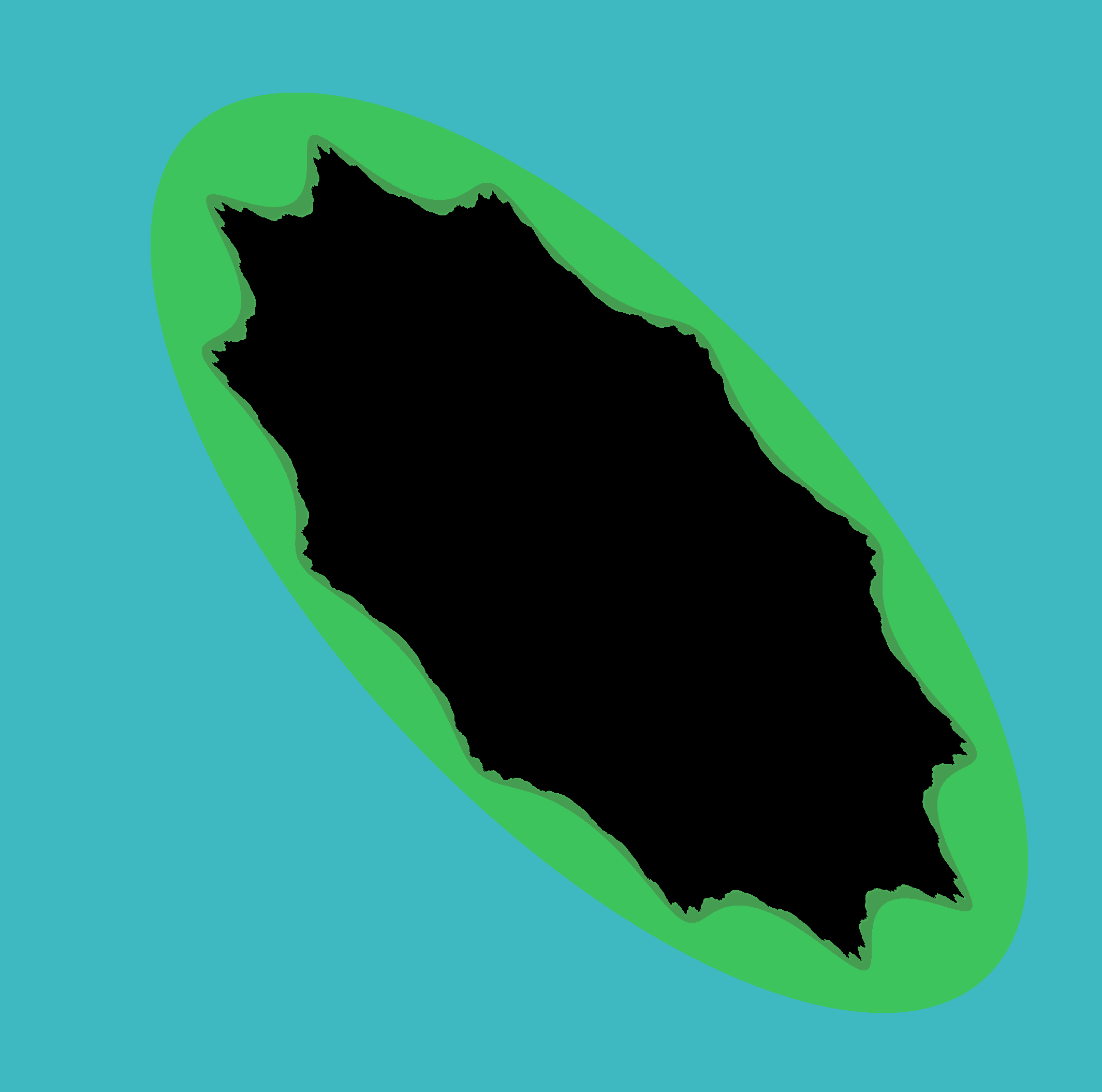
It would be interesting to know the regularity of . For example, is it a quasi-circle? See the computer pictures generated by Doug Macclure in Figures 4 and 5 for examples.
5.2. Julia sets
In [3], the Julia set for quasiregular mappings of polynomial type is defined, but only when the degree is larger than the distortion. For such mappings, is defined by
where denotes the forward orbit of the set . We omit the definition of capacity zero here, but remark that such sets must be necessarily of Hausdorff dimension zero [22, Corollary VII.1.16]. We next show that all such mappings to which this definition of the Julia set applies are elliptic.
Proof.
This follows immediately from Theorem 3.4 (iii), that contains an open disk of radius , and the fact that . ∎
This shows that the Julia set definition can only apply when is elliptic. It follows fairly straightforwardly that in fact if then all points on have the blowing-up property of the Julia set and by Theorem 5.1 these are the only such points.
On the other hand, if , then there are points on without the blowing-up property in the Julia set definition. In fact, the only points with the blowing-up property are those on that arise from the Julia set of , which we recall is a Cantor set. This gives another class of examples where the boundary of the escaping set and the set with a blowing-up property do not agree, c.f. [2].
6. Unbounded distortion of the iterates
6.1. Nowhere uniform quasiregularity
The dynamics of mappings of the form are only of independent interest if the distortion of the iterates is unbounded. This is because every uniformly quasiregular mapping of the plane is a quasiconformal conjugate of a holomorphic mapping. This means that the iteration of uniformly quasiregular mappings of the plane yields nothing new compared to complex dynamics. We will next show that mappings of the form satisfy a condition that is slightly stronger than not being uniformly quasiregular. We recall the following definition from [13].
Definition 6.1.
Given a plane domain , a quasiregular mapping is called nowhere uniformly quasiregular if for every , we have is unbounded as , where
where denotes the distortion of at and the infimum is taken over all neighbourhoods of .
For example, the quasiconformal mapping is easily seen to be nowhere uniformly quasiregular for any .
Theorem 6.2.
Let , and . Then is nowhere uniformly quasiregular.
Before proving this, we need to recall some material on Möbius transformations.
6.2. Möbius transformations
Every Möbius transformation of the unit disk can be written in the form
The mapping can be represented by the matrix which has trace-squared . The value of classifies the dynamical behaviour of :
-
(i)
if then is elliptic and there exists a fixed point ;
-
(ii)
if , then is parabolic and there exists one fixed point ;
-
(iii)
if , then is hyperbolic and there exist two fixed points in .
We will need the following theorem on the composition of varying Möbius maps.
Theorem 6.3.
[18] Let be hyperbolic Möbius maps of such that as for all and locally uniformly as . Suppose we have a sequence of hyperbolic Möbius maps of defined by
Then as for all .
6.3. On fixed rays and switched rays
We now show that if is on a fixed ray of or a pair of switched rays, then the distortion of the iterates of is unbounded.
Recall that the complex dilatation of a quasicregular mapping is given by
The composition formula for complex dilatations is (see for example [14]):
| (6.1) |
where . Hence , we see that is the constant
Lemma 6.4.
For ,
Next, if is on a fixed ray of , then , where is the Möbius transformation
for some . Finally, if is on a pair of rays switched by , then , where is the Möbius transformation
for some .
Proof.
For the first part, we just need to calculate and apply (6.1) to . We can calculate that
| (6.2) |
from which it follows that .
Next, suppose that is fixed by and . Since , we must have for some . Hence is constant on and it follows by induction that must be constant on and given by the desired iterated Möbius map evaluated at .
For the final case, if and are switched by and say , then and so for some . Since maps pairs of opposite rays onto pairs of opposite rays, if , then . Hence for on either of the swapped rays, we have , and the claim follows. ∎
Suppose that is a fixed ray of . Then there is an associated Möbius map given by in Lemma 6.4 which we can write as
where and . The point is that the matrix representing this latter way of writing has determinant and has trace-squared equal to
| (6.3) |
Since Möbius transformations and their dynamical behaviour are classified by , we can use to get information about how behaves on .
Lemma 6.5.
Let be a fixed ray of . Then, with as above,
Hence is parabolic or hyperbolic and consequently for any .
Proof.
Using (6.3),
as claimed. We have to show that this expression is always at least . To that end, if is a fixed ray, then
| (6.4) |
Next, (6.4) and the tangent addition formula give
Consider the function
An elementary calculation shows that . Then since , we get
Hence by the classification of Möbius transformations, is parabolic or hyperbolic. This means that there exists such that for every , . ∎
This shows that on fixed rays, is nowhere uniformly quasiregular. The case for switched rays follows analogously with replaced with , recalling Lemma 6.4.
6.4. Everywhere else
To show that is nowhere uniformly quasiregular everywhere, we combine Lemma 6.5 with Theorem 4.2 on the density of either the pre-images of a fixed ray if , or the density of the basin of attraction otherwise.
We deal first with the case that .
Lemma 6.6.
Suppose that . Then is nowhere uniformly quasiregular.
Proof.
Let be a fixed ray of and fix . Then is dense in by Theorem 4.2. If lies on a ray then there exists such that . That is, lies on the ray for . We can apply (6.1) to obtain:
| (6.5) |
for , where . Notice that and that if we define
| (6.6) |
then is a Möbius map of the disk and further we see that
for . Using the fact that for , (6.6) and Lemma 6.5 we see that (6.5) becomes
| (6.7) |
for . We know that as for any and that as , and so we have
Any neighbourhood trivially contains and so is unbounded as for any on a ray in .
Next suppose lies on a ray not in . As is dense in , any neighbourhood must intersect a ray . Picking one such ray there must exist (depending on the neighbourhood ) such that and we can apply the same argument above to conclude is unbounded as for any ∎
We next turn to the case where for even degree.
Lemma 6.7.
Let be even and suppose that . Then is nowhere uniformly quasiregular.
Proof.
By hypothesis, the Blaschke product has a Denjoy-Wolff point on and so has a Denjoy-Wolff fixed ray with argument and corresponding basin of attraction .
Fix and suppose that . Then the argument of tends to the argument of the Denjoy-Wolff ray as .
We define the sequence by . Then as . Again we use (6.1) to see that
Recalling that is constant, we can write
where is the Möbius map
Using the same method, we may write
where is the Möbius map
By induction, we may write
where each is the Möbius map given by
By (6.2), we have , and so
As , we have for any since . Recalling Lemma 6.4, there exists such that
Therefore as ,
and so converges to the Möbius transformation given in Lemma 6.4. By Lemma 6.4 and Lemma 6.5, is either a parabolic or hyperbolic Möbius transformation. Either way, there exists such that for all .
We finally deal with the case that and is odd.
Lemma 6.8.
Let be odd and suppose that . Then is nowhere uniformly quasiregular.
Proof.
In this case, there are two opposite rays arising from the Denjoy-Wolff point of on that are either both fixed or both switched by . There is an associated basin of attraction that is dense in . The proof is similar to Lemma 6.7 and so we omit the details. The only modification needed is to take into account the fixing or switching of on . Since it follows that and so the proof for both of the cases is the same.
∎
The previous lemmas complete the proof of Theorem 6.2.
7. Local behaviour near fixed points
7.1. Böttcher coordinates
With the results of the previous sections in hand, we can apply them to quasiregular mappings for which the complex dilatation is constant in the neighbourhood of a fixed point. To do this, we need to make use of a Böttcher coordinate for such a situation. Such coordinates were constructed when the fixed point has local index in [12]. The method employed there works for any local degree.
Theorem 7.1.
Let be a domain, be quasiregular and be a fixed point of with local index . Further suppose that there is a neighbourhood of on which has constant complex dilatation. Then there exists a domain , , and a quasiconformal mapping such that
where is given by (2.2) with as above. Moreover, is asymptotically conformal as .
The details are rather involved, but follow the same theme (with minor changes) as the proof of the degree case in [12]. For the convenience of the reader, we will sketch a proof.
Sketch proof of Theorem 7.1.
Let satisfy the hypotheses of the theorem. Then there exists a Stoilow decomposition of as , where both fix , is quasiconformal with constant complex dilatation in a neighbourhood of and we can arrange it so that is holomorphic with Taylor series where .
We can use logarithmic coordinates in a neighbourhood of . Namely, given a function which fixes and is suitably well-behaved in a neighbourhood of , we define its logarithmic transform (see for example [19, p. 91]) by
for . The logarithmic trasform is only defined up to integer multiples of , and satisfies .
If , then and it is not hard to see that with as above,
where as . By [12, Lemma 3.12],
where the bounded function depends only on the imaginary part of . We also .
We now define a sequence of functions in as follows. Let
This is the logarithmic transform of a suitably chosen branch of , where . Undoing the logarithmic transform, we obtain a function defined in a neighbourhood of whose logarithmic transform is . For , define
This is the logarithmic transform of a suitably chosen branch of , for some mapping whose logarithmic transform is .
Arguing as in [12], it can be shown that
in such a way that is asymptotically conformal as . It follows that is asymptotically conformal as . Using the normality of uniformly bounded families of -quasiconformal mappings, we obtain a quasiconformal limit of which is asymptotically conformal and conjugates to . This mapping is the required Böttcher coordinate. ∎
7.2. Fixed external rays
We can use this Böttcher coordinate to describe the local dynamics near a fixed point where the complex dilatation is constant.
Definition 7.2.
The external ray is only initially defined in a neighbourhood of but can be continued to the immediate attracting basin of . We have described rays fixed by as repelling, attracting or neutral depending on whether the corresponding fixed points of the associated Blaschke product are repelling, attracting or neutral. Similarly, we may describe external rays fixed by as such. This allows us to describe curves fixed by which land at .
Corollary 7.3.
Let be as in the hypotheses of Theorem 7.1 with constant complex dilatation and local index .
-
(a)
If is even, then
-
(i)
if is hyperbolic, has fixed external rays, one of which is attracting and the rest of which are repelling;
-
(ii)
if is elliptic, then has fixed external rays, each of which are repelling;
-
(iii)
if is parabolic, then has at most fixed external rays, one of which is neutral and the rest of which are repelling.
-
(i)
-
(b)
If is odd,
-
(i)
if is hyperbolic, has pairs of fixed rays which are either fixed or switched;
-
(ii)
if is elliptic, then has pairs of fixed rays which are either fixed or switched;
-
(iii)
if is parabolic, then has at most pairs of fixed rays which are either fixed or switched.
-
(i)
If then pre-images of any fixed external ray are dense in a neighbourhood of . If , then there is a basin of attraction corresponding to either one fixed external ray, a pair of fixed external rays or a pair of switched external rays. This basin of attraction is dense in the neighbourhood of .
Proof.
This follows by classifying the fixed and switched rays of and then mapping them to the fixed external rays of by applying the appropriate Böttcher coordinate. ∎
The results of this paper may be strengthened if a more general Böttcher coordinate could be constructed, allowing the complex dilatation to vary in a neighbourhood of . One would expect the complex dilatation would have to converge to some in a suitable sense near to be able to obtain such a result. See a result of Jiang [17] for the case where is itself asymptotically conformal in a neighbourhood of the fixed point.
References
- [1] A. F. Beardon, D. Minda, The hyperbolic metric and geometric function theory, Quasiconformal mappings and their applications, 9-56, Narosa, New Delhi, 2007.
- [2] W. Bergweiler, Iteration of quasiregular mappings, Comput. Methods Funct. Theory, 10 (2010), 455-481
- [3] W. Bergweiler, Fatou-Julia theory for non-uniformly quasiregular maps, Ergodic Theory Dynam. Systems, 33 (2013), 1-23.
- [4] B. Bielefeld, S. Sutherland, F. Tangerman, J. J. P. Veerman, Dynamics of certain nonconformal degree-two maps of the plane, Experiment. Math., 2 (1993), no. 4, 281-300.
- [5] B. Bozyk, B. B. Peckham, Dynamics of nonholomorphic singular continuations: a case in radial symmetry, Internat. J. Bifur. Chaos Appl. Sci. Engrg. 23 (2013), no. 11, 1-22.
- [6] B. Branner, N. Fagella, Quasiconformal Surgery in Holomorphic Dynamics, Cambridge University Press, 2014.
- [7] H. Bruin, M. van Noort, Nonconformal perturbations of : the resonance, Nonlinearity, 17 (2004), no. 3, 765-789.
- [8] C. Cao, A. Fletcher, Z. Ye, Epicycloids and Blaschke products, in preparation.
- [9] M. D. Contreras, S. Diaz-Madrigal, C. Pommerenke, Iteration in the unit disk: the parabolic zoo, Complex and harmonic analysis, 63-91, DEStech Publ., Inc., Lancaster, PA, 2007.
- [10] A. Fletcher, Unicritical Blaschke products and domains of ellipticity, Qual. Th. Dyn Sys., 14, no.1 (2015), 25-38.
- [11] A. Fletcher, D. Goodman, Quasiregular mappings of polynomial type in , Conform. Geom. Dyn. 14, 322-336, 2010.
- [12] A. Fletcher, R. Fryer, On Böttcher coordinates and quasiregular maps, Contemp. Math., 575, volume title: Quasiconformal Mappings, Riemann Surfaces, and Teichmüller Spaces (2012), 53-76.
- [13] A. Fletcher, R. Fryer, Dynamics of mappings with constant complex dilatation, to appear in Ergodic Theory Dynam. Systems.
- [14] A. Fletcher, V. Markovic, Quasiconformal mappings and Teichmüller spaces, OUP, 2007.
- [15] A. Hinkkanen, Uniformly quasiregular semigroups in two dimensions, Ann. Acad. Sci. Fenn., 21, no.1 (1996), 205-222.
- [16] T. Iwaniec, G. Martin, Quasiregular semigroups, Ann. Acad. Sci. Fenn., 21, no. 2 (1996), 241-254.
- [17] Y.Jiang, Asymptotically conformal fixed points and holomorphic motions, Ann. Acad. Sci. Fenn. Math., 34, 27-46, 2009.
- [18] M. Mandell, A. Magnus, On convergence of sequences of linear fractional transformations, Math.Z., 115 (1970), 11-17.
- [19] J. Milnor, Dynamics in one complex variable, Third edition, Annals of Mathematics Studies, 160, Princeton University Press, Princeton, NJ, 2006.
- [20] B. B. Peckham, Real perturbation of complex analytic families: points to regions, Internat. J. Bifur. Chaos Appl. Sci. Engrg. 8 (1998), no. 1, 73-93.
- [21] B. B. Peckham, J. Montaldi, Real continuation from the complex quadratic family: fixed-point bifurcation sets, Internat. J. Bifur. Chaos Appl. Sci. Engrg. 10 (2000), no. 2, 391-414.
- [22] S. Rickman, Quasiregular mappings, Ergebnisse der Mathematik und ihrer Grenzgebiete 26, Springer, 1993.
- [23] D. Sullivan, Conformal dynamical systems. In Geometric dynamics (Rio de Janeiro, 1981). Lecture Notes in Math. 1007, Springer, Berlin, 1983, 725-752.