The Rational Motion of Minimal Dual Quaternion Degree With Prescribed Trajectory

Abstract.

We give a constructive proof for the existence of a unique rational motion of minimal degree in the dual quaternion model of Euclidean displacements with a given rational parametric curve as trajectory. The minimal motion degree equals the trajectory’s degree minus its circularity. Hence, it is lower than the degree of a trivial curvilinear translation for circular curves.

1. Introduction

A rational motion is a motion with only rational trajectories. In the dual quaternion model of $\mathrm{SE}(3)$, the group of rigid body displacements, [12, Ch. 9] it is described by a rational curve on the Study quadric [6]. In this article we construct a rational motion of minimal degree in the dual quaternion model with a given rational curve as trajectory, and we show that this motion is unique up to coordinate changes. This is an interesting result in its own right but it also has a certain potential for applications in computer graphics, computer aided design or mechanism science.

Usually, one defines the degree of a rational motion as the maximal degree of a trajectory [6]. With this concept of motion degree, our problem becomes trivial as the curvilinear translation along the curve is already minimal. As we shall see, it is also minimal with respect to the dual quaternion degree if the prescribed trajectory is generic. The situation changes, however, if the trajectory is circular, that is, it intersects the absolute circle at infinity. In this case, the minimal achievable degree in the dual quaternion model is the curve degree minus half the number of conjugate complex intersection points with the absolute circle at infinity (the curve’s circularity).

We will see that twice the circularity of a trajectory equals the trajectory degree minus the degree defect in the spherical component of the minimal motion. This leads to the rather strange observation that generic rational motions (without spherical degree defect) have very special (entirely circular) trajectories. Conversely, the minimal motion to generic (non-circular) curves are curvilinear translations which are special in the sense that their spherical degree defect is maximal.

We continue this article with an introduction to the dual quaternion model of rigid body displacements in Section 2. There we also introduce motion polynomials and their relation to rational motions. Our results are formulated and proved in Section 3. The proof of the central result (Theorem 2) is constructive and can be used to actually compute the minimal rational motion by a variant of the Euclidean algorithm. We illustrate this procedure by two examples.

2. The dual quaternion model of rigid body displacements

In this article, we work in the dual quaternion model of the group of rigid body displacements. This model requires a minimal number of parameters while retaining a bilinear composition law. Moreover, it provides a rich algebraic and geometric structure. It is, for example, possible to use a variant of the Euclidean algorithm for computing the greatest common divisor (gcd) of two polynomials. This section presents the necessary theoretical background on dual quaternions.

2.1. Dual quaternions

The set $\mathbb{D}\mathbb{H}$ of dual quaternions is an eight-dimensional associative algebra over the real numbers. It is generated by the base elements

$$1,\quad\mathbf{i},\quad\mathbf{j},\quad\mathbf{k},\quad\varepsilon,\quad\varepsilon\mathbf{i},\quad\varepsilon\mathbf{j},\quad\varepsilon\mathbf{k}$$

and the non-commutative multiplication is determined by the relations

$$\mathbf{i}^{2}=\mathbf{j}^{2}=\mathbf{k}^{2}=\mathbf{i}\mathbf{j}\mathbf{k}=-1,\quad\varepsilon^{2}=0,\quad\mathbf{i}\varepsilon=\varepsilon\mathbf{i},\quad\mathbf{j}\varepsilon=\varepsilon\mathbf{j},\quad\mathbf{k}\varepsilon=\varepsilon\mathbf{k}.$$

As important sub-algebras, the algebra of dual quaternions contains the real numbers $\mathbb{R}=\langle 1\rangle$, the complex numbers $\mathbb{C}=\langle 1,\mathbf{i}\rangle$, the dual numbers $\mathbb{D}=\langle 1,\varepsilon\rangle$, and the quaternions $\mathbb{H}=\langle 1,\mathbf{i},\mathbf{j},\mathbf{k}\rangle$ (angled brackets denote a linear span). A dual quaternion may be written as $h=p+\varepsilon q$ where $p$, $q\in\mathbb{H}$ are quaternions. The conjugate dual quaternion is $\overline{h}=\overline{p}+\varepsilon\overline{q}$ and conjugation of quaternions is done by multiplying the coefficients of $\mathbf{i}$, $\mathbf{j}$, and $\mathbf{k}$ with $-1$. It can readily be verified that the dual quaternion norm, defined as $\|h\|=h\overline{h}$, equals $p\overline{p}+\varepsilon(p\overline{q}+q\overline{p})$. It is a dual number. The non-invertible dual quaternions $h=p+\varepsilon q$ are precisely those with vanishing primal part $p=0$.

An important application of dual quaternions is the modelling of rigid body displacements. The group of dual quaternions of unit norm modulo $\{\pm 1\}$ is isomorphic to $\mathrm{SE}(3)$, the group of rigid body displacements. A unit dual quaternion $h=p+\varepsilon q$ acts on a point $x$ in the three dimensional real vector space $\langle\mathbf{i},\mathbf{j},\mathbf{k}\rangle$ according to

(1) $$x\mapsto px\overline{p}+p\overline{q}-q\overline{p}=px\overline{p}+2p\overline{q}.$$

Note that $-q\overline{p}=p\overline{q}$ because of the unit norm condition. It is convenient and customary to projectivise the space $\mathbb{D}\mathbb{H}$ of dual quaternions, thus arriving at $\mathbb{P}^{7}$, the real projective space of dimension seven. Then, the unit norm condition can be relaxed to the non-vanishing of $p\overline{p}$ and the vanishing of $p\overline{q}+q\overline{p}$. In a geometric language, $\mathrm{SE}(3)$ is isomorphic to the points of a quadric $S\subset\mathbb{P}^{7}$, defined by $p\overline{q}+q\overline{p}=0$, minus the points of a three-dimensional space, defined by $p=0$. The quadric $S$ is called the Study quadric. In this setting, the map (1) becomes

$$x\mapsto\frac{px\overline{p}+p\overline{q}-q\overline{p}}{p\overline{p}}=\frac{px\overline{p}+2p\overline{q}}{p\overline{p}}.$$

The action of $h=p+\varepsilon q$ with $p\neq 0$, $p\overline{q}+q\overline{p}=0$ can be extended to real projective three-space $\mathbb{P}^{3}$, modelled as projective space over $\langle 1,\mathbf{i},\mathbf{j},\mathbf{k}\rangle$. The point $x$ represented by $x_{0}+x_{1}\mathbf{i}+x_{2}\mathbf{j}+x_{3}\mathbf{k}$ is mapped according to

$$x\mapsto x_{0}p\overline{p}+p(x_{1}\mathbf{i}+x_{2}\mathbf{j}+x_{3}\mathbf{k})\overline{p}+2x_{0}p\overline{q}=px\overline{p}+2x_{0}p\overline{q}.$$

This is a convenient representation for studying rational curves as trajectories of rational motions.

2.2. Rational motions and motion polynomials

In the projective setting, a rational motion is simply a curve in the Study quadric $S$ that admits a parameterisation by a polynomial

(2) $$C=\sum_{i=0}^{n}c_{i}t^{i}$$

with dual quaternion coefficients $c_{0},\ldots,c_{n}\in\mathbb{D}\mathbb{H}$. The non-commutativity of $\mathbb{D}\mathbb{H}$ necessitates some rules concerning notation and multiplication: Polynomial multiplication is defined by the convention that the indeterminate commutes with all coefficients, the ring of these polynomials in the indeterminate $t$ is denoted by $\mathbb{D}\mathbb{H}[t]$, the subring of polynomials with quaternion coefficients is $\mathbb{H}[t]$. We always write coefficients to the left of the indeterminate $t$. This convention is sometimes captured in the term “left polynomial” but we will just speak of a “polynomial”.

Evaluating $C$ at different values $t\in\mathbb{R}$ gives points of a rational curve in $\mathbb{P}^{7}$. We also define $C(\infty)\coloneqq c_{n}=\lim_{t\to\infty}t^{-n}C(t)$ in order to obtain the complete curve as image of $\mathbb{P}^{1}\coloneqq\mathbb{R}\cup\{\infty\}$ under the map $t\mapsto C(t)$. A similar convention is used for rational curves in $\mathbb{P}^{3}$.

The conjugate to the polynomial (2) is

$$\overline{C}\coloneqq\sum_{i=0}^{n}\overline{c_{i}}t^{i}.$$

It can readily be verified that the norm polynomial $C\overline{C}$ has dual numbers as coefficients. If $C\overline{C}$ has even real coefficients and the leading coefficient $c_{n}$ is invertible, we call $C$ a motion polynomial. This is motivated by the observation that the curve parameterised by a motion polynomial is contained in the Study quadric, that is, it parameterises indeed a rigid body motion. Writing $C=P+\varepsilon Q$ with $P$, $Q\in\mathbb{H}[t]$, motion polynomials are characterised by the vanishing of $P\overline{Q}+Q\overline{P}$.

The trajectory of the point $x=x_{0}+x_{1}\mathbf{j}+x_{2}\mathbf{j}+x_{3}\mathbf{k}\in\mathbb{P}^{3}$ is

(3) $$t\mapsto Px\overline{P}+2x_{0}P\overline{Q},\quad t\in\mathbb{P}^{1}.$$

This is a curve parameterised by polynomial functions in projective coordinates. It is also called a rational curve because it is always possible to clear denominators of rational functions. All motions in $\mathrm{SE}(3)$ with only rational trajectories can be parameterised by motion polynomials [6].

3. Rational curves as trajectories of rational motions

A rational parameterised equation $x=x_{0}+x_{1}\mathbf{i}+x_{2}\mathbf{j}+x_{3}\mathbf{k}$ with $x_{0}$, $x_{1}$, $x_{2}$, $x_{3}\in\mathbb{R}[t]$ is called reduced if the greatest common divisor $g$ of $x_{0}$, $x_{1}$, $x_{2}$, $x_{3}$ has degree zero. The degree of $x$ is defined as the maximal degree of $x_{0}$, $x_{1}$, $x_{2}$, $x_{3}$. If $x$ is not reduced, we may divide it by $g$ to obtain an equivalent parameterised equation which describes the same rational curve, but possibly with fewer parameterisation singularities.

Given a reduced parameterised equation $x$ of degree $d$, it is our ultimate aim to find a motion polynomial $C=P+\varepsilon Q\in\mathbb{D}\mathbb{H}[t]$ of minimal degree such that the trajectory of one point $p$ is parameterised by $x$. An obvious example of a motion polynomial with trajectory $x$ is the curvilinear translation along $x$ and it will turn out that this is already the solution to our problem in generic cases. However, for trajectories which are non-generic, in a sense to be made precise below, a lesser degree can be achieved.

3.1. Circularity of trajectories

A motion polynomial $C=P+\varepsilon Q$ is called reduced, if both $P$ and $Q$ have no common real factor. The real factor of the primal part $P$ with maximal degree is uniquely defined up to a constant scalar factor. We call it maximal real polynomial factor and abbreviate it by “mrpf”. It accounts for a difference in degrees between the rational motion, parameterized by $C=P+\varepsilon Q$, and its spherical component, parameterised by $P$. Hence, we also call the degree of the maximal real polynomial factor of $P$ the spherical degree defect of $C$.

We only consider reduced rational motions but do not exclude motions with positive spherical degree defect. It will turn out that the spherical degree defect and circularity of trajectories are closely related:

Definition 1.

The circularity of a rational curve with reduced rational parameterised equation $x=x_{0}+x_{1}\mathbf{i}+x_{2}\mathbf{j}+x_{3}\mathbf{k}$ is defined as

$$\frac{1}{2}\deg\gcd(x_{0},x_{1}^{2}+x_{2}^{2}+x_{3}^{2}).$$

The curve is called entirely circular if it is of maximal circularity $\frac{1}{2}\deg x$.

Geometrically, circularity is half the number of (conjugate complex) intersection points of $x$ and the absolute circle at infinity, counted with their respective algebraic multiplicities. Hence, it is always an integer (this also follows algebraically from the fact that $x_{0}$, $x_{1}$, $x_{2}$, $x_{3}$ are real and prime) and does not depend on the chosen parameterisation, as long as it is reduced.

Theorem 1.

Let $C$ be a reduced motion polynomial of degree $n$ and spherical degree defect $m$. Then a trajectory of $C$ is of degree $d\leq 2n-m$ and circularity $c\geq(d-m)/2$.

Remark 1.

In Theorem 1, the strictly less and strictly greater cases can occur. One example of this is the general Darboux motion [9, 7] where $n=3$, $m=d=2$, $c=0$ and hence $2=d<2n-m=4$ (but $0=c=(d-m)/2$). Another example is the circular translation motion [9, 7] with $n=m=d=2$, $c=1$. Here $2=d=2n-m$ but $1=c>(d-m)/2=0$.

Lemma 1.

Assume $A,B\in\mathbb{H}[t]$. If a monic quadratic irreducible real polynomial $Q$ is a factor of the product $AB$, then $Q$ either divides $A$ or $Q$ divides $B$ or there is a unique quaternion $q\in\mathbb{H}$ and two quaternion polynomials $A_{1}$ and $B_{1}$ such that $Q=(t-q)(t-\overline{q})$, $A=A_{1}(t-q)$ and $B=(t-\overline{q})B_{1}$.

Proof.

It is sufficient to prove the third case under the assumption $\gcd(Q,A_{0})=\gcd(Q,B_{0})=1$ where $A_{0}\coloneqq\operatorname{mrpf}A$, $B_{0}\coloneqq\operatorname{mrpf}B$. There exist uniquely determined quaternions $q_{1},\ldots,q_{r}$, $q^{\prime}_{1},\ldots,q^{\prime}_{s}$ such that

• $Q=(t-q_{i})(t-\overline{q_{i}})=(t-q^{\prime}_{j})(t-\overline{q^{\prime}_{j}})$ for $i\in\{1,\ldots,r\}$ and $j\in\{1,\ldots,s\}$,

• $A=A_{0}Q_{A}$, $B=B_{0}Q_{B}$ where $Q_{A}\coloneqq(t-q_{r})\cdots(t-q_{2})(t-q_{1})$, $Q_{B}\coloneqq(t-q^{\prime}_{1})(t-q^{\prime}_{2})\cdots(t-q^{\prime}_{s})$, and

• $\gcd(A_{0}\overline{A_{0}},Q)=\gcd(B_{0}\overline{B_{0}},Q)=1$.

This follows from the quaternion version of the factorisation theorem for motion polynomials [5, Theorem 1].

As $Q$ divides $AB$, we get that $Q$ divides $\overline{A_{0}}AAB\overline{B_{0}}=\overline{A_{0}}A_{0}Q_{A}Q_{B}B_{0}\overline{B_{0}}$. But then $Q$ also divides $Q_{A}Q_{B}$. This can happen only if two neighbouring linear factors are conjugate and, because of $\gcd(Q,\operatorname{mrpf}A)=\gcd(Q,\operatorname{mrpf}B)=1$, implies $q_{1}=\overline{q^{\prime}_{1}}$ whence the claim follows with $q\coloneqq q_{1}=\overline{q^{\prime}_{1}}$. ∎

Proof of Theorem 1.

Let $T\coloneqq 2x_{0}+\varepsilon(x_{1}\mathbf{i}+x_{2}\mathbf{j}+x_{3}\mathbf{k})$ be the translation which moves a point $x=x_{0}+x_{1}\mathbf{i}+x_{2}\mathbf{j}+x_{3}\mathbf{k}$ to the origin $1$ and let $\tilde{C}=CT^{-1}$. Then the orbit of $x$ with respect to $C$ is equal to the orbit of the origin $1$ with respect to $\tilde{C}$. Because we have $\deg(\tilde{C})=\deg(C)$ and the spherical degree defect of $C$ equals the spherical degree defect of $\tilde{C}$, it is sufficient to prove the statement for $\tilde{C}$ and the origin $1$ (instead of $C$ and $x$). From now on, we use the symbol $C$ to abbreviate $\tilde{C}$. Let $C=P+\varepsilon Q$, set $G\coloneqq\operatorname{mrpf}P$, $m\coloneqq\deg G$, $P^{\prime}\coloneqq P/G$ and use (3) to compute a parametric equation $y$ for the trajectory of the origin $1$:

$$y=P\overline{P}+2P\overline{Q}=G^{2}P^{\prime}\overline{P^{\prime}}+2GP^{\prime}\overline{Q}\equiv GP^{\prime}\overline{P^{\prime}}+2P^{\prime}\overline{Q},$$

where we write “$\equiv$” for equality in the projective sense, modulo scalar (or real polynomial) multiplication. The trajectory’s degree is not larger than $2n-m$.

With $N\coloneqq\gcd(GP^{\prime}\overline{P^{\prime}},\operatorname{mrpf}(P^{\prime}\overline{Q}))$ and $r\coloneqq\deg N$, the degree of the trajectory $y$ is $d=2n-m-r$ because we have $y\equiv(GP^{\prime}\overline{P^{\prime}}+2P^{\prime}\overline{Q})/{N}$. If $P^{\prime}\overline{P^{\prime}}/N$ and $Q\overline{Q}/N$ are polynomials, the circularity is half the degree of

$$\gcd\Bigl{(}\frac{GP^{\prime}\overline{P^{\prime}}}{N},\frac{P^{\prime}\overline{P^{\prime}}Q\overline{Q}}{N^{2}}\Bigr{)}=\frac{P^{\prime}\overline{P^{\prime}}}{N}\gcd\Bigl{(}G,\frac{Q\overline{Q}}{N}\Bigr{)}.$$

This would then imply that the circularity is not less than $n-m-r/2$, which equals $(d-m)/2$ for $d=2n-m-r$. Thus, we have to show that $N$ divides both, $P^{\prime}\overline{P^{\prime}}$ and $Q\overline{Q}$.

Moreover, it is sufficient to prove the claim only for a reduced $C_{0}\coloneqq P_{0}+\varepsilon Q_{0}$ as the claim in the non-reduced case follows easily. Set $N_{0}\coloneqq\gcd(G_{0}P^{\prime}_{0}\overline{P^{\prime}_{0}},\operatorname{mrpf}P^{\prime}_{0}\overline{Q_{0}})$ where $G_{0}\coloneqq\operatorname{mrpf}P_{0}$ and $P^{\prime}_{0}\coloneqq P_{0}/G_{0}$. It is a useful fact that $N_{0}$ has no real linear factor because such a factor would also divide $G_{0}$ (because $P^{\prime}_{0}\in\mathbb{H}[t]$ has no real factor and hence $P^{\prime}_{0}\overline{P^{\prime}_{0}}$ has no real linear factor either) and $Q_{0}$ (because it divides $P^{\prime}_{0}\overline{Q_{0}}$ and $P^{\prime}_{0}$ has no real factor). But this contradicts the reducedness of $C_{0}$. Now we proceed by induction on the degree $s$ of $N_{0}$. Note that $s$ is zero or an even positive integer.

In case of $s=0$, $N_{0}$ is a real constant and the claim is clear.

Let $s\geq 2$. Then there is a monic quadratic irreducible real polynomial $M_{1}$ which divides $N_{0}$. Set $N_{1}\coloneqq N_{0}/M_{1}$. We claim that there always exists a quaternion $q$ and two quaternion polynomials $P^{\prime}_{1}$ and $Q_{1}$ such that $M_{1}=(t-q)(t-\overline{q})$, $P^{\prime}_{0}=P^{\prime}_{1}(t-q)$ and $Q_{0}=Q_{1}(t-q)$. We handle the proof of this claim by distinguishing three cases:

1. $M_{1}$ divides $G_{0}$. Then $M_{1}$ can not divide $\operatorname{mrpf}Q_{0}$ because of the reducedness of $C$. Since $M_{1}$ is a divisor of $N_{0}$ which divides $P^{\prime}_{0}\overline{Q_{0}}$, $M_{1}$ must divide $P^{\prime}_{0}\overline{Q_{0}}$. Since $P^{\prime}_{0}$ has no real polynomial factor, by Lemma 1, there is a unique quaternion $q$ and two polynomials $P^{\prime}_{1}$ and $Q_{1}$ such that $M_{1}=(t-q)(t-\overline{q})$, $P^{\prime}_{0}=P^{\prime}_{1}(t-q)$ and $Q_{0}=Q_{1}(t-q)$.

2. $M_{1}$ does not divide $G_{0}$ but divides $\operatorname{mrpf}Q_{0}$. Then $M_{1}$ must divide $P^{\prime}_{0}\overline{P^{\prime}_{0}}$. Since $P^{\prime}_{0}$ has no real polynomial factor, by Lemma 1, there is a unique quaternion $q$ such that $M_{1}=(t-q)(t-\overline{q})$, $P^{\prime}_{0}=P^{\prime}_{1}(t-q)$. Then we set $Q_{1}\coloneqq Q_{0}(t-\overline{q})/M_{1}$ which is a polynomial and satisfies $Q_{0}=Q_{1}(t-q)$.

3. $M_{1}$ divides neither $G_{0}$ nor $\operatorname{mrpf}Q_{0}$. By Lemma 1, there is a unique quaternion $q$ and two polynomials $P^{\prime}_{1}$ and $Q_{1}$ such that $M_{1}=(t-q)(t-\overline{q})$, $P^{\prime}_{0}=P^{\prime}_{1}(t-q)$ and $Q_{0}=Q_{1}(t-q)$.

In all three cases, we have a new reduced motion polynomial $C_{1}\coloneqq G_{0}P^{\prime}_{1}+\varepsilon Q_{1}$, such that

$$P^{\prime}_{0}=P^{\prime}_{1}(t-q),\quad Q_{0}=Q_{1}(t-q),\quad\gcd(G_{0}P^{\prime}_{1}\overline{P^{\prime}_{1}},\operatorname{mrpf}(P^{\prime}_{1}\overline{Q_{1}}))=N_{0}/M_{1}\eqqcolon N_{1}.$$

By induction hypothesis, $N_{1}$ divides $P^{\prime}_{1}\overline{P^{\prime}_{1}}$ and $Q_{1}\overline{Q_{1}}$. By the derivation of $P^{\prime}_{1}$ and $Q_{1}$, namely, $P^{\prime}_{0}=P^{\prime}_{1}(t-q)$ and $Q_{0}=Q_{1}(t-q)$, we have that $N_{0}$ divides $P^{\prime}_{0}\overline{P^{\prime}_{0}}$ and $Q_{0}\overline{Q_{0}}$. This concludes the induction proof and also the proof of the theorem. ∎

Remark 2.

Calling a rational motion generic if the primal part has no real factors one interpretation of Theorem 1 is as follows: A trajectory of a generic rational motion can be entirely circular (actually, only few exceptions are known). A similar statement for algebraic planar motions can be found in [2, Ch. XI]. There, also a more detailed discussion on the circularity of trajectories can be found. For planar rational curves, the geometric circularity conditions there imply the algebraic circularity conditions of Theorem 1.

As one consequence of Theorem 1, among all rational curves of fixed degree, curves of high circularity can be generated by rational motions of low degree. In particular, we obtain the desired bound on the degree of a rational motion with a given rational trajectory:

Corollary 1.

If a rational curve of circularity $c$ and degree $d$ is a trajectory of the rational motion $C=P+\varepsilon Q$, the degree of $C$ is not less than $d-c$. If it is of degree $d-c$, the degree defect of the spherical motion component equals $d-2c$.

We will see below in Section 3.2 that the bound of Corollary 1 is sharp.

Example 1.

Let us illustrate above results by simple examples from literature. In case of $\deg C=1$, the only generic rational motions are rotations with fixed axis. Their generic trajectories (trajectories that maximise the degree among all trajectories) are circles and, of course, entirely circular. Rational motions with $\deg C=2$ are generated by reflecting a moving frame in one family of rulings on a quadric $H$, see [4]. The generic case is obtained if $H$ is a hyperboloid. In this case, generic trajectories are of degree four. Their entirely circularity has already been observed in [2, Ch. IX, §7]. The non-generic trajectories are circles. Points with non-generic trajectories lie on two skew lines that coincide if $H$ is a hyperboloid of revolution. Finally, if $H$ is a hyperbolic paraboloid, generic trajectories are just of degree three and circularity one [4].

3.2. Motion synthesis

Now we turn to the task of computing a rational motion $C=P+\varepsilon Q$ of minimal degree $\deg C=n$ with a given rational parameterised curve $x=x_{0}+x_{1}\mathbf{i}+x_{2}\mathbf{j}+x_{3}\mathbf{k}$ as trajectory. Denote the degree of the trajectory by $d$ and its circularity by $c$. By Corollary 1 we have $n\geq d-c$. We will prove that, up to coordinate changes, exactly one solution of minimal degree $n=d-c$ exists and we also provide a procedure for its computation.

Theorem 2.

Let $x=x_{0}+x_{1}\mathbf{i}+x_{2}\mathbf{j}+x_{3}\mathbf{k}$ be a reduced rational parametric equation of a rational curve such that $x(\infty)\equiv 1$. Then there exists a unique monic rational motion polynomial $C=P+\varepsilon Q$ of minimal degree, such that $C(\infty)=1$ and the trajectory of $1$ is parameterised by $x$.

A key ingredient in our proof of Theorem 2 is a version of the Euclidean algorithm to compute the left gcd of two polynomials $F,G\in\mathbb{H}[t]$. This is a well-known concept in the theory of polynomials over rings, see [10]. Call the polynomial $L\in\mathbb{H}[t]$ a left factor or left divisor of $F$ if there exists $Q\in\mathbb{H}[t]$ such that $F=LQ$. The polynomial $D\in\mathbb{H}[t]$ is called left gcd of $F$ and $G$, if $D$ is a left divisor of $F$ and $G$ and any left divisor $E$ of $F$ and $G$ also left divides $D$. The left gcd is unique up to right multiplication with a non-zero quaternion.

The Euclidean algorithm in this context is based on polynomial right division. Given $R_{0},R_{1}\in\mathbb{H}[t]$, there exist $Q_{2},R_{2}\in\mathbb{H}[t]$ such that $R_{0}=R_{1}Q_{2}+R_{2}$ and $\deg R_{2}<\deg R_{1}$. Note that the order of factors in the product $R_{1}Q_{2}$ is important. If $D$ is a left divisor of $R_{0}$ and $R_{1}$, then $D$ is also a left divisor of $R_{1}Q_{2}$ and of $R_{2}$. Conversely, a left divisor of $R_{2}$ and $R_{1}$ also left divides $R_{0}$. Hence the left gcd of $R_{0}$ and $R_{1}$ equals the left gcd of $R_{1}$ and $R_{2}$. Assuming $\deg R_{0}\geq\deg R_{1}$, we also have $\deg R_{0}>\deg R_{2}$ and we may recursively define sequences $R_{2},R_{3},\ldots$ and $Q_{2},Q_{3},\ldots$ of polynomials with strictly decreasing degree by

$$R_{k-2}=R_{k-1}Q_{k}+R_{k},\quad k\geq 2.$$

The recursion ends as soon as $R_{k}=0$ whence the left gcd is $D=R_{k-1}$. Using polynomial long division, an algorithmic implementation of this algorithm is straightforward.

Lemma 2.

If $C\in\mathbb{H}[t]$ and $M\in\mathbb{R}[t]$ is an irreducible (over $\mathbb{R}$) quadratic factor of $C\overline{C}$, then $M$ and $C$ have a left gcd of positive degree.

Proof.

Use polynomial right division to compute $Q,R\in\mathbb{H}[t]$ with $C=MQ+R=QM+R$ and $\deg R\leq 1$. Then

$$C\overline{C}=(MQ+R)(M\overline{Q}+\overline{R})=M(MQ\overline{Q}+Q\overline{R}+R\overline{Q})+R\overline{R}.$$

If $R=0$, then $M$ itself is a left gcd of $C$ and $M$. Otherwise, $M$ is a left factor of $R\overline{R}$ which implies $M\equiv R\overline{R}$. Hence, $R$ is a left factor of $M$ and also of $C$. ∎

Lemma 3.

For any polynomial $C\in\mathbb{H}[t]$ of positive degree and a monic divisor $R\in\mathbb{R}[t]$ of $C\overline{C}$ with $\gcd(R,\operatorname{mrpf}C)=1$, there exists a unique monic quaternion polynomial $P$ (the left gcd of $C$ and $R$) and a unique quaternion polynomial $Q$ such that $PQ=C$ and $P\overline{P}=R$.

Proof.

The polynomial $R$ has no real linear factor because such a factor necessarily is a divisor of $C$ which contradicts $\gcd(R,\operatorname{mrpf}C)=1$. Using the Euclidean algorithm, we can compute the unique monic left gcd $P_{0}$ of $C$ and $R$, i.e.,

(4) $$P_{0}Q=C,\quad P_{0}P_{1}=R$$

with $Q,P_{1}\in\mathbb{H}[t]$. We claim that $P_{0}$ and $P_{1}$ both have no real polynomial factor:

• A real polynomial factor of $P_{0}$ is also a real polynomial factor of $C$ and $R$ and contradicts $\gcd(R,\operatorname{mrpf}C)=1$.

• A real polynomial factor of $P_{1}$ must have a real quadratic factor $M$ which is irreducible over $\mathbb{R}$ (because $R$ has no real linear factor). That is, for some $P^{\prime}_{1}\in\mathbb{H}[t]$ we have $P_{1}=P^{\prime}_{1}M$. We can write $R=P_{0}P_{1}=P_{0}P^{\prime}_{1}M=R^{\prime}M$ where $R^{\prime}$ is real. From this we infer $\overline{P_{0}}R^{\prime}=\overline{P_{0}}P_{0}P^{\prime}_{1}$. Because $\overline{P_{0}}$ has no real polynomial factor, the real polynomial $\overline{P_{0}}P_{0}$ divides $R^{\prime}$ and $\overline{P_{0}}P_{0}M$ divides $R$ but also $C\overline{C}=Q\overline{Q}P_{0}\overline{P_{0}}$ (a multiple of $R$). This implies that $M$ divides $Q\overline{Q}$ and, by Lemma 2, $Q$ and $M$ have a left gcd $P_{2}$ with $\deg P_{2}>0$. But then, by (4), $P_{0}P_{2}$ is a left divisor of $C$ and $R$ and $\deg P_{0}P_{2}>\deg P_{2}$. This contradicts the fact that $P_{0}$ is left gcd of $C$ and $R$.

Now we claim that $P_{1}=\overline{P_{0}}$. Left multiplying the second equation in (4) with $\overline{P_{0}}$ we obtain $\overline{P_{0}}R=\overline{P_{0}}P_{0}P_{1}$. We have a real polynomial factor $R$ on the left and a real polynomial factor $\overline{P_{0}}P_{0}$ on the right. Because neither $P_{0}$ nor $P_{1}$ have real polynomial factors, we have $R=\overline{P_{0}}P_{0}$ and $P_{1}=\overline{P_{0}}$ follows. Thus, with $P\coloneqq P_{0}$, we have existence.

As to uniqueness, we observe that $P$ is necessarily the unique monic left gcd of $C$ and $R$. Uniqueness of $Q$ follows from uniqueness of $P$. ∎

Proof of Theorem 2.

Denote the degree of the rational parametric equation $x$ by $d$ and its circularity by $c$. The condition $x(\infty)\equiv 1$ implies $\deg x_{0}>\deg x_{i}$ for $i=1,2,3$ and it is no loss of generality to assume that $x_{0}$ is monic. There exists a monic polynomial $g$ of degree $2c$ and two relatively prime polynomials $w$ (monic), $y\in\mathbb{R}[t]$ with $\deg w=d-2c$, $\deg y<2(d-c)$, such that

(5) $$x_{0}=gw,\quad x_{1}^{2}+x_{2}^{2}+x_{3}^{2}=gy.$$

Denote by $C\coloneqq P+\varepsilon Q$ a (yet unknown) motion polynomial of minimal degree that parameterises the sought rational motion. The parametric trajectory of $1$ equals $x$ if

(6) $$x_{0}+x_{1}\mathbf{i}+x_{2}\mathbf{j}+x_{3}\mathbf{k}\equiv P\overline{P}+2P\overline{Q}\quad\text{where}\quad P\overline{Q}+Q\overline{P}=0.$$

With $D\coloneqq x_{1}\mathbf{i}+x_{2}\mathbf{j}+x_{3}\mathbf{k}$, we have

(7) $$D\overline{D}=x_{1}^{2}+x_{2}^{2}+x_{3}^{2}=gy\quad\text{and}\quad wD\overline{D}=wgy=x_{0}y.$$

By Lemma 3, there exist polynomials $P_{0}\in\mathbb{H}[t]$ and $Q_{0}\in\mathbb{H}[t]$ such that

$$P_{0}\overline{P_{0}}=g,\quad P_{0}\overline{Q_{0}}=D.$$

With $P\coloneqq wP_{0}$ and $Q\coloneqq Q_{0}/2$ we then have

$$P\overline{P}=w^{2}P_{0}\overline{P_{0}}=w^{2}g=wx_{0},\quad 2P\overline{Q}=wP_{0}\overline{Q_{0}}=wD=w(x_{1}\mathbf{i}+x_{2}\mathbf{j}+x_{3}\mathbf{k}).$$

This shows that $P$ and $Q$ solve the first of the two equations in (6). The second equation follows from the vanishing of the scalar part of $D$: $0=D+\overline{D}=wD+w\overline{D}=2(P\overline{Q}+Q\overline{P})$. Thus, the polynomial $C=P+\varepsilon Q$ with $P$, $Q$ computed as above is one solution to our problem and it is of minimal degree $n\coloneqq d-c$.

Conversely, assume that $C^{\prime}=P^{\prime}+\varepsilon Q^{\prime}$ is another solution of minimal degree $\deg C^{\prime}=n$. Again, we have $\deg P^{\prime}>\deg Q^{\prime}$ and $P^{\prime}$ is monic. By the first of the two equations in (6) we get

(8) $$P^{\prime}\overline{P^{\prime}}=w^{\prime}x_{0},\quad\quad 2P^{\prime}\overline{Q^{\prime}}=w^{\prime}D=w^{\prime}(x_{1}\mathbf{i}+x_{2}\mathbf{j}+x_{3}\mathbf{k}),$$

for some monic real polynomial $w^{\prime}$ of degree $d-2c$. By (5), (7), and (8) we get

$$gy=D\overline{D}=4\frac{P^{\prime}\overline{P^{\prime}}Q^{\prime}\overline{Q^{\prime}}}{w^{\prime 2}}=4\frac{w^{\prime}x_{0}Q^{\prime}\overline{Q^{\prime}}}{w^{\prime 2}}=4\frac{x_{0}}{w^{\prime}}Q^{\prime}\overline{Q^{\prime}}=4\frac{gw}{w^{\prime}}Q^{\prime}\overline{Q^{\prime}}.$$

If we divide both sides by $g$ and multiply with $w^{\prime}$, we get

$$yw^{\prime}=4wQ^{\prime}\overline{Q^{\prime}}.$$

As $w$ and $y$ are relatively prime, we get that $w$ divides $w^{\prime}$. But $\deg w=\deg w^{\prime}$ and $w$ and $w^{\prime}$ are monic. Thus, we have

(9) $$w=w^{\prime}\quad\text{and}\quad y=4Q^{\prime}\overline{Q^{\prime}}.$$

Left-multiplying the second of two equations in (8) by $Q^{\prime}$ and using (9), we get

$$P^{\prime}=w^{\prime}\frac{DQ^{\prime}}{2Q^{\prime}\overline{Q^{\prime}}}=w\frac{2DQ^{\prime}}{y}.$$

As $w$ and $y$ are relatively prime and $w$ is monic, $P^{\prime}_{0}\coloneqq 2DQ^{\prime}/y$ must be a monic polynomial. We have

$$P^{\prime}_{0}\overline{P^{\prime}_{0}}=\frac{4Q^{\prime}\overline{Q^{\prime}}D\overline{D}}{y^{2}}=\frac{D\overline{D}}{y}=g,\quad 2P^{\prime}_{0}\overline{Q^{\prime}}=\frac{4Q^{\prime}\overline{Q^{\prime}}D}{y}=D.$$

Because of $\deg P^{\prime}_{0}=\deg P_{0}$ and because the left gcd of $g$ and $D$ is unique, this implies $P_{0}=P^{\prime}_{0}$ and $Q^{\prime}=Q_{0}/2=Q$. This concludes the proof of uniqueness. ∎

Remark 3.

In case of a rational curve of circularity zero, the primal part $P$ of the rational motion $C=P+\varepsilon Q$ is a real polynomial and the trivial solution consists of the curvilinear translation along the given curve. In all other cases, Theorem 2 guarantees solutions of lesser degree than curvilinear translations.

Our formulation of Theorem 2 requires a special moving point, the origin $1$, to generate the rational curve and produces a motion polynomial $C$ with the special property $C(\infty)\equiv 1$. These conditions are just coordinate dependencies and are convenient for our algebraic formulation and proof. If we allow coordinate changes, we may translate $1$ to an arbitrary moving point (this amounts to replacing $C$ by $CT^{-1}$ with a suitable translation, as in the proof of Theorem 1) and orient the coordinate axis arbitrarily (this amounts to right-multiplying $C$ with $r\in\mathbb{H}$). Thus, we can re-formulate Theorem 2 as

Corollary 2.

There is a unique (up to coordinate changes) rational motion of minimal degree in the dual quaternion model of rigid body displacements with a prescribed rational trajectory. If the trajectory is of degree $d$ and circularity $c$, the minimal motion is of degree $n=d-c$.

Remark 4.

Frequently, the degree of a rational motion is defined as maximal degree of one of its trajectories. With this concept of degree, Corollary 2 is no longer true. A counter example is a circle which occurs as trajectory of a circular translation and of a rotation about its centre. For both motions the maximal degree of a trajectory is two.

Let us illustrate Theorem 2 by two examples:

Example 2.

The rational curve given by the parameterised equations

$$x_{0}=(t^{2}+2t+2)(t^{2}+2t+5)(t+1),\quad x_{1}=2(t^{2}-5)(t^{2}+2t+2),$$

$$x_{2}=-4(t+5)(t+1)^{2},\quad x_{3}=-2t(t+2)(t+5)(t+1)$$

is of degree five. From the factorisation

$$x_{1}^{2}+x_{2}^{2}+x_{3}^{2}=8(t^{2}+2t+5)(t^{2}+4t+5)(t^{2}+2t+2)^{2}$$

we see that its circularity is two. By Theorem 2, it is trajectory of a rational motion of minimal degree three whose primal part, by Theorem 1, has precisely one linear factor. With $y$, $w$ and $g$ defined by

$$g=(t^{2}+2t+2)(t^{2}+2t+5),\quad w=t+1,\quad y=8(t^{2}+4t+5)(t^{2}+2t+2),$$

we have

$$x_{0}=gw,\quad x_{1}^{2}+x_{2}^{2}+x_{3}^{2}=gy.$$

Setting $D=x_{1}\mathbf{i}+x_{2}\mathbf{j}+x_{3}\mathbf{k}$ and using the Euclidean algorithm we compute, according to Lemma 3, the left gcd $P_{0}$ of $D$ and $g$: With

$$P_{0}=t^{2}+2t+1-(t+1)\mathbf{i}+(2t+2)\mathbf{j}-2\mathbf{k}$$

and

$$Q_{0}=-2t-2-(2t^{2}+4t+2)\mathbf{i}+(2t+6)\mathbf{j}+(2t^{2}+8t+6)\mathbf{k}$$

we have $g=P_{0}\overline{P_{0}}$, $D=P_{0}\overline{Q_{0}}$. Then we set $P=wP_{0}$ and $Q=Q_{0}/2$. As expected, $P$ has a real polynomial factor of degree $1$. The motion polynomial we want is $C\coloneqq P+\varepsilon Q$.

Example 3.

The Viviani curve [11] is given by

$$x_{0}=(1+t^{2})^{2},\quad x_{1}=(1-t)^{2}(1+t)^{2},\quad x_{2}=2t(1-t)(1+t),\quad x_{3}=2t(1+t^{2}).$$

In order to meet the requirements of Theorem 2, we translate it by the vector $(-1,0,0)$ and obtain

(10) $$x_{0}=(1+t^{2})^{2},\quad x_{1}=-4t^{2},\quad x_{2}=2t(1-t)(1+t),\quad x_{3}=2t(1+t^{2}).$$

This curve lies on the unit sphere and is entirely circular. As in the previous example, we compute

$$g=\gcd(x_{0},x_{1}^{2}+x_{2}^{2}+x_{3}^{2})=(1+t^{2})^{2},\quad w=x_{0}/g=1,\quad y=(x_{1}^{2}+x_{2}^{2}+x_{3}^{2})/g=8t^{2}.$$

The left gcd of $D\coloneqq x_{1}\mathbf{i}+x_{2}\mathbf{j}+x_{3}\mathbf{k}$ and $g$ is

$$P_{0}=t^{2}-t(\mathbf{j}+\mathbf{k})-\mathbf{i},$$

the right quotient of $D$ and $P_{0}$ is

$$Q_{0}=2t(\mathbf{k}-\mathbf{j}),$$

and the minimal motion to the curve (10) is

$$C=t^{2}-(\mathbf{j}+\mathbf{k}-\varepsilon(\mathbf{j}+\mathbf{k}))t-\mathbf{i}.$$

We can simplify by conjugating with $T\coloneqq 1+\frac{1}{2}\varepsilon\mathbf{i}$ whence we get

$$C^{\prime}\coloneqq\overline{T}CT=t^{2}-t(\mathbf{j}+\mathbf{k})-\mathbf{i}=(t-\mathbf{k})(t-\mathbf{j}).$$

This shows that $C^{\prime}$ is the composition of two rotations about the second coordinate axis and the third coordinate axis with equal angular velocities, i.e., the motion generated by the rolling of a spherical circle of radius $\pi/4$ on a spherical circle of the same radius. This is illustrated in Figure 1. There, the moving frame is rigidly attached to the rolling circle.

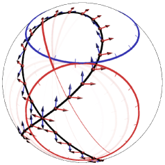
Figure 1. Minimal motion of the Viviani curve (rolling of spherical circles)

4. Discussion of results

This article unveiled some relations between rational motions and their trajectories. A rational curve occurs as trajectory of a unique (up to coordinate changes) rational motion of minimal degree in the dual quaternion model. This was a surprise to the authors as a mere trajectory seems to leave a lot of freedom for the construction of a suitable rational motion. Apparently, the requirement for minimality is rather restrictive.

Calling a rational curve “generic” if its circularity is zero and a rational motion “generic” if its primal part has no real factors (the spherical motion component has full degree), we may also say that rational motions of minimal quaternion degree to a generic trajectory are non-generic. Conversely, the trajectories of a generic rational motion are entirely circular and hence non generic.

In conjunction with the factorisation of generic rational motions [5] and its extension [8] to non-generic motion polynomials, our results contribute to a variant of Kempe’s Universality Theorem [3, Section 3.2] for rational space curves. Via motion factorisation, it is possible to construct linkages to generate a given rational motion and hence also a given rational trajectory. The dual quaternion degree of the generating motion is directly related to the number of links and joints in the mechanism. As a consequence, rational curves can be generated by spatial linkages with much fewer links and joints than those implied by the asymptotic bounds for algebraic space curves given by [1]. For circular curves, the numbers of links and joints are even less. A precise formulation and a rigorous proof will be worked out in a future paper.

Our main result in Corollary 2 raises questions. Is a similar uniqueness statement true for algebraic curves and algebraic motions? What rational motions are not minimal for any of their trajectories? The Darboux motion and the circular translation of Remark 1 are examples. Finally, determine simple (classes of) curves with simple minimal motion as in Example 3 and exploit their low degree and rationality in a CAGD or engineering context.

References

- [1] Timothy Good Abbott, Generalizations of Kempe’s universality theorem, Master’s thesis, Massachusetts Institute of Technology, 2008.
- [2] Oene Bottema and Bernhard Roth, Theoretical kinematics, Dover Publications, 1990.
- [3] Erik D. Demaine and Joseph O’Rourke, Geometric folding algorithms: Linkages, origami, polyhedra, Cambridge University Press, 2007.
- [4] Marco Hamann, Line-symmetric motions with respect to reguli, Mech. Machine Theory 46 (2011), no. 7, 960–974.
- [5] Gábor Hegedüs, Josef Schicho, and Hans-Peter Schröcker, Factorization of rational curves in the Study quadric and revolute linkages, Mech. Machine Theory 69 (2013), no. 1, 142–152.
- [6] B. Jüttler, Über zwangläufige rationale Bewegungsvorgänge, Sitzungsber. Österr. Akad. Wiss., Abt. II 202 (1993), 117–132.
- [7] Zijia Li, Josef Schicho, and Hans-Peter Schröcker, 7R Darboux linkages by factorization of motion polynomials, Accepted for publication in the Proceedings of the 14th IFToMM World Congress 2015, 2015, ArXiv cs.RO/1501.07365.
- [8] by same author, Factorization of motion polynomials, Submitted for publication, 2015, ArXiv cs.SC/1502.07600.
- [9] by same author, Spatial straight-line linkages by factorization of motion polynomials, Accepted for publication in ASME J. Mech. Robot., 2015, ArXiv math.MG/1410.2752.
- [10] Oystein Ore, Theory of non-commutative polynomials, Ann. of Math. (2) 34 (1933), no. 3, 480–508.
- [11] Martin Peternell, David Gruber, and Juana Sendra, Conchoid surfaces of spheres, Comput. Aided Geom. Design 30 (2013), no. 1, 35–44.
- [12] Jon Selig, Geometric fundamentals of robotics, 2 ed., Monographs in Computer Science, Springer, 2005.