Numerical computations of the dynamics of fluidic membranes and vesicles

Abstract

Vesicles and many biological membranes are made of two monolayers of lipid molecules and form closed lipid bilayers. The dynamical behaviour of vesicles is very complex and a variety of forms and shapes appear. Lipid bilayers can be considered as a surface fluid and hence the governing equations for the evolution include the surface (Navier–)Stokes equations, which in particular take the membrane viscosity into account. The evolution is driven by forces stemming from the curvature elasticity of the membrane. In addition, the surface fluid equations are coupled to bulk (Navier–)Stokes equations.

We introduce a parametric finite element method to solve this complex free boundary problem, and present the first three dimensional numerical computations based on the full (Navier–)Stokes system for several different scenarios. For example, the effects of the membrane viscosity, spontaneous curvature and area difference elasticity (ADE) are studied. In particular, it turns out, that even in the case of no viscosity contrast between the bulk fluids, the tank treading to tumbling transition can be obtained by increasing the membrane viscosity. Besides the classical tank treading and tumbling motions, another mode (called the transition mode in this paper, but originally called the vacillating-breathing mode and subsequently also called trembling, transition and swinging mode) separating these classical modes appears and is studied by us numerically. We also study how features of equilibrium shapes in the ADE and spontaneous curvature models, like budding behaviour or starfish forms, behave in a shear flow.

I Introduction

Lipid membranes consist of a bilayer of molecules, which have a hydrophilic head and two hydrophobic chains. These bilayers typically spontaneously form closed bag-like structures, which are called vesicles. It is observed that vesicles can attain a huge variety of shapes and some of them are similar to the biconcave shape of red blood cells. Since membranes play a fundamental role in many living systems, the study of vesicles is a very active research field in different scientific disciplines, see e.g. Seifert (1997); Baumgart et al. (2003); Noguchi and Gompper (2005a); McWhirter et al. (2009). It is the goal of this paper to present a numerical approach to study the evolution of lipid membranes. We present several computations showing quite different shapes, and the influence of fluid flow on the membrane evolution.

Since the classical papers of Canham (1970) and Helfrich (1973), there has been a lot of work with the aim of describing equilibrium membrane shapes with the help of elastic membrane energies. Canham (1970) and Helfrich (1973) introduced a bending energy for a non-flat membrane, which is formulated with the help of the curvature of the membrane. In the class of fixed topologies the relevant energy density, in the simplest situation, is proportional to the square of the mean curvature $\varkappa$. The resulting energy functional is called the Willmore energy. When computing equilibrium membrane shapes one has to take constraints into account. Lipid membranes have a very small compressibility, and hence can safely be modelled as locally incompressible. In addition, the presence of certain molecules in the surrounding fluid, for which the membrane is impermeable, leads to an osmotic pressure, which results in a constraint for the volume enclosed by the membrane. The minimal energetic model for lipid membranes consists of the Willmore mean curvature functional together with enclosed volume and surface area constraints. Already this simple model leads to quite different shapes including the biconcave red blood cell shapes, see Seifert (1997).

Helfrich (1973) introduced a variant of the Willmore energy, with the aim of modelling a possible asymmetry of the bilayer membrane. Helfrich (1973) studied the functional $\int(\varkappa-\overline{\varkappa})^{2}$, where $\overline{\varkappa}$ is a fixed constant, the so-called spontaneous curvature. It is argued that the origin of the spontaneous curvature is e.g. a different chemical environment on both sides of the membrane. We refer to Martens and McMahon (2008) and Kamal et al. (2009) for a recent discussion, and for experiments in situations which lead to spontaneous curvature effects due to the chemical structure of the bilayer.

Typically there is yet another asymmetry in the bilayer leading to a signature in the membrane architecture. This results from the fact that the two membrane layers have a different number of molecules. Since the exchange of molecules between the layers is difficult, an imbalance is conserved during a possible shape change. The total area difference between the two layers is proportional to $M=\int\varkappa$. Several models have been proposed, which describe the difference in the total number of molecules in the two layers with the help of the integrated mean curvature. The bilayer coupling model, introduced by Svetina and coworkers Svetina et al. (1982); Svetina and Zeks (1983, 1989), assumes that the area per lipid molecule is fixed and assumes that there is no exchange of molecules between the two layers. Hence the total areas of the two layers are fixed, and on assuming that the two layers are separated by a fixed distance, one obtains, to the order of this distance, that the area difference can be approximated by the integrated mean curvature, see Svetina et al. (1982); Svetina and Zeks (1983, 1989). We note that a spontaneous curvature contribution is irrelevant in the bilayer coupling model as this would only add a constant to the energy as the area and integrated mean curvature are fixed.

Miao et al. (1994) noted that in the bilayer coupling model budding always occurs continuously which is inconsistent with experiments. They hence studied a model in which the area of the two layers are not fixed but can expand or compress under stress. Given a relaxed initial area difference $\Delta A_{0}$, the total area difference $\Delta A$, which is proportional to the integrated mean curvature, can deviate from $\Delta A_{0}$. However, the total energy now has a contribution that is proportional to $(\Delta A-\Delta A_{0})^{2}$. This term describes the elastic area difference stretching energy, see Miao et al. (1994); Seifert (1997), and hence one has to pay a price energetically to deviate from the relaxed area difference.

It is also possible to combine the area difference elasticity model (ADE-model) with a spontaneous curvature assumption, see Miao et al. (1994) and Seifert (1997). However, the resulting energetical model is equivalent to an area difference elasticity model with a modified $\Delta A_{0}$, see Seifert (1997) for a more detailed discussion.

It has been shown that the bilayer coupling model (BC-model) and the area difference elasticity model (ADE-model) lead to a multitude of shapes, which also have been observed in experiments with vesicles. Beside others, the familiar discocyte shapes (including the “shape” of a red blood cell), stomatocyte shapes, prolate shapes and pear-like shapes have been observed. In addition, the budding of membranes can be described, as well as more exotic shapes, like starfish vesicles. Moreover, higher genus shapes appear as global or local minima of the energies discussed above. We refer to Seifert (1997); Ziherl and Svetina (2005); Miao et al. (1994); Seifert et al. (1991); Wintz et al. (1996) for more details on the possible shapes appearing, when minimizing the energies in the ADE- and BC-models.

Configurational changes of vesicles and membranes cannot be described by energetical considerations alone, but have to be modelled with the help of appropriate evolution laws. Several authors considered an $L^{2}$–gradient flow dynamics of the curvature energies discussed above. Pure Willmore flow has been studied in Mayer and Simonett (2002); Clarenz et al. (2004); Dziuk (2008); Barrett et al. (2008); Du et al. (2005); Franken et al. (2013), where the last two papers use a phase field formulation of the Willmore problem. Some authors also took other aspects, such as constraints on volume and area Barrett et al. (2008); Bonito et al. (2010); Du et al. (2004), as well as a constraint on the integrated mean curvature Barrett et al. (2008); Du et al. (2005), into account. The effect of different lipid components in an $L^{2}$–gradient flow approach of the curvature energy has been studied in Elliott and Stinner (2010); Bartels et al. (2012); Mercker et al. (2013); Du et al. (2009); Boedec et al. (2011); Rahimi and Arroyo (2012); Rodrigues et al. (2015).

The above mentioned works considered a global constraint on the surface area. The membrane, however, is locally incompressible and hence a local constraint on the evolution of the membrane molecules should be taken into account. Several authors included the local inextensibility constraint by introducing an inhomogeneous Lagrange multiplier for this constraint on the membrane. This approach has been used within the context of different modelling and computational strategies such as the level set approach Salac and Miksis (2011, 2012); Laadhari et al. (2014); Doyeux et al. (2013), the phase field approach Biben et al. (2005); Jamet and Misbah (2007); Aland et al. (2014), the immersed boundary method Kim and Lai (2010, 2012); Hu et al. (2014), the interfacial spectral boundary element method Dodson and Dimitrakopoulos (2011) and the boundary integral method Farutin et al. (2014).

The physically most natural way to consider the local incompressibility constraint makes use of the fact that the membrane itself can be considered as an incompressible surface fluid. This implies that a surface Navier–Stokes system has to be solved on the membrane. The resulting set of equations has to take forces stemming from the surrounding fluid and from the membrane elasticity into account. In total, bulk Navier–Stokes equations coupled to surface Navier–Stokes equations have to be solved. As the involved Reynolds numbers for vesicles are typically small one can often replace the full Navier–Stokes equations by the Stokes systems on the surface and in the bulk. The incompressibility condition in the bulk (Navier–)Stokes equations naturally leads to conservation of the volume enclosed by the membrane and the incompressibility condition on the surface leads a conservation of the membrane’s surface area. A model involving coupled bulk-surface (Navier–)Stokes equations has been proposed by Arroyo and DeSimone (2009), and it is this model that we want to study numerically in this paper.

Introducing forces resulting from membrane energies in fluid flow models has been studied numerically before by different authors, Salac and Miksis (2011, 2012); Laadhari et al. (2014); Jamet and Misbah (2007); Aland et al. (2014); Hu et al. (2014). However, typically these authors studied simplified models, and either volume or surface constraints were enforced by Lagrange multipliers. In addition, either just the bulk or just the surface (Navier–)Stokes equations have been solved. The only work considering simultaneously bulk and surface Navier–Stokes equations are Arroyo et al. (2010) and Barrett et al. (2014, 2015a), where the former work is restricted to axisymmetric situations. In the present paper we are going to make use of the numerical method introduced in Barrett et al. (2015a), see also Barrett et al. (2014).

The paper is organized as follows. In the next section we precisely state the mathematical model, consisting of the curvature elasticity model together with a coupled bulk-surface (Navier–)Stokes system. In Section III we introduce our numerical method which consists of an unfitted parametric finite element method for the membrane evolution. The curvature forcing is discretized and coupled to the Navier–Stokes system in a stable way using the finite element method for the fluid unknowns. Numerical computations in Section IV demonstrate that we can deal with a variety of different membrane shapes and flow scenarios. In particular, we will study what influence the membrane viscosity, the area difference elasticity (ADE) and the spontaneous curvature have on the evolution of bilayer membranes in shear flow. We finish with some conclusions.

II A continuum model for fluidic membranes

We consider a continuum model for the evolution of biomembranes and vesicles, which consists of a curvature elasticity model for the membrane and the Navier–Stokes equations in the bulk and on the surface. The model is based on a paper by Arroyo and DeSimone (2009), where in addition we also allow the curvature energy model to be an area difference elasticity model. We first introduce the curvature elasticity model and then describe the coupling to the surface and bulk Navier–Stokes equations.

The thickness of the lipid bilayer in a vesicle is typically three to four orders of magnitude smaller than the typical size of the vesicle. Hence the membrane can be modelled as a two dimensional surface $\Gamma$ in $\mathbb{R}^{3}$. Given the principal curvatures $\varkappa_{1}$ and $\varkappa_{2}$ of $\Gamma$, one can define the mean curvature

$$\varkappa=\varkappa_{1}+\varkappa_{2}$$

and the Gauß curvature

$$K=\varkappa_{1}\,\varkappa_{2}$$

(as often in differential geometry we choose to take the sum of the principal curvatures as the mean curvature, instead of its mean value). The classical works of Canham (1970) and Helfrich (1973) derive a local bending energy, with the help of an expansion in the curvature, and they obtain

$$\int_{\Gamma}\left(\frac{\alpha}{2}\,\varkappa^{2}+\alpha_{G}\,K\right)\;{\rm d}s$$ (1)

as the total energy of a symmetric membrane. The parameters $\alpha,\alpha_{G}$ have the dimension of energy and are called the bending rigidity $\alpha$ and the Gaussian bending rigidity $\alpha_{G}$. If we consider closed membranes with a fixed topology, the term $\int_{\Gamma}K\;{\rm d}s$ is constant and hence we will neglect the Gaussian curvature term in what follows.

As discussed above, the total area difference $\Delta A$ of the two lipid layers is, to first order, proportional to

$$M(\Gamma)=\int_{\Gamma}\varkappa\;{\rm d}s\,.$$

Taking now into account that there is an optimal area difference $\Delta A_{0}$, the authors in Seifert et al. (1992); Wiese et al. (1992); Bozic et al. (1992) added a term proportional to

$$(M(\Gamma)-M_{0})^{2}$$

to the curvature energy, where $M_{0}$ is a fixed constant which is proportional to the optimal area difference.

For non-symmetric membranes a certain mean curvature $\overline{\varkappa}$ can be energetically favourable. Then the elasticity energy (1) is modified to

$$\int_{\Gamma}\left(\frac{\alpha}{2}\,(\varkappa-\overline{\varkappa})^{2}+\alpha_{G}\,K\right)\;{\rm d}s\,.$$

The constant $\overline{\varkappa}$ is called spontaneous curvature. Taking into account that $\int_{\Gamma}\alpha_{G}\,K\;{\rm d}s$ does not change for an evolution within a fixed topology class, the most general bending energy that we use in this paper is given by $\alpha\,E(\Gamma)$ with the dimensionless energy

$$E(\Gamma)=\frac{1}{2}\,\int_{\Gamma}(\varkappa-\overline{\varkappa})^{2}\;{\rm d}s+\frac{\beta}{2}\,(M(\Gamma)-M_{0})^{2}\,,$$ (2)

where $\beta$ has the dimension $(\frac{1}{{\rm length}})^{2}$.

We now consider a continuum model for the fluid flow on the membrane and in the bulk, inside and outside of the membrane. We assume that the closed, time dependent membrane $(\Gamma(t))_{t\geq 0}$ lies inside a spatial domain $\Omega\subset\mathbb{R}^{3}$. For all times the membrane separates $\Omega$ into an inner domain $\Omega_{-}(t)$ and an outer domain $\Omega_{+}(t)$. Denoting by $\vec{u}$ the fluid velocity and by $p$ the pressure, the bulk stress tensor is given by $\underline{\underline{\sigma}}\rule{0.0pt}{0.0pt}=2\,\mu\,\underline{\underline{D}}\rule{0.0pt}{0.0pt}(\vec{u})-p\,\underline{\underline{\rm Id}}\rule{0.0pt}{0.0pt}$, with $\underline{\underline{D}}\rule{0.0pt}{0.0pt}(\vec{u})=\tfrac{1}{2}\,(\nabla\,\vec{u}+(\nabla\,\vec{u})^{T})$ being the bulk rate-of-strain tensor. We assume that the Navier–Stokes system

$$\rho\,(\vec{u}_{t}+(\vec{u}\,.\,\nabla)\,\vec{u})-\nabla\,.\,\underline{\underline{\sigma}}\rule{0.0pt}{0.0pt}=0\,,\quad\nabla\,.\,\vec{u}=0$$

holds in $\Omega_{-}(t)$ and $\Omega_{+}(t)$. Here $\rho$ and $\mu$ are the density and dynamic viscosity of the fluid, which can take different (constant) values $\rho_{\pm}$, $\mu_{\pm}$ in $\Omega_{\pm}(t)$. Arroyo and DeSimone (2009) used the theory of interfacial fluid dynamics, which goes back to Scriven (1960), to introduce a relaxation dynamics for fluidic membranes. In this model the fluid velocity is assumed to be continuous across the membrane, the membrane is moved in the normal direction with the normal velocity of the bulk fluid and, in addition, the surface Navier–Stokes equations

$$\rho_{\Gamma}\,\partial_{t}^{\bullet}\,\vec{u}-\nabla_{\!s}\,.\,\underline{\underline{\sigma}}\rule{0.0pt}{0.0pt}_{\Gamma}=[\underline{\underline{\sigma}}\rule{0.0pt}{0.0pt}]^{+}_{-}\,\vec{\nu}+\alpha\,\vec{f}_{\Gamma}\,,\quad\nabla_{\!s}\,.\,\vec{u}=0$$

have to hold on $\Gamma(t)$. Here $\rho_{\Gamma}$ is the surface material density, $\partial_{t}^{\bullet}$ is the material derivative and $\nabla_{\!s},\nabla_{\!s}\,.$ are the gradient and divergence operators on the surface. The surface stress tensor is given by

$$\underline{\underline{\sigma}}\rule{0.0pt}{0.0pt}_{\Gamma}=2\,\mu_{\Gamma}\,\underline{\underline{D}}\rule{0.0pt}{0.0pt}_{s}(\vec{u})-p_{\Gamma}\,\underline{\underline{\mathcal{P}}}\rule{0.0pt}{0.0pt}_{\Gamma}\,,$$

where $p_{\Gamma}$ is the surface pressure, $\mu_{\Gamma}$ is the surface shear viscosity, $\underline{\underline{\mathcal{P}}}\rule{0.0pt}{0.0pt}_{\Gamma}$ is the projection onto the tangent space and

$$\underline{\underline{\mathcal{D}}}\rule{0.0pt}{0.0pt}_{s}(\vec{u})=\tfrac{1}{2}\,\underline{\underline{\mathcal{P}}}\rule{0.0pt}{0.0pt}_{\Gamma}\,(\nabla_{\!s}\,\vec{u}+(\nabla_{\!s}\,\vec{u})^{T})\,\underline{\underline{\mathcal{P}}}\rule{0.0pt}{0.0pt}_{\Gamma}$$

is the surface rate-of-strain tensor. Furthermore, the term $[\underline{\underline{\sigma}}\rule{0.0pt}{0.0pt}]^{+}_{-}\,\vec{\nu}=\underline{\underline{\sigma}}\rule{0.0pt}{0.0pt}_{+}\,\vec{\nu}-\underline{\underline{\sigma}}\rule{0.0pt}{0.0pt}_{-}\,\vec{\nu}$ is the force exerted by the bulk on the membrane, where $\vec{\nu}$ denotes the exterior unit normal to $\Omega_{-}(t)$. The remaining term $\alpha\,\vec{f}_{\Gamma}$ denotes the forces stemming from the elastic bending energy. These forces are given by the first variation of the bending energy $\alpha\,E(\Gamma(t))$, see Seifert (1997); Arroyo and DeSimone (2009). It turns out that $\vec{f}_{\Gamma}$ points in the normal direction, i.e. $\vec{f}_{\Gamma}=f_{\Gamma}\,\vec{\nu}$, and we obtain, see Willmore (1965); Seifert (1997),

$$f_{\Gamma} =-\Delta_{s}\,\varkappa-(\varkappa-\overline{\varkappa})\,|\nabla_{\!s}\,\vec{\nu}|^{2}+\tfrac{1}{2}\,(\varkappa-\overline{\varkappa})^{2}\,\varkappa$$

$$\quad+\beta\,(M(\Gamma)-M_{0})\,(|\nabla_{\!s}\,\vec{\nu}|^{2}-\varkappa^{2})\quad\text{on }\Gamma(t)\,.$$

Here $\Delta_{s}$ is the surface Laplace operator, $\nabla_{\!s}\,\vec{\nu}$ is the Weingarten map and $|\nabla_{\!s}\,\vec{\nu}|^{2}=\varkappa^{2}_{1}+\varkappa^{2}_{2}$. Assuming e.g. no-slip boundary conditions on $\partial\Omega$, the boundary of $\Omega$, we obtain that the total energy can only decrease, i.e.

$$\frac{\rm d}{{\rm d}t}\left(\int_{\Omega}\frac{\rho}{2}\,|\vec{u}|^{2}\;{\rm d}x+\frac{\rho_{\Gamma}}{2}\,\int_{\Gamma}|\vec{u}|^{2}\;{\rm d}s+\alpha\,E(\Gamma)\right)$$

$$\,=-2\left(\int_{\Omega}\mu\,|\underline{\underline{D}}\rule{0.0pt}{0.0pt}(\vec{u})|^{2}\;{\rm d}x+\mu_{\Gamma}\int_{\Gamma}|\underline{\underline{D}}\rule{0.0pt}{0.0pt}_{s}(\vec{u})|^{2}\;{\rm d}s\right)\leq 0\,.$$ (3)

We now non-dimensionalize the problem. We choose a time scale $\tilde{t}$, a length scale $\tilde{x}$ and the resulting velocity scale $\tilde{u}=\tilde{x}/\tilde{t}$. Then we define the bulk and surface Reynolds numbers

$${\rm Re}={\tilde{x}\,\rho_{+}\,\tilde{u}}/{\mu_{+}}\quad\text{and}\quad{\rm Re}_{\Gamma}={\tilde{x}\,\rho_{\Gamma}\,\tilde{u}}/{\mu_{\Gamma}}\,,$$

the bulk and surface pressure scales

$$\tilde{p}={\mu_{+}}/{\tilde{t}}\quad\text{and}\quad\tilde{p}_{\Gamma}={\mu_{+}\,\tilde{x}}/{\tilde{t}}=\mu_{+}\,\tilde{u}\,,$$

and

$$\rho^{*} =\rho/\rho_{+}=\begin{cases}1&\text{in $\Omega_{+}$}\\ \rho_{-}/\rho_{+}&\text{in $\Omega_{-}$}\end{cases}\,,$$

$$\mu^{*} =\mu/\mu_{+}=\begin{cases}1&\text{in $\Omega_{+}$}\\ \Lambda&\text{in $\Omega_{-}$}\end{cases}\,,\quad\Lambda=\mu_{-}/\mu_{+}\,,$$

$$\mu_{\Gamma}^{*} ={\mu_{\Gamma}}/({\mu_{+}\,\tilde{x}})\,,$$

as well as the new independent variables $\widehat{x}=x/\tilde{x}$, $\widehat{t}=t/\tilde{t}$. For the unknowns

$$\vec{\widehat{u}}={\vec{u}}/{\tilde{u}}\,\,,\,\,\widehat{p}={p}/{\tilde{p}}\,\,,\,\,\widehat{p}_{\Gamma}={p_{\Gamma}}/{\tilde{p}_{\Gamma}}$$

we now obtain the following set of equations (on dropping the $\widehat{\phantom{u}}$-notation for the new variables for ease of exposition)

$${\rm Re}\,\rho^{*}\,(\vec{u}_{t}+(\vec{u}\,.\,\nabla)\,\vec{u})-\mu^{*}\,\Delta\,\vec{u}+\nabla\,p=0\quad\text{in }\Omega_{\pm}(t)\,,$$

$${\rm Re}_{\Gamma}\,\mu_{\Gamma}^{*}\,\partial_{t}^{\bullet}\,\vec{u}-\nabla_{\!s}\,.\left(2\,\mu_{\Gamma}^{*}\,\underline{\underline{D}}\rule{0.0pt}{0.0pt}_{s}(\vec{u})-p_{\Gamma}\,\underline{\underline{\mathcal{P}}}\rule{0.0pt}{0.0pt}_{\Gamma}\right)$$

$$\hskip 17.07164pt=\left[2\,\mu^{*}\,\underline{\underline{D}}\rule{0.0pt}{0.0pt}(\vec{u})-p\,\underline{\underline{\rm Id}}\rule{0.0pt}{0.0pt}\right]^{+}_{-}\vec{\nu}+\alpha^{*}\,{\vec{f}^{*}_{\Gamma}}\quad\text{on }\Gamma(t)\,,$$ (4)

with $\vec{f}^{*}_{\Gamma}=f^{*}_{\Gamma}\,\vec{\nu}$,

$$f^{*}_{\Gamma} =-\Delta_{s}\,\varkappa-(\varkappa-\overline{\varkappa}^{*})\,|\nabla_{\!s}\,\vec{\nu}|^{2}+\tfrac{1}{2}\,(\varkappa-\overline{\varkappa}^{*})^{2}\,\varkappa$$

$$\qquad+\beta^{*}\,(M(\Gamma)-M^{*}_{0})\,(|\nabla_{\!s}\,\vec{\nu}|^{2}-\varkappa^{2})\quad\text{on }\Gamma(t)\,,$$ (5)

$\alpha^{*}={\alpha}/{(\mu_{+}\,\tilde{u}\,\tilde{x}^{2})}$ and $\overline{\varkappa}^{*}=\tilde{x}\,\overline{\varkappa}$, $M^{*}_{0}=M_{0}/\tilde{x}$, $\beta^{*}=\tilde{x}^{2}\,\beta$. We remark that the Reynolds numbers for the two regions in the bulk are given by ${\rm Re}$ and ${\rm Re}\,\rho^{*}/\mu^{*}$, respectively, and that they will in general differ in the case of a viscosity contrast between the inner and outer fluid. In addition to the above equations, we of course also require that $\vec{u}$ has zero divergence in the bulk and that the surface divergence of $\vec{u}$ vanishes on $\Gamma$.

Typical values for the bulk dynamic viscosity $\mu$ are around $10^{-3}-10^{-2}\frac{\rm kg}{\rm s\,m}$, see Arroyo and DeSimone (2009); McWhirter et al. (2009); Faivre (2006), whereas the surface shear viscosity typically is about $10^{-9}-10^{-8}\frac{\rm kg}{\rm s}$, see Abreu et al. (2014); McWhirter et al. (2009); Rodrigues et al. (2015). The bending modulus $\alpha$ is typically $10^{-20}-10^{-19}\frac{\rm kg\,m^{2}}{\rm s^{2}}$, see Faivre (2006); Abreu et al. (2014); Rodrigues et al. (2015).

The term $\mu_{\Gamma}^{*}=\mu_{\Gamma}/({\mu_{+}\,\tilde{x}})$ in (II) suggests to choose the length scale

$$\tilde{x}={\mu_{\Gamma}}/{\mu_{+}}\quad\iff\quad\mu_{\Gamma}^{*}=1\,.$$

As $\alpha^{*}={\alpha}/{(\mu_{+}\,\tilde{u}\,\tilde{x}^{2})}={\alpha\,\tilde{t}}/{(\mu_{+}\,\tilde{x}^{3})}$ appears in (II), we choose the time scale

$$\tilde{t}={\mu_{+}\,\tilde{x}^{3}}/{\alpha}\,.$$

Choosing

$$\mu_{\Gamma}=5\cdot 10^{-9}\frac{\rm kg}{\rm s}\,\,,\,\,\mu_{+}=10^{-3}\frac{\rm kg}{\rm s\,m}\,\,,\,\,\alpha=10^{-19}\frac{\rm kg\,m^{2}}{\rm s^{2}}\,,$$

see e.g. Arroyo and DeSimone (2009), we obtain the length scale $5\cdot 10^{-6}\rm m$ and the time scale $1.25\rm s$, which are typical scales in experiments. With these scales for length and time together with values of $\sim 10^{3}\rm kg/m^{3}$ for the bulk density and $\sim 10^{-6}\rm kg/m^{2}$ for the surface densities, we obtain for the bulk and surface Reynolds numbers

$${\rm Re}\approx 10^{-5}\quad\text{and}\quad{\rm Re}_{\Gamma}\approx 10^{-8}\,,$$

and hence we will set the Reynolds numbers to zero in this paper. We note that it is straightforward to also consider positive Reynolds numbers in our numerical algorithm, see Barrett et al. (2014, 2015a) for details. Together with the other observations above, we then obtain the following reduced set of equations.

$$-\mu^{*}\,\Delta\,\vec{u}+\nabla\,p=0\quad\text{in }\Omega_{\pm}(t)\,,$$

$$-2\,\nabla_{\!s}\,.\,\underline{\underline{D}}\rule{0.0pt}{0.0pt}_{s}(\vec{u})+\nabla_{\!s}\,.\,(p_{\Gamma}\,\underline{\underline{\mathcal{P}}}\rule{0.0pt}{0.0pt}_{\Gamma})$$

$$\hskip 36.98866pt=\left[2\,\mu^{*}\,\underline{\underline{D}}\rule{0.0pt}{0.0pt}(\vec{u})-p\,\underline{\underline{\rm Id}}\rule{0.0pt}{0.0pt}\right]^{+}_{-}\vec{\nu}+\alpha^{*}\,\vec{f}_{\Gamma}^{*}\quad\text{on }\Gamma(t)\,.$$ (6)

A downside of the scaling used to obtain (II) is that the surface viscosity no longer appears as an independent parameter. However, studying the effect of the surface viscosity, e.g. on the tank treading to tumbling transition in shearing experiments, is one of the main focuses of this paper. It is for this reason that we also consider the following alternative scaling, when suitable length and velocity scales are at hand. For example, we may choose the length scale $\tilde{x}$ based on the (fixed) size of the membrane and a velocity scale $\tilde{u}$ based on appropriate boundary velocity values. In this case we obtain from (II), for small Reynolds numbers, the following set of equations

$$-\mu^{*}\,\Delta\,\vec{u}+\nabla\,p=0\quad\text{in }\Omega_{\pm}(t)\,,$$

$$-\nabla_{\!s}\,.\left(2\,\mu_{\Gamma}^{*}\,\underline{\underline{D}}\rule{0.0pt}{0.0pt}_{s}(\vec{u})-p_{\Gamma}\,\underline{\underline{\mathcal{P}}}\rule{0.0pt}{0.0pt}_{\Gamma}\right)$$

$$\hskip 36.98866pt=\left[2\,\mu^{*}\,\underline{\underline{D}}\rule{0.0pt}{0.0pt}(\vec{u})-p\,\underline{\underline{\rm Id}}\rule{0.0pt}{0.0pt}\right]^{+}_{-}\vec{\nu}+\alpha^{*}\,\vec{f}_{\Gamma}^{*}\quad\text{on }\Gamma(t)\,.$$ (7)

Note that here three non-dimensional parameters remain: $\mu_{\Gamma}^{*}$, $\Lambda$ and $\alpha^{*}$. Here $\mu_{\Gamma}^{*}$ compares the surface shear viscosity to the bulk shear viscosity, $\Lambda$ is the bulk viscosity ratio and $\alpha^{*}$ is an inverse capillary number, which describes the ratio of characteristic membrane stresses to viscous stresses. Clearly, the system (II) corresponds to (II) with $\mu_{\Gamma}^{*}=1$. Hence from now on, we will only consider the scaling (II) in detail.

Of course, the system (II) needs to be supplemented with a boundary condition for $\vec{u}$ or $\underline{\underline{\sigma}}\rule{0.0pt}{0.0pt}$, and with an initial condition for $\Gamma(0)$. For the former we partition the boundary $\partial\Omega$ of $\Omega$ into $\partial_{1}\Omega$, where we prescribe a fixed velocity $\vec{u}=\vec{g}$, and $\partial_{2}\Omega$, where we prescribe the stress-free condition $\underline{\underline{\sigma}}\rule{0.0pt}{0.0pt}\,\vec{\rm n}=\vec{0}$, with $\vec{\rm n}$ denoting the outer normal to $\Omega$.

We note that our non-dimensionalization may be different to others presented in the literature. Often the length scale $a=(\frac{\mathcal{A}(0)}{4\,\pi})^{\frac{1}{2}}$ is chosen, where $\mathcal{A}(0)$ denotes the surface area of the vesicle at time zero, see e.g. Spann et al. (2014). Our length scale $\tilde{x}$ may lead to simulations with $\mathcal{A}(0)=4\,\pi\,S^{2}$, with $S>0$, so that our non-dimensional parameters in (II) correspond to the non-dimensional values for a fixed length scale $\tilde{x}=a$ as follows:

$$\mathcal{M}=\frac{\mu_{\Gamma}}{\mu_{+}\,a}=\frac{\mu_{\Gamma}^{*}}{S}\,,\ a\,\overline{\varkappa}=S\,\overline{\varkappa}^{*}\,,\ {\rm Ca}=\frac{\mu_{+}\,\tilde{u}\,a^{3}}{\tilde{x}\,\alpha}=\frac{S^{3}}{\alpha^{*}}\,.$$ (8)

III Numerical approximation

The numerical computations in this paper have been performed with a finite element approximation introduced by the authors in Barrett et al. (2015a). The approach discretizes the bulk and surface degrees of freedom independently. In particular, the surface mesh is not a restriction of the bulk mesh. The bulk degrees of freedoms $\vec{u}$ and $p$ are discretized with the lowest order Taylor–Hood element, P2–P1, in our numerical computations. The evolution of the membrane is tracked with the help of parametric meshes $\Gamma^{h}$, which are updated by the fluid velocity. Since the membrane surface is locally incompressible, it turns out that the surface mesh has good mesh properties during the evolution. This is in contrast to other fluid problems with interfaces in which the mesh often deteriorates during the evolution when updated with the fluid velocity, see e.g. Bänsch (2001).

The non-dimensionalized elastic forcing by the membrane curvature energy, $\vec{f}_{\Gamma}^{*}$ in (II), is discretized with the help of a weak formulation by Dziuk (2008), which is generalized by Barrett et al. (2015a) to take spontaneous curvature and area difference elasticity effects into account. A main ingredient of the numerical approach is the fact that one can use a weak formulation of (II) that can be discretized in a stable way. In fact, defining $A^{*}=\beta^{*}\,(M(\Gamma)-M_{0}^{*})$ and $\vec{y}=\vec{\varkappa}+(A^{*}-\overline{\varkappa}^{*})\,\vec{\nu}$ the following identity, which has to hold for all $\vec{\chi}$ on $\Gamma$, characterizes $\vec{f}_{\Gamma}^{*}$:

$$\left\langle\vec{f}_{\Gamma}^{*},\vec{\chi}\right\rangle=\left\langle\nabla_{\!s}\,\vec{y},\nabla_{\!s}\,\vec{\chi}\right\rangle+\left\langle\nabla_{\!s}\,.\,\vec{y},\nabla_{\!s}\,.\,\vec{\chi}\right\rangle$$

$$\ -2\left\langle(\nabla_{\!s}\,\vec{y})^{T},\underline{\underline{D}}\rule{0.0pt}{0.0pt}_{s}(\vec{\chi})\,(\nabla_{\!s}\,\vec{\rm}id)^{T}\right\rangle+(A^{*}-\overline{\varkappa}^{*})\left\langle\vec{\varkappa},[\nabla_{\!s}\,\vec{\chi}]^{T}\,\vec{\nu}\right\rangle$$

$$\ -\tfrac{1}{2}\left\langle[|\vec{\varkappa}-\overline{\varkappa}^{*}\,\vec{\nu}|^{2}-2\,(\vec{y}\,.\,\vec{\varkappa})]\,\nabla_{\!s}\,\vec{\rm}id,\nabla_{\!s}\,\vec{\chi}\right\rangle$$

$$\ -A^{*}\left\langle(\vec{\varkappa}\,.\,\vec{\nu})\,\nabla_{\!s}\,\vec{\rm}id,\nabla_{\!s}\,\vec{\chi}\right\rangle.$$

Here $\langle\cdot,\cdot\rangle$ is the $L^{2}$–inner product on $\Gamma$, and $\nabla_{\!s}\,\vec{y}=\left(\partial_{s_{j}}\,y_{i}\right)_{i,j=1}^{3}$ with $(\partial_{s_{1}},\partial_{s_{2}},\partial_{s_{3}})^{T}=\nabla_{\!s}$. Roughly speaking the above identity shows that $\vec{f}_{\Gamma}^{*}$ has a divergence structure. We remark here that similar divergence structures have been derived with the help of Noether’s theorem, see Capovilla and Guven (2004); Lengeler (2015).

The numerical method of Barrett et al. (2015a) has the feature that a semi-discrete, i.e. continuous in time and discrete in space, version of the method obeys a discrete analog of the energy inequality (3). In addition, this semi-discrete version has the property that the volume enclosed by the vesicle and the membrane’s surface area are conserved exactly. After discretization in time these properties are approximately fulfilled to a high accuracy, see Section IV. The fully discrete system is linear and fully coupled in the unknowns. The overall system is reduced by a Schur complement approach to obtain a reduced system in just velocity and pressure unknowns. For this resulting linear system well-known solution techniques for finite element discretizations for the standard Navier–Stokes equations can be used, see Barrett et al. (2015b).

IV Numerical computations

In shearing experiments the inclination angle of the vesicle in the shear flow direction is often of interest. Here we will always consider shear flow in the $x_{1}$ direction with $x_{3}$ being the flow gradient direction. Precisely, if $\overline{\Omega}=[-L,L]^{2}\times[-W,W]$, then we prescribe the inhomogeneous Dirichlet boundary condition $\vec{g}(\vec{x})=(x_{3},0,0)^{T}$ on the top and bottom boundaries $\partial_{1}\Omega=[-L,L]^{2}\times\{\pm W\}$. Assuming the vesicle’s centre of mass is at the origin, then $\underline{\underline{{\rm M}}}\rule{0.0pt}{0.0pt}=\int_{\Omega_{-}(t)}|\vec{x}|^{2}\,\underline{\underline{\rm Id}}\rule{0.0pt}{0.0pt}-\vec{x}\otimes\vec{x}\;{\rm d}x$ denote the vesicle’s moment of inertia tensor. Let $\vec{p}$, with $|\vec{p}|=1$ and $p_{1}\geq 0$, be the eigenvector corresponding to the smallest eigenvalue of $\underline{\underline{{\rm M}}}\rule{0.0pt}{0.0pt}$. Then the vesicle’s inclination angle is defined by $\theta=\arg(p_{1}+{\rm i}\,p_{3})\in(-\pi/2,\pi/2]$, where $\arg:\mathbb{C}\to(-\pi,\pi]$. For later use we also note that the deformation parameter $D$ is defined by $(b-c)/(b+c)$, where $b,c$ are the major and minor semiaxes of an ellipsoid with the same moment of inertia tensor, see e.g. Ramanujan and Pozrikidis (1998). Hence, in 2d, $D=(\lambda_{\max}^{\frac{1}{2}}-\lambda_{\min}^{\frac{1}{2}})/(\lambda_{\max}^{\frac{1}{2}}+\lambda_{\min}^{\frac{1}{2}})$, where $\lambda_{\max}$ and $\lambda_{\min}$ are the two eigenvalues of $\underline{\underline{{\rm M}}}\rule{0.0pt}{0.0pt}$.

The inclination angle $\theta$ is important for the classification of different types of dynamics in the shear flow experiments that we will present. The classical deformation dynamics for vesicles are the tank treading (TT) and the tumbling (TU) motions. In the tank treading motion the vesicle adopts a constant inclination angle in the flow, while the surface fluid rotates on the membrane surface. This motion is observed for small viscosity contrasts between the inner and the outer fluid and, as we will see later, at low surface membrane viscosity. At large viscosity contrasts or large membrane viscosity the tumbling motion occurs. In the tumbling regime the membrane rotates as a whole, and the inclination angle oscillates in the whole interval $(-\pi/2,\pi/2]$. In the last ten years a new dynamic regime for vesicles in shear flow has been identified. In this regime the inclination angle is neither constant nor does it oscillate in the whole interval $(-\pi/2,\pi/2]$. The dynamics are characterized by periodic oscillations of the inclination angle $\theta$ such that $\theta\in[-\theta_{0},\theta_{0}]$ for a $\theta_{0}$ in the open interval $(0,\pi/2)$. This regime was first predicted theoretically by Misbah (2006) and subsequently observed experimentally in Kantsler and Steinberg (2006). Later this regime has been studied by different groups, see e.g. Zabusky et al. (2011); Noguchi and Gompper (2007); Yazdani and Bagchi (2012); Farutin and Misbah (2012); Abreu et al. (2014); Biben et al. (2011); Spann et al. (2014) for more details. In Misbah (2006) this motion was called vacillating-breathing and later the same motion was also called trembling, transition mode or swinging. Following Yazdani and Bagchi (2012) we will refer to this new regime as the transition (TR) mode.

In our numerical simulations we will only consider the scaling (II). For all the presented simulations we will state the reduced volume as a characteristic invariant. It is defined as $\mathcal{V}_{r}=6\,\pi^{\frac{1}{2}}\,\mathcal{V}(0)/\mathcal{A}^{\frac{3}{2}}(0)$, see e.g. Wintz et al. (1996). Here $\mathcal{V}(t)$ and $\mathcal{A}(t)$ denote the volume of the discrete inner phase and the discrete surface area, respectively, at time $t$. Moreover, if nothing else is specified, then our numerical simulations are for no-slip boundary conditions, i.e. $\partial_{1}\Omega=\partial\Omega$ and $\vec{g}=\vec{0}$. In all our experiments it holds that $\overline{\varkappa}^{*}\,\beta^{*}=0$, and we will only report the values of $\overline{\varkappa}^{*}$ and $\beta^{*}$ for simulations where they are nonzero. Here we recall, as stated in the introduction, that the energy

$$E^{*}(\Gamma)=\frac{1}{2}\,\int_{\Gamma}(\varkappa-\overline{\varkappa}^{*})^{2}\;{\rm d}s+\frac{\beta^{*}}{2}\,(M(\Gamma)-M^{*}_{0})^{2}$$ (9)

for $\overline{\varkappa}^{*}\,\beta^{*}\not=0$ is equivalent to (9) with $\overline{\varkappa}^{*}=0$, the same value of $\beta^{*}>0$, and a modified value of $M_{0}^{*}$. Finally, we stress that our sign convention for curvature is such that spheres have negative mean curvature.

IV.1 2d validation

In order to validate our numerical method, we reproduce some numerical results from Salac and Miksis (2012); Kaoui et al. (2012), where we always consider a domain $\overline{\Omega}=[-L,L]\times[-W,W]$. As these works consider Navier–Stokes flow in the bulk, we consider (II) with ${\rm Re}=10^{-3}$, ${\rm Re}_{\Gamma}=0$, $\mu_{\Gamma}^{*}=\overline{\varkappa}^{*}=\beta^{*}=0$ and vary $\Lambda$. For the comparison with Figures 1–3 in Salac and Miksis (2012) we also set $\alpha^{*}=10^{-2}$. Moreover, we consider vesicles with reduced areas $\mathcal{A}_{r}=\frac{4\,\pi\,\mathcal{A}(0)}{P^{2}(0)}\in\{0.6,0.7,0.8,0.9\}$, and with $a=\frac{P(0)}{2\,\pi}=1$, so that perimeter and area are given by $P(0)=2\,\pi$ and $\mathcal{A}(0)=\mathcal{A}_{r}\,\pi$. At first, for $\Lambda=1$, we try to recreate (Salac and Miksis, 2012, Fig. 1). To this end, we set $L=20$ and $W=5$, and use stress-free boundary conditions left and right, rather than periodic boundary conditions in the $x_{1}$-direction on the square domain $[-5,5]^{2}$ as used in Salac and Miksis (2012). We obtain the results in Figure 1, where we plot $\theta/\pi$ against $\mathcal{A}_{r}$, which show a good agreement with (Salac and Miksis, 2012, Fig. 1).

Figure 1: (Color online) A plot of $\theta/\pi$ against $\mathcal{A}_{r}$ for $L=20$, $W=5$, $\Lambda=1$, $\alpha^{*}=0.01$, ${\rm Re}=10^{-3}$; compare with (Salac and Miksis, 2012, Fig. 1).

Similarly, in trying to recreate (Salac and Miksis, 2012, Fig. 2) we also compute the deformation parameter $D$, and plot $D$ against the excess length parameter $\Delta=2\,(1-\mathcal{A}_{r}^{\frac{1}{2}})/(\pi\,\mathcal{A}_{r}^{\frac{1}{2}})$. We obtain the results in Figure 2, which show good agreement with (Salac and Miksis, 2012, Fig. 2).

Figure 2: (Color online) A plot of $D$ against $\Delta$ for $L=20$, $W=5$, $\Lambda=1$, $\alpha^{*}=0.01$, ${\rm Re}=10^{-3}$; compare with (Salac and Miksis, 2012, Fig. 2).

In Figure 3 we plot the critical viscosity ratio $\Lambda_{C}$ for the TT to TU transition against the reduced area $\mathcal{A}_{r}$. It should be noted that our numerical method produces larger values of $\Lambda_{C}$ than reported in (Salac and Miksis, 2012, Fig. 3).

Figure 3: (Color online) A plot of $\Lambda_{C}$ against $\mathcal{A}_{r}$ for $L=20$, $W=5$, $\alpha^{*}=0.01$, ${\rm Re}=10^{-3}$; compare with (Salac and Miksis, 2012, Fig. 3).

Moreover, in trying to recreate (Kaoui et al., 2012, Fig. 1), we also ran with ${\rm Re}=0.05$, $L=11.55$ and $W=3.85$, so that the restriction parameter $\chi$ as defined in Kaoui et al. (2012) is $\chi=0.26$. However, we note that periodic boundary conditions in the $x_{1}$-direction are used in Kaoui et al. (2012), with the length $L$ of the domain not clearly stated. We obtain the results in Figure 4, where apart from $\theta$, normalized by $\frac{\pi}{6}$, we also show the membrane tank treading velocity $V=\frac{1}{P(0)}\,\int_{\Gamma}|\vec{u}|\;{\rm d}s$, normalized by $\frac{1}{2}$, and the tumbling frequency $\omega$, normalized by $\frac{1}{2\,\pi}$ (note that the frequency in (Kaoui et al., 2012, Fig. 1) is said to be normalized by $\frac{1}{4\,\pi}$). It should be noted that qualitatively our results agree well with (Kaoui et al., 2012, Fig. 1), but our numerical method produces a smaller value of $\Lambda_{C}$ than reported in (Kaoui et al., 2012, Fig. 1).

Figure 4: (Color online) A plot of $\theta/\frac{\pi}{6}$, $V/\frac{1}{2}$ and $\omega/\frac{1}{2\,\pi}$ against $\Lambda$ for $\mathcal{A}_{r}=0.8$, $L=11.55$, $W=3.85$, $\alpha^{*}=2$; compare with (Kaoui et al., 2012, Fig. 1).

Overall we are satisfied that our numerical method performs well. The observed differences with existing results in the literature can be explained by differences in the length of the domain, different boundary conditions and different numerical methods used.

IV.2 3d validation

For a similar validation in 3d we compare our method to some numerical results from Spann et al. (2014), where Stokes flow in an infinite domain is considered. In order to reproduce the phase diagram in (Spann et al., 2014, Fig. 8), which also contains numerical results from Biben et al. (2011), we let $\overline{\Omega}=[-3,3]^{3}$ and choose the initial shape of the interface to be a prolate vesicle with a reduced volume of $\mathcal{V}_{r}=0.8$ and a surface area of $\mathcal{A}(0)=4\,\pi$, so that $S=1$. The results from our algorithm are shown in Figure 5. Due to finite size effects, and the different boundary conditions, we observe different critical values for the phase transitions compared to (Spann et al., 2014, Fig. 8). However, qualitatively our numerical method produces similar results.

Figure 5: (Color online) Analogue of the phase diagram from (Spann et al., 2014, Fig. 8) for the domain $\overline{\Omega}=[-3,3]^{3}$, starting with a prolate shape with $\mathcal{V}_{r}=0.8$ and the longest axis in the $x_{3}$ direction.

IV.3 Effect of surface viscosity

We consider the effect that surface viscosity has on the TT to TU transition. To this end, we let $\overline{\Omega}=[-3,3]^{3}$, and choose as initial shape of the vesicle a biconcave shape with reduced volume $\mathcal{V}_{r}=0.8$ and $\mathcal{A}(0)=4\,\pi$, so that $S=1$. We let $\Lambda=1$. In Figure 6(a) we present a phase diagram with the axes labelled in terms of the non-dimensional values ${\rm Ca}=\frac{1}{\alpha^{*}}$ and $\mathcal{M}=\mu_{\Gamma}^{*}$, recall (8) for $S=1$.

(a) Phase diagram.

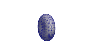
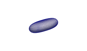
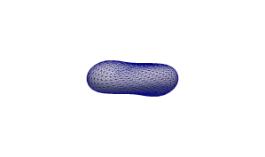
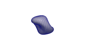
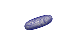
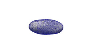
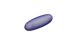
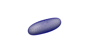
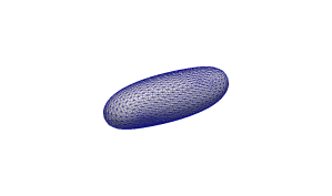
(b) Top to bottom: $\mu_{\Gamma}^{*}=3$, $1$, $0.1$ for $1/\alpha^{*}=10$ at times $t=0,\ 3,\ 6,\ 9$.

Figure 6: (Color online) Phase diagram for $\Lambda=1$ for the domain $\overline{\Omega}=[-3,3]^{3}$, starting with a biconcave shape with $\mathcal{V}_{r}=0.8$ and the shortest axis in the $x_{1}$-direction. The three big circles in the phase diagram correspond to the simulations in (b).

The evolutions for $\alpha^{*}=0.1$, and either $\mu_{\Gamma}^{*}=3$, $\mu_{\Gamma}^{*}=1$, or $\mu_{\Gamma}^{*}=0.1$, are visualized in Figure 6(b), where we observe the motions TU, TR and TT, respectively. We stress that the tumbling occurs for a viscosity contrast of $\Lambda=1$, and so is only due to the chosen high surface viscosity $\mu_{\Gamma}^{*}$. The fact that vesicles undergo a transition from steady tank treading to unsteady tumbling motion has been observed earlier by Noguchi and Gompper (2005b), where, however, the authors used a particle-based mesoscopic model to analyze the fluid vesicle dynamics. A plot of the inclination angle $\theta$ for the simulations in Figure 6(b) can be seen in Figure 7.

Figure 7: The inclination angle $\theta$ for the computations in Figure 6(b). They correspond to the motions TU, TR and TT, respectively.

IV.4 Effect of spontaneous curvature

Here the initial shapes of the vesicles, for a reduced volume of $\mathcal{V}_{r}=0.8$ and surface area $\mathcal{A}(0)=4\,\pi$, so that $S=1$, were chosen to be numerical approximations of local minimizers for the curvature energy $\int_{\Gamma}(\varkappa-\overline{\varkappa}^{*})^{2}\;{\rm d}s$. These discrete local minimizers were obtained with the help of the gradient flow scheme from Barrett et al. (2008), and for the choices $\overline{\varkappa}^{*}=\pm 5$ they are displayed in Figure 8.

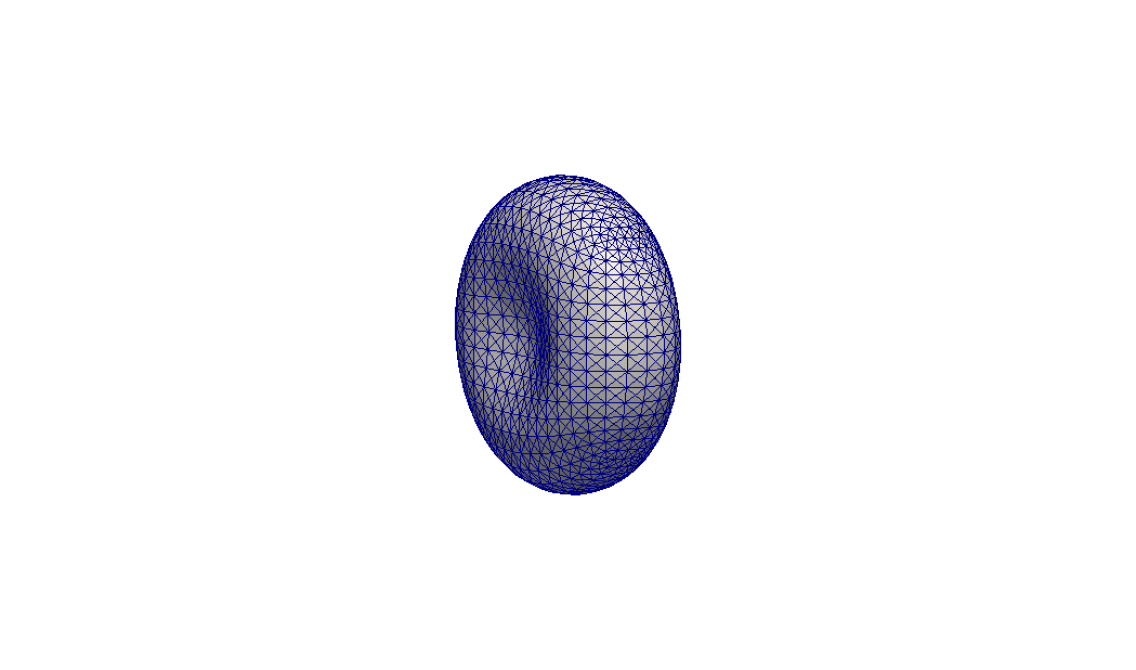
(a) $\overline{\varkappa}=-5$

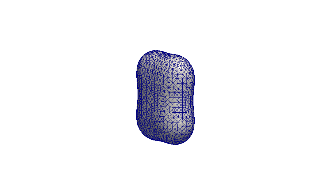
(b) $\overline{\varkappa}=5$

Figure 8: (Color online) The vesicles for $\overline{\varkappa}^{*}=\pm 5$ at time $t=0$.

For ${\rm Ca}=1/\alpha^{*}=10$ we show a phase diagram of $\mathcal{M}=\mu_{\Gamma}^{*}$ versus $\overline{\varkappa}^{*}$ in Figure 9, where the initial vesicles are aligned such that their shortest axis is in the $x_{1}$-direction.

Figure 9: (Color online) Phase diagram for ${\rm Ca}=1/\alpha^{*}=10$ for the domain $\overline{\Omega}=[-3,3]^{3}$, starting with biconcave shapes with $\mathcal{V}_{r}=0.8$ and the shortest axis in the $x_{1}$-direction.

Similarly, in Figure 10 we show a phase diagram of $\mathcal{M}=\mu_{\Gamma}^{*}$ versus $\overline{\varkappa}^{*}$ when the initial vesicles are aligned such that their shortest axis is in the $x_{2}$-direction.

Figure 10: Phase diagram for ${\rm Ca}=1/\alpha^{*}=10$ for the domain $\overline{\Omega}=[-3,3]^{3}$, starting with biconcave shapes with $\mathcal{V}_{r}=0.8$ and the shortest axis in the $x_{2}$-direction.

$\mu_{\Gamma}^{*}$	$\overline{\varkappa}^{*}=-5$	$\overline{\varkappa}^{*}=0$	$\overline{\varkappa}^{*}=5$
0.05	0.179	0.178	0.194
0.1	0.169	0.158	0.179
0.2	0.161	0.116	0.138

Table 1: Some inclination angles $\theta$ for the TT motions in Figure 9.

$\mu_{\Gamma}^{*}$	$\overline{\varkappa}^{*}=-5$	$\overline{\varkappa}^{*}=0$	$\overline{\varkappa}^{*}=5$
0.05	0.180	0.156	0.162
0.1	0.160	0.132	0.156
0.2	0.118	0.084	0.143

Table 2: Some inclination angles $\theta$ for the TT motions in Figure 10.

The results in Figures 9 and 10 indicate that the values of the surface viscosity, at which the transitions between TT, TR and TU take place, strongly depend on the spontaneous curvature as well as on the orientation of the initial vesicle. As in Noguchi and Gompper (2005b), where the case $\overline{\varkappa}^{*}=0$ was studied, we also observe that the inclination angle in the tank treading motion decreases as $\mu_{\Gamma}^{*}$ increases, see Tables 1 and 2.

IV.5 Shearing for a torus

Here we use as the initial shape a Clifford torus, that is aligned with the $x_{2}$-$x_{3}$ plane, with reduced volume $\mathcal{V}_{r}=0.71$ and $\mathcal{A}(0)=13.88$, so that $S=1.05$. We let $\Lambda=\mu_{\Gamma}^{*}=1$, $\alpha^{*}=0.05$ and use the domain $\overline{\Omega}=[-2,2]^{3}$. See Figure 11, where the torus appears to tumble whilst undergoing strong deformations.

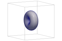
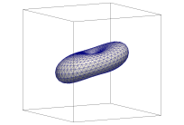
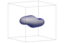
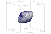
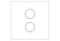
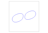
Figure 11: (Color online) Shear flow for a torus with $\Lambda=\mu_{\Gamma}^{*}=1$. The plots show the interface $\Gamma^{h}$ within $\overline{\Omega}$, as well as cuts through the $x_{1}$-$x_{3}$ plane, at times $t=0,\ 2.5,\ 5,\ 7.5$. The interface at $t=10$ is very close to the plot at $t=2.5$.

Repeating the experiment for an initial torus aligned with the shear flow direction, and setting $\alpha^{*}=1$ and $\mu_{\Gamma}^{*}=10$, leads to the results shown in Figure 12. This shows a TR motion.

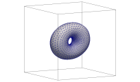
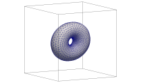
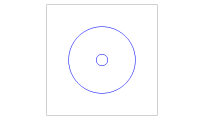
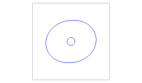
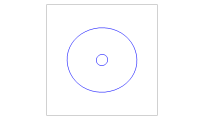
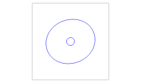
Figure 12: (Color online) Shear flow for a torus with $\Lambda=1$, $\mu_{\Gamma}^{*}=10$. The plots show the interface $\Gamma^{h}$ within $\overline{\Omega}$, as well as cuts through the $x_{1}$-$x_{3}$ plane, at times $t=0,\ 2.5,\ 5,\ 7.5$.

Setting $\mu_{\Gamma}^{*}=0$, on the other hand, leads to TT, as shown in Figure 13.

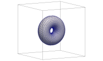
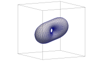
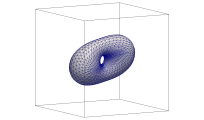
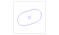
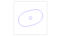
Figure 13: (Color online) Shear flow for a torus with $\Lambda=1$, $\mu_{\Gamma}^{*}=0$. The plots show the interface $\Gamma^{h}$ within $\overline{\Omega}$, as well as cuts through the $x_{1}$-$x_{3}$ plane, at times $t=0,\ 2.5,\ 5,\ 7.5$.

A plot of the inclination angle $\theta$ for the simulations in Figures 12 and 13 can be seen in Figure 14, while we visualize the flow in the $x_{1}$-$x_{3}$ plane in Figure 15.

Figure 14: The inclination angle $\theta$ for the simulations in Figures 12 and 13.

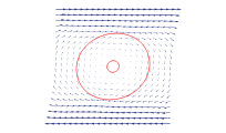
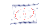
Figure 15: (Color online) The flow at time $t=7.5$ in the $x_{1}$-$x_{3}$ plane for the simulations in Figures 12 and 13.

IV.6 Effect of area difference elasticity

We consider $\overline{\Omega}=[-4,4]^{3}$ and set $\Lambda=\mu_{\Gamma}^{*}=\alpha^{*}=1$. The parameters for $\vec{f}_{\Gamma}^{*}$ are $\beta^{*}=0.053$ and $M_{0}^{*}=-48.24$. For the vesicle we use a cup-like stomatocyte initial shape with $\mathcal{V}_{r}=0.65$ and $\mathcal{A}(0)=82.31$, so that $S=2.56$. See Figure 16 for a numerical simulation. As a comparison, we show the same simulation with $\beta^{*}=0$ in Figure 17.

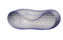
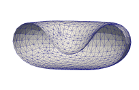
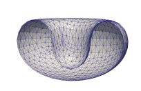
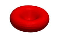
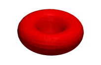
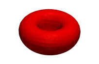
Figure 16: (Color online) Flow for a cup-like stomatocyte shape with $\mathcal{V}_{r}=0.65$ for $M_{0}^{*}=-48.24$ and $\beta^{*}=0.053$. The plots show the interface $\Gamma^{h}$ at times $t=0,\ 5,\ 10,\ 20$, with the top row visualizing the triangulations by showing half the vesicle.

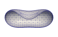
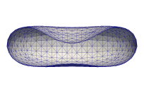
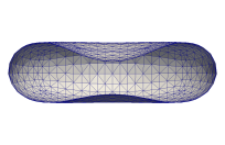
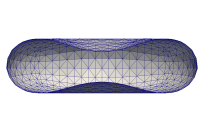
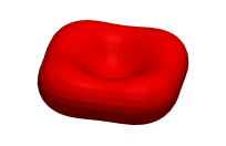
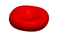
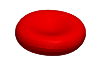
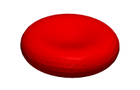
Figure 17: (Color online) Same as Figure 16 with $\beta^{*}=0$.

In Figure 18 we show the evolutions of the discrete volume of the inner phase and the discrete surface area over time. Clearly these two quantities are preserved almost exactly for our numerical scheme in this simulation. In fact, a semidiscrete variant of our scheme conserves these two quantities exactly, and so in practice the fully discrete algorithm will preserve them well for sufficiently small time step sizes.

Figure 18: The evolutions of the relative discrete volume $\mathcal{V}(t)/\mathcal{V}(0)$, and the relative discrete surface area $\mathcal{A}(t)/\mathcal{A}(0)$ over time.

In our next simulation, we let $\overline{\Omega}=[-2.5,2.5]^{3}$ and set $\Lambda=\alpha^{*}=1$, as well as $\beta^{*}=0.46$ and $M_{0}^{*}=-33.5$. As initial vesicle we take a varying-diameter cigar-like shape that has $\mathcal{V}_{r}=0.75$ and $\mathcal{A}(0)=9.65$, so that $S=0.88$. A simulation can be seen in Figure 19. As a comparison, we show the simulation with $\beta^{*}=0$ in Figure 20. Similarly to previous studies, where an energy involving area difference elasticity terms was minimized, we also observe in our hydrodynamic model that less symmetric shapes occur when the ADE-energy contributions are taken into account.

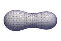
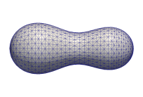
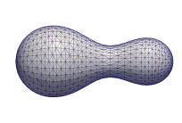
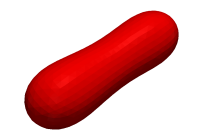
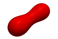
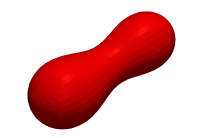
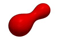
Figure 19: (Color online) Flow for a varying-diameter cigar-like shape with $\mathcal{V}_{r}=0.75$ for $M_{0}^{*}=-33.5$ and $\beta^{*}=0.46$. The plots show the interface $\Gamma^{h}$ at times $t=0,\ 1,\ 10,\ 50$, with the top row visualizing the triangulations.

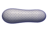
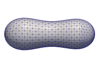
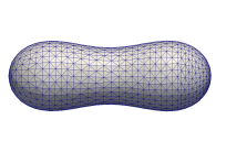
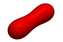
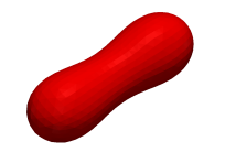
Figure 20: (Color online) Same as Figure 19 with $\beta^{*}=0$.

IV.7 Shearing for budded shape (two arms)

We start a scaled variant of the final shape from Figure 19 in a shear flow experiment in $\overline{\Omega}=[-2,2]^{3}$. In particular, the initial shape is axisymmetric, with reduced volume $\mathcal{V}_{r}=0.75$ and $\mathcal{A}(0)=5.43$, so that $S=0.66$. We set $\Lambda=\mu_{\Gamma}^{*}=1$, $\alpha^{*}=0.05$. See Figure 21 for a run with $\beta^{*}=0.1$ and $M_{0}^{*}=-33.5$. We observe that the shape of the vesicle changes drastically, with part of the surface growing inwards. This is similar to the shapes observed in Figure 16, where the presence of a lower reduced volume led to cup-like stomatocyte shapes.

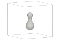
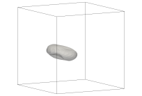
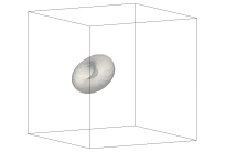
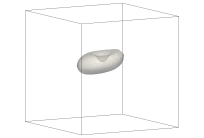
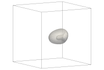
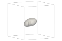
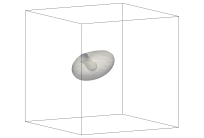
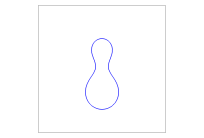
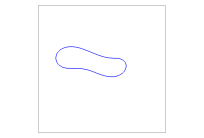
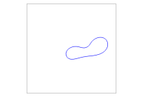
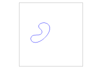
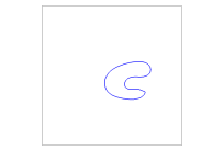
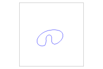
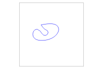
Figure 21: (Color online) Shear flow for a budding shape with $\Lambda=\mu_{\Gamma}^{*}=1$. Here $\beta^{*}=0.1$ and $M_{0}^{*}=-33.5$. The plots show the interface $\Gamma^{h}$ within $\overline{\Omega}$, as well as cuts through the $x_{1}$-$x_{3}$ plane, at times $t=0,\ 5,\ 15,\ 17.5,\ 20,\ 25,\ 27.5,\ 32.5$.

We repeat the same experiment for $\beta^{*}=0$ in Figure 22. Now the budding shape loses its strong nonconvexity completely, as can be clearly seen in the plots of the two-dimensional cuts in Figure 22. Plots of the bending energy $\alpha^{*}\,E^{*}(\Gamma^{h})$ are shown in Figure 23, where we recall that the energy inequality in (3) does not hold for the inhomogeneous boundary conditions employed in the present simulations.

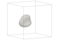
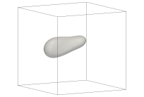
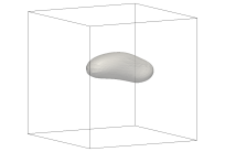
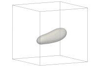
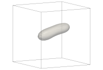
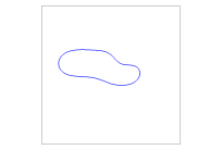
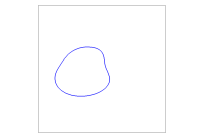
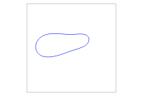
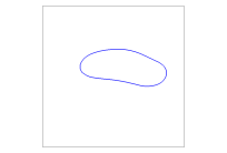
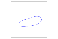
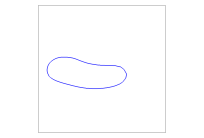
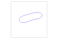
Figure 22: (Color online) Same as Figure 21 but with $\beta^{*}=0$.

Figure 23: The bending energy $\alpha^{*}\,E^{*}(\Gamma^{h})$ for the computations in Figures 21 and 22.

IV.8 Shearing for a seven-arm starfish

We consider simulations for a scaled version of the final shape from Barrett et al. (2008, Fig. 23) with reduced volume $\mathcal{V}_{r}=0.38$ and $\mathcal{A}(0)=10.54$, so that $S=0.92$, inside the domain $\overline{\Omega}=[-2,2]^{3}$. We set $\Lambda=\mu_{\Gamma}^{*}=\alpha^{*}=1$. In order to maintain the seven-arm shape during the evolution we set $\beta^{*}=0.05$ and $M_{0}^{*}=180$. The first experiment is for no-slip boundary conditions on $\partial\Omega$ and shows that the seven arms grow slightly, see Figure 24.

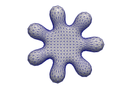
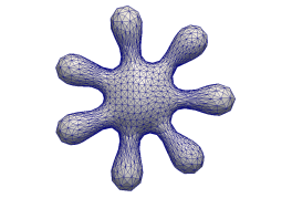
Figure 24: (Color online) Flow for a seven-arm figure with $\mathcal{V}_{r}=0.38$. Here $\beta^{*}=0.05$ and $M_{0}^{*}=180$. The triangulations $\Gamma^{h}$ at times $t=0$ and $5$.

If we use the shear flow boundary conditions, on the other hand, we observe the behaviour in Figure 25, where we have changed the value of $\alpha^{*}$ to $0.05$. The vesicle can be seen tumbling, with a tumbling period of about $7$, with the seven arms remaining intact throughout.

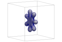
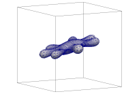
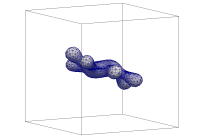
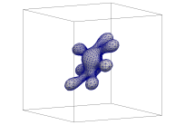
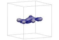
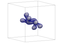
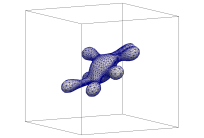
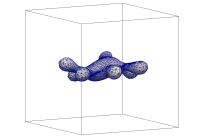
Figure 25: (Color online) Shear flow for a budding shape with $\Lambda=\mu_{\Gamma}^{*}=1$. Here $\beta^{*}=0.05$ and $M_{0}^{*}=180$. The plots show the interface $\Gamma^{h}$ within $\overline{\Omega}$ at times $t=0,\ 2.5,\ 5,\ 7.5,\ 10,\ 12.5,\ 15,\ 17.5$.

Repeating the same experiment with $\beta^{*}=0$ yields the simulation in Figure 26. Not surprisingly, some of the arms of the vesicle are disappearing.

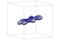
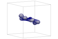
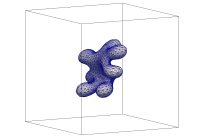
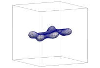
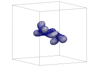
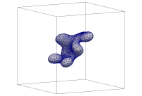
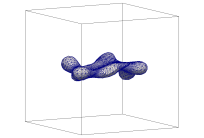
Figure 26: (Color online) Same as Figure 25 with $\beta^{*}=0$.

We also tried to investigate whether the arms enhance or inhibit the tumbling behaviour of the vesicle. To this end, we repeated the simulation in Figure 25 for an ellipsoidal vesicle with the same reduced volume and surface area. This vesicle also exhibited TU with a tumbling period of about $7$, so there was no significant change to the behaviour in Figure 25.

V Conclusions

We have introduced a parametric finite element method for the evolution of bilayer membranes by coupling a general curvature elasticity model for the membrane to (Navier–)Stokes systems in the two bulk phases and to a surface (Navier–)Stokes system. The model is based on work by Arroyo and DeSimone (2009), which we generalized such that area difference elasticity effects (ADE) are taken into account. Our main purpose was to study the influence of the area difference elasticity and of the spontaneous curvature on the evolution of the membrane. In contrast to most other works, we discretized the full bulk (Navier–)Stokes systems coupled to the surface (Navier–)Stokes system and for the first time coupled this to a bending energy involving ADE and spontaneous curvature.

The numerical simulations led to the following findings.

• The proposed numerical method conserves the volume enclosed by the membrane and the surface area of the membrane to a high precision.

• The transition from a tank treading (TT) motion to a transition motion (TR) and to a tumbling (TU) motion depended strongly on the surface viscosity. We observed that the surface viscosity alone with no viscosity contrast between inner and outer fluid can lead to a transition from tank treading to a TR-motion and to tumbling. Similar observations have been reported by Noguchi and Gompper (2005b) using a particle-based method.

• The surface viscosity at which a transition between the different motions TT, TR and TU occur, strongly depends on the spontaneous curvature and on the initial alignment of the vesicle. In particular, we observed that for negative spontaneous curvature and an initial biconcave vesicle aligned such that the shortest axis is in the shear flow direction all transitions occurred for larger values of the surface viscosity. For this alignment, and for positive spontaneous curvature, we observed that tumbling occurred already for much smaller values of the surface viscosity. The reverse was true for an alternative alignment. Here we recall that our sign convention for curvature means that spheres have negative mean curvature.

• In some cases, shear flow can lead to drastic shape changes, in particular for the ADE-model. For example, we observed the transition of a budded pear-like shape to a cup-like stomatocyte shape in shear flow if an ADE-model was used for the curvature elasticity.

• The ADE-model can also lead to starfish-type shapes with several arms, see e.g. Wintz et al. (1996); Seifert (1997). In computations for a seven-arm starfish for a model involving an ADE type energy, we observed that in shear flow the overall structure seems to be quite robust. In particular, the seven arms deformed but remained present even in a tumbling motion. However, arms tend to disappear if the area difference elasticity term is neglected.

Thus we have shown that the proposed numerical method is a robust tool to simulate bilayer membranes for quite general models which in particular take the full hydrodynamics and a curvature model involving area difference elasticity and spontaneous curvature into account.

Acknowledgement. The authors gratefully acknowledge the support of the Deutsche Forschungsgemeinschaft via the SPP 1506 entitled “Transport processes at fluidic interfaces” and of the Regensburger Universitätsstiftung Hans Vielberth.

References

- Seifert (1997) U. Seifert, Adv. Phys. 46, 13 (1997).
- Baumgart et al. (2003) T. Baumgart, S. T. Hess, and W. W. Webb, Nature 425, 821 (2003).
- Noguchi and Gompper (2005a) H. Noguchi and G. Gompper, PNAS 102, 14159 (2005a).
- McWhirter et al. (2009) J. L. McWhirter, H. Noguchi, and G. Gompper, Proc. Natl. Acad. Sci. USA 106, 6039 (2009).
- Canham (1970) P. Canham, J. Theor. Biol. 26, 61 (1970).
- Helfrich (1973) W. Helfrich, Z. Naturforsch. 28c, 693 (1973).
- Martens and McMahon (2008) S. Martens and H. T. McMahon, Nat. Rev. Mol. Cell. Biol. 9, 543 (2008).
- Kamal et al. (2009) M. M. Kamal, D. Mills, M. Grzybek, and J. Howard, PNAS 106, 22245 (2009).
- Svetina et al. (1982) S. Svetina, A. Ottova-Leitmannová, and R. Glaser, J. Theor. Biol. 94, 13 (1982).
- Svetina and Zeks (1983) S. Svetina and B. Zeks, Biomed. Biochim. Acta 42, 86 (1983).
- Svetina and Zeks (1989) S. Svetina and B. Zeks, Eur. Biophys. J. 17, 101 (1989).
- Miao et al. (1994) L. Miao, U. Seifert, M. Wortis, and H.-G. Döbereiner, Phys. Rev. E 49, 5389 (1994).
- Ziherl and Svetina (2005) P. Ziherl and S. Svetina, Europhys. Lett. 70, 690 (2005).
- Seifert et al. (1991) U. Seifert, K. Berndl, and R. Lipowsky, Phys. Rev. A 44, 1182 (1991).
- Wintz et al. (1996) W. Wintz, H.-G. Döbereiner, and U. Seifert, Europhys. Lett. 33, 403 (1996).
- Mayer and Simonett (2002) U. F. Mayer and G. Simonett, Interfaces Free Bound. 4, 89 (2002).
- Clarenz et al. (2004) U. Clarenz, U. Diewald, G. Dziuk, M. Rumpf, and R. Rusu, Comput. Aided Geom. Design 21, 427 (2004).
- Dziuk (2008) G. Dziuk, Numer. Math. 111, 55 (2008).
- Barrett et al. (2008) J. W. Barrett, H. Garcke, and R. Nürnberg, SIAM J. Sci. Comput. 31, 225 (2008).
- Du et al. (2005) Q. Du, C. Liu, R. Ryham, and X. Wang, Nonlinearity 18, 1249 (2005).
- Franken et al. (2013) M. Franken, M. Rumpf, and B. Wirth, Int. J. Numer. Anal. Model. 10, 116 (2013).
- Bonito et al. (2010) A. Bonito, R. H. Nochetto, and M. S. Pauletti, J. Comput. Phys. 229, 3171 (2010).
- Du et al. (2004) Q. Du, C. Liu, and X. Wang, J. Comput. Phys. 198, 450 (2004).
- Elliott and Stinner (2010) C. M. Elliott and B. Stinner, J. Comput. Phys. 229, 6585 (2010).
- Bartels et al. (2012) S. Bartels, G. Dolzmann, R. H. Nochetto, and A. Raisch, Interfaces Free Bound. 14, 231 (2012).
- Mercker et al. (2013) M. Mercker, A. Marciniak-Czochra, T. Richter, and D. Hartmann, SIAM J. Appl. Math. 73, 1768 (2013).
- Du et al. (2009) Q. Du, C. Liu, R. Ryham, and X. Wang, Phys. D 238, 923 (2009).
- Boedec et al. (2011) G. Boedec, M. Leonetti, and M. Jaeger, J. Comput. Phys. 230, 1020 (2011).
- Rahimi and Arroyo (2012) M. Rahimi and M. Arroyo, Phys. Rev. E 86, 011932 (2012).
- Rodrigues et al. (2015) D. S. Rodrigues, R. F. Ausas, F. Mut, and G. C. Buscaglia, J. Comput. Phys. 298, 565 (2015).
- Salac and Miksis (2011) D. Salac and M. Miksis, J. Comput. Phys. 230, 8192 (2011).
- Salac and Miksis (2012) D. Salac and M. J. Miksis, J. Fluid Mech. 711, 122 (2012).
- Laadhari et al. (2014) A. Laadhari, P. Saramito, and C. Misbah, J. Comput. Phys. 263, 328 (2014).
- Doyeux et al. (2013) V. Doyeux, Y. Guyot, V. Chabannes, C. Prud’homme, and M. Ismail, J. Comput. Appl. Math. 246, 251 (2013).
- Biben et al. (2005) T. Biben, K. Kassner, and C. Misbah, Phys. Rev. E 72, 041921 (2005).
- Jamet and Misbah (2007) D. Jamet and C. Misbah, Phys. Rev. E 76, 051907 (2007).
- Aland et al. (2014) S. Aland, S. Egerer, J. Lowengrub, and A. Voigt, J. Comput. Phys. 277, 32 (2014).
- Kim and Lai (2010) Y. Kim and M.-C. Lai, J. Comput. Phys. 229, 4840 (2010).
- Kim and Lai (2012) Y. Kim and M.-C. Lai, Phys. Rev. E 86, 066321 (2012).
- Hu et al. (2014) W.-F. Hu, Y. Kim, and M.-C. Lai, J. Comput. Phys. 257, 670 (2014).
- Dodson and Dimitrakopoulos (2011) W. R. Dodson and P. Dimitrakopoulos, Phys. Rev. E 84, 011913 (2011).
- Farutin et al. (2014) A. Farutin, T. Biben, and C. Misbah, J. Comput. Phys. 275, 539 (2014).
- Arroyo and DeSimone (2009) M. Arroyo and A. DeSimone, Phys. Rev. E 79, 031915 (2009).
- Arroyo et al. (2010) M. Arroyo, A. DeSimone, and L. Heltai, (2010), arXiv:1007.4934 .
- Barrett et al. (2014) J. W. Barrett, H. Garcke, and R. Nürnberg, “A stable numerical method for the dynamics of fluidic biomembranes,” (2014), preprint No. 18/2014, University Regensburg, Germany.
- Barrett et al. (2015a) J. W. Barrett, H. Garcke, and R. Nürnberg, “Finite element approximation for the dynamics of asymmetric fluidic biomembranes,” (2015a), preprint No. 03/2015, University Regensburg, Germany.
- Seifert et al. (1992) U. Seifert, L. Miao, H.-G. Döbereiner, and M. Wortis, in The Structure and Conformation of Amphiphilic Membranes, Springer Proceedings in Physics, Vol. 66, edited by R. Lipowsky, D. Richter, and K. Kremer (Springer-Verlag, Berlin, 1992) pp. 93–96.
- Wiese et al. (1992) W. Wiese, W. Harbich, and W. Helfrich, J. Phys. Condens. Matter 4, 1647 (1992).
- Bozic et al. (1992) B. Bozic, S. Svetina, B. Zeks, and R. Waugh, Biophys. J. 61, 963 (1992).
- Scriven (1960) L. E. Scriven, Chem. Eng. Sci. 12, 98 (1960).
- Willmore (1965) T. J. Willmore, An. Şti. Univ. “Al. I. Cuza” Iaşi Secţ. I a Mat. (N. S.) 11B, 493 (1965).
- Faivre (2006) M. Faivre, Drops, vesicles and red blood cells: Deformability and behavior under flow, Ph.D. thesis, Université Joseph Fourier, Grenoble, France (2006).
- Abreu et al. (2014) D. Abreu, M. Levant, V. Steinberg, and U. Seifert, Adv. Colloid Interface Sci. 208, 129 (2014).
- Spann et al. (2014) A. P. Spann, H. Zhao, and E. S. G. Shaqfeh, Phys. Fluids 26, 031902 (2014).
- Bänsch (2001) E. Bänsch, Numer. Math. 88, 203 (2001).
- Capovilla and Guven (2004) R. Capovilla and J. Guven, J. Phys. Condens. Matter 16, 2187 (2004).
- Lengeler (2015) D. Lengeler, (2015), arXiv:1506.08991 .
- Barrett et al. (2015b) J. W. Barrett, H. Garcke, and R. Nürnberg, J. Sci. Comp. 63, 78 (2015b).
- Ramanujan and Pozrikidis (1998) S. Ramanujan and C. Pozrikidis, J. Fluid Mech. 361, 117 (1998).
- Misbah (2006) C. Misbah, Phys. Rev. Lett. 96, 028104 (2006).
- Kantsler and Steinberg (2006) V. Kantsler and V. Steinberg, Phys. Rev. Lett. 96, 036001 (2006).
- Zabusky et al. (2011) N. J. Zabusky, E. Segre, J. Deschamps, V. Kantsler, and V. Steinberg, Phys. Fluids 23, 041905 (2011).
- Noguchi and Gompper (2007) H. Noguchi and G. Gompper, Phys. Rev. Lett. 98, 128103 (2007).
- Yazdani and Bagchi (2012) A. Yazdani and P. Bagchi, Phys. Rev. E 85, 056308 (2012).
- Farutin and Misbah (2012) A. Farutin and C. Misbah, Phys. Rev. Lett. 109, 248106 (2012).
- Biben et al. (2011) T. Biben, A. Farutin, and C. Misbah, Phys. Rev. E 83, 031921 (2011).
- Kaoui et al. (2012) B. Kaoui, T. Krüger, and J. Harting, Soft Matter 8, 9246 (2012).
- Noguchi and Gompper (2005b) H. Noguchi and G. Gompper, Phys. Rev. E 72, 011901 (2005b).