Nonparametric Testing for Heterogeneous Correlation

Abstract.

In the presence of weak overall correlation, it may be useful to investigate if the correlation is significantly and substantially more pronounced over a subpopulation. Two different testing procedures are compared. Both are based on the rankings of the values of two variables from a data set with a large number n of observations. The first maintains its level against Gaussian copulas; the second adapts to general alternatives in the sense that that the number of parameters used in the test grows with $n$. An analysis of wine quality illustrates how the methods detect heterogeneity of association between chemical properties of the wine, which are attributable to a mix of different cultivars.

Introduction

The goal of this paper is to offer new methods for discovering association between two variables that is supported only in a subpopulation. For example, while higher counts of HDLs are generally associated with lower risk of myocardial infarction, researchers (Voight et al., 2012; Katz, 2014) have found subpopulations that do not adhere to this trend. In marketing, subpopulations of designated marketing areas (DMAs) in the US respond differentially to TV advertising campaigns, and the identification of DMAs that are sensitive to ad exposure enables efficient spending of ad dollars. In preclinical screening of potential drugs, various subpopulations of chemicals elicit concomitant responses from sets of hepatocyte genes, which can be used to discover gene networks that breakdown classes of drugs, without having to pre-specify how the classes are formed. The new methods thus lead to a whole new approach to analysis of large data sets.

When covariates are available, regression analysis classically attempts to identify a supporting subpopulation via interaction effects, but these may be difficult to interpret properly. In the presence of overall correlation, it may be useful to investigate directly if the correlation is significantly and substantially more pronounced over a subpopulation. This becomes feasible when representatives of supporting subpopulations are embedded in large samples. The novel statistical tests described in this paper are designed to probe large samples to ascertain if there is such a subpopulation.

The general setting is this: A large number n of observations are sampled from a bivariate continuous distribution. The basic assumption is that the population consists of two subpopulations. In one, the two variables are positively (or negatively) associated; in the other, the two variables are independent. While some distributional assumptions are required even to define the notion of homogeneous association, the underlying intent is to make the tests robust to assumptions about the distributions governing both the null and alternative hypotheses.

Notation for the rest of the paper is as follows: Let $X\sim F$ and $Y\sim G$ have joint, continuous distribution H. For any sample $\left\{\left(x_{i},y_{i}\right)\mid i=1,\ldots,n\right\}$, the empirical marginal distributions are defined by

$$\hat{F}_{n}\left(x\right)=\frac{1}{n}\sum_{i=1}^{n}1\left\{x_{i}\leq x\right\} \hat{G}_{n}\left(y\right)=\frac{1}{n}\sum_{i=1}^{n}1\left\{y_{i}\leq y\right\}.$$ and

The ranking $\pi$ of the sample $\left\{x_{i}\mid i=1,\ldots,n\right\}$ is the function
$\pi:\left\{x_{i}\mid i=1,\ldots,n\right\}\rightarrow\left\{1,\ldots,n\right\}$ defined by

$$\pi\left(x_{i}\right)=\sum_{j=1}^{n}1\left\{x_{i}\leq x_{j}\right\}.$$

The corresponding ranking of $\left\{y_{i}\mid i=1,\ldots,n\right\}$ is denoted by $\nu$. Spearman’s footrule distance with a sample $\left\{\left(x_{i},y_{i}\right)\mid i=1,\ldots,n\right\}$ is defined through the sample rankings as

$$d_{S}=\sum_{i=1}^{n}\left|\pi\left(x_{i}\right)-\nu\left(y_{i}\right)\right|.$$

The Kendall distance associated with the sample is defined as

$$D_{K}\left(\left[x_{1},\ldots,x_{n}\right],\left[y_{1},\ldots,y_{n}\right]\right) = \sum_{i<j}1\left\{\left(x_{i}-x_{j}\right)\left(y_{i}-y_{j}\right)<0\right\}$$

$$= \sum_{i<j}1\left\{\left(\pi\left(x_{i}\right)-\pi\left(x_{j}\right)\right)\left(\nu\left(y_{i}\right)-\nu\left(y_{j}\right)\right)<0\right\}$$

$$= d_{K}\left(\pi,\nu\right)$$

which depends only on the rankings $\pi$ and $\nu$ of the sample $\left\{x_{i}\right\}$ and $\left\{y_{i}\right\}$. Mallows (1957) model for rankings takes the form

$$P_{\phi}\left(\nu\mid\pi\right)=C\left(\phi\right)e^{-\phi d_{K}\left(\pi,\nu\right)}$$

where the normalizing constant $C\left(\phi\right)$ has a tractable form (Fligner and Verducci, 1986) known as a Poincare polynomial (Diaconis and Graham, 2000). Distributional forms for the data are in terms of copulas:

$$C_{H}\left(F\left(X\right),G\left(Y\right)\right)=H\left(X,Y\right)$$

which are distribution functions on the unit square, having uniform margins. Two copulas play a fundamental role in motivating the tests: the Gaussian copula and the Frank Copula. If $\left(X,Y\right)$ has a bivariate normal distribution $H$ with correlation $\rho$, then its corresponding copula is

$$C_{\rho}\left(u,v\right)=\Phi_{2}\left(\Phi^{-1}\left(u\right),\Phi^{-1}\left(v\right);\rho\right)$$

where $\Phi$ is the standard normal CDF. The bivariate distributions $C_{\rho}$ and $\Phi_{2}$ are indexed solely by the underlying correlation $\rho$. The Frank copula (Frank, 1979; Genest, 1987) has the form

$$C_{\theta}\left(u,v\right)=-\frac{1}{\theta}\log\left(1+\frac{\left(e^{-\theta u}-1\right)\left(e^{-\theta v}-1\right)}{\left(e^{-\theta}-1\right)}\right).$$

The next two sections describe two new tests for detecting subpopulations that support association: the Components of Spearman’s Footrule (CSF) test and the Components of Kendall’s Tau (CKT) test. The CSF test is scaled according to a Gaussian copula and the CKT test is scaled according to a Frank copula. The CSF test is computationally fast, and the CKT test adapts to a large variety of alternatives. The following two sections cover their performance under simulations. Concluding remarks are in last section.

Components of Spearman’s Footrule (CSF)

While Spearman’s footrule (Diaconis and Graham, 1977) measures the overall disarray in a sample, the distribution of individual absolute rank differences

$$d_{i}=\left|\pi\left(x_{i}\right)-\nu\left(y_{i}\right)\right|$$

proves to be very useful in detecting subsamples with distinctly less disarray than would be expected under homogeneous association. Because the rankings depend on the whole sample, the $\left\{d_{i}\right\}$ are not independent. Nevertheless, we loosely define their empirical distribution as

$$S_{n}\left(d\right)=\frac{1}{n}\sum_{i=1}^{n}1\left\{d_{i}\leq d\right\}.$$

As a step toward determining asymptotic forms for this distribution, we offer the following lemmas.

Lemma 1.

For any sample $\left\{\left(X_{i},Y_{i}\right)\mid i=1,\ldots,n\right\}$, from a joint distribution $H$ with compact support, let (X,Y) be a newly, independent sampled observation. Then, for rankings $\pi$ and $\nu$ for the extended sample of $n+1$ observations,

$$\left[\frac{\pi\left(X\right)}{n+1},\frac{\nu\left(Y\right)}{n+1}\right]\underset{a.s.}{\rightarrow}\left[F\left(X\right),G\left(Y\right)\right]$$

and its asymptotic distribution is the underlying copula $C_{H}\left[F\left(X\right),G\left(Y\right)\right]$ of $H$.

Lemma 2.

Under independence, the asymptotic distribution of the scaled absolute rank differences

$$S_{n}=\left|\frac{\pi\left(X\right)}{n+1}-\frac{\nu\left(Y\right)}{n+1}\right|$$

is Beta$\left(1,2\right)$.

Proposition 3.

Under a Gaussian($\rho$) copula, $S_{n}$ converges to a Beta$\left(1,\beta\left(\rho\right)\right)$ distribution.

Although we do not have a formal proof for this proposition, many simulations with $n=1000$ affirm the proposition and produce a smooth curve for $\beta\left(\rho\right)$. See Figure 1 for one such example.

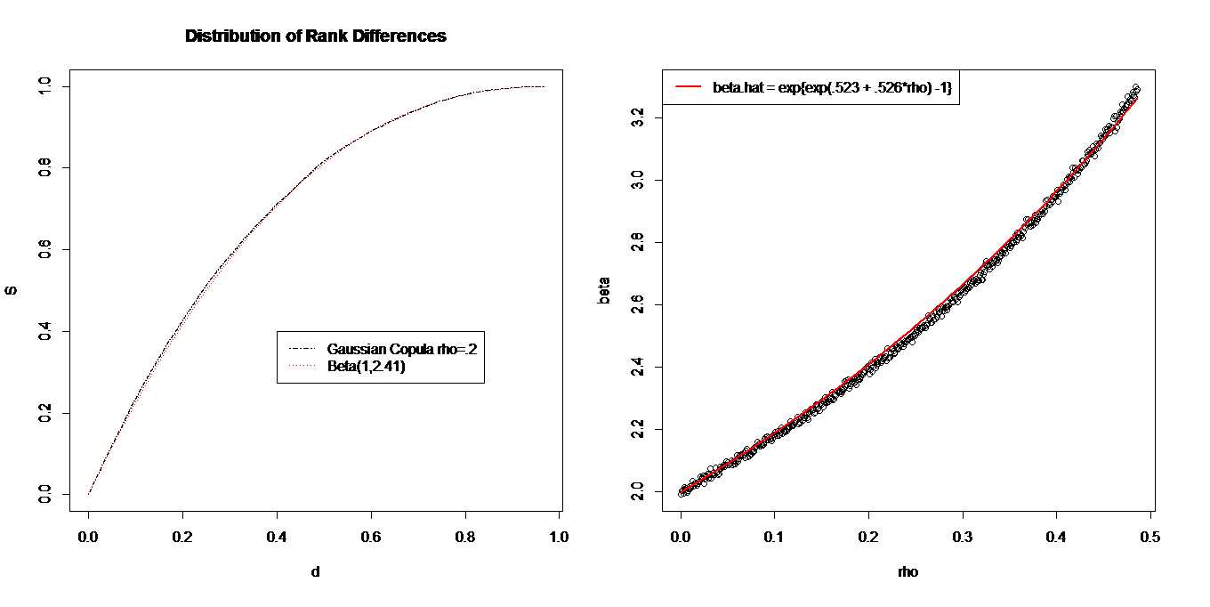
Figure 1. Left panel shows the close agreement of $S_{n}$ with Beta$\left(1,\beta\left(\rho\right)\right)$ when sampling $n=10,000$ observations from a Gaussian($\rho=0.2$) copula. The right panel illustrates the $\mathbf{\beta\left(\rho\right)}$ curve for $0<\rho<0.5$.

The null hypothesis is that $\left(X,Y\right)$ have a Gaussian copula. The alternative is that $\left(X,Y\right)$ come from a mixture of two subpopulations in which under one they are independent, and under the other they are positively associated. To test for negative association, simply replace $Y$ by $-Y$. No particular form is assumed for the positively associated subpopulation, but it is informative to examine the case where this component is Gaussian. Figure 2 illustrates $S_{n}$ and its histogram under such a mixture.

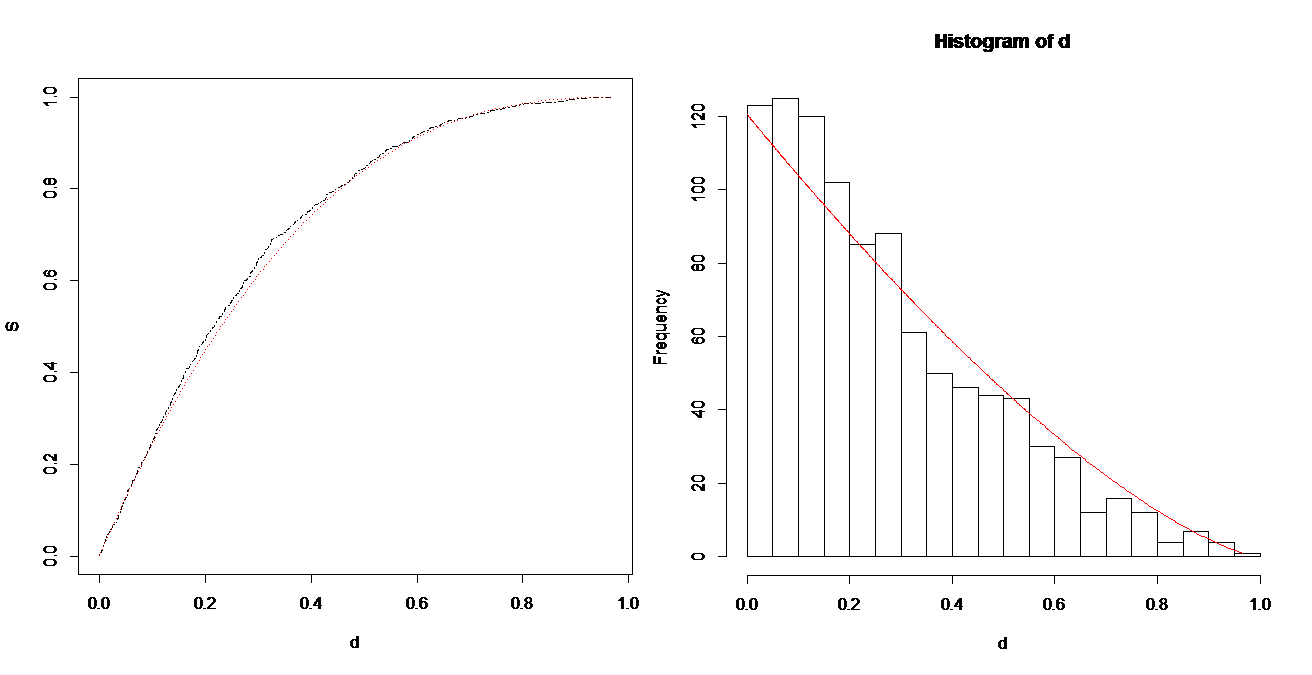
Figure 2. (Standardized) Distribution of Rank Differences Under Mixture of Gaussian(0.6) and Independent Copulas with overall correlation 0.3 compared to Beta(1,2.65).

Because the differences in distributions under the null and alternative are small, large samples are required to distinguish the two. As noted from the histogram in Figure 2, most of the distinguishing information is contained at the low end of the distribution. This makes sense because a subpopulation supporting positive association should have a surplus of points where the ranks of $X$ and $Y$ closely agree. Thus a test statistic based on absolute ranked differences should emphasize the lower order statistics. Such statistics come under the heading of L-statistics. It is possible to tailor a test toward alternative features of interest such as proportionate size of the subpopulation and the strength of association within it. Exact distributions of partial or weighted sums of absolute rank differences are quite complicated due to dependencies (Sen, et al. 2011), even under the null hypothesis of independence. A very simple general purpose test statistic is

$$T_{S}=\sum_{i=1}^{n}1\left\{\frac{\left|\pi\left(x_{i}\right)-\nu\left(y_{i}\right)\right|}{n}<0.2\right\}.$$

Using the observed overall correlation r in place of $\rho$, the null distribution of $T_{S}$ may be simulated under the Gaussian copula or approximated as a Binomial test statistic using the probability from the $\textrm{Beta}(1,\beta)$ as in Proposition 3. In the later case, ignoring weak dependencies, the .05 level test has power of 80% of detecting a Gaussian subpopulation of 25% with r =.8 for n = 1000.

Components of Kendall’s Tau (CKT)

Although the CSF test is both simple and computationally efficient, it has a conceptual shortcoming arising from the use of Spearman’s footrule distance to characterize association in a subpopulation. The issue is that the components of the footrule distance in the subpopulation depend on the encompassing population; that is, when the sample is a full population, with associated subpopulation $\Omega$, the component set from the footrule from $\Omega$

$$\left\{d_{i}\mid i\in\Omega\right\}=\left\{\left|\pi\left(x_{i}\right)-\nu\left(y_{i}\right)\right|\mid i\in\Omega\right\}$$

depends heavily on the rankings $\pi$ and $\nu$ determined by the full population. In contrast, the component set from Kendall’s distance depends only on the relative rankings within $\Omega$, which may be constructed from just on the original values in $\Omega$. That is,

$$\left\{1\left[\left(\pi\left(x_{i}\right)-\pi\left(x_{j}\right)\right)\left(\nu\left(y_{i}\right)-\nu\left(y_{j}\right)\right)<0\right]\mid i,j\in\Omega\right\}$$

$$=\left\{1\left[\left(x_{i}-x_{j}\right)\left(y_{i}-y_{j}\right)<0\right]\mid i,j\in\Omega\right\}$$

Thus the subpopulation discordances (components of Kendall’s distance) do not depend upon the embedding population, whereas the subpopulation disarray (components of Spearman’s footrule distance) do. This invariance has a number of beneficial properties, such as allowing the CKT test to retain power in situations where the ranges of the $\left\{X_{i}\right\}$ and $\left\{Y_{i}\right\}$ values in the subpopulation are more restricted than those in the full population.

The notion of homogeneous association based on Kendall’s distance differs from that based the Spearman’s footrule used for the CSF test. In this case the natural null hypothesis should be a distribution depending only on Kendall’s distance. Furthermore it should have the greatest entropy for a given value of Kendall’s tau because this formulation would attribute as much variability as possible to the null distribution, making it a conservative (least favorable) test (Lehmann and Romano, 2006). To construct a distribution that has this structure, simply sample from an arbitrary copula, and then reorder the Y-values according to a permutation $\nu\left(\mathbf{Y}\right)$ sampled independently from a Mallows model centered at the ranking $\pi\left(\mathbf{X}\right)$ of the X-values. Quite remarkably, any such process asymptotically leads to a Frank copula. Proposition 4, based on Starr (2009), gives a precise statement.

Proposition 4.

Let $\left\{\left(X_{i},Y_{i}\right)\mid i=1,\ldots,n\right\}$ be independent samples from a distribution $H$ with continuous marginals $F$ and $G$, and associated copula $C$ with continuous partial derivatives. Let $\pi\left(\mathbf{X}\right)$ be the ranking of $\pi\left(\mathbf{X}\right)=\left[X_{1},\ldots,X_{n}\right]$ and $\nu\left(\mathbf{Y}\right)$ be the ranking of $\nu\left(\mathbf{Y}\right)=\left[Y_{1},\ldots,Y_{n}\right]$ . Assume that for all $n$ sufficiently large, the conditional distribution of $\nu\left(\mathbf{Y}\right)$ given $\pi\left(\mathbf{X}\right)$ is Mallows, with center at $\pi\left(\mathbf{X}\right)$ and scale $\phi_{n}$. If $\phi_{n}\rightarrow 0$, and there exists $\theta\neq 0$ such that

$$n\left(1-e^{-\phi_{n}}\right)\rightarrow\theta,$$

then $C$ is the Frank Copula $C_{\theta}$.

Proof.

First, we establish that if the conditional distribution of $\nu\left(\mathbf{Y}\right)$ given $\pi\left(\mathbf{X}\right)$ is a Mallows distribution, then the copula C is radially symmetric. The pseudo-observations for each pair $\left(X_{i},Y_{i}\right)$ are defined as functions of the pair and the empirical margins

$$\left(\hat{U}_{i},\hat{V}_{i}\right) = \frac{n}{n+1}\left(\hat{F}_{n}\left(X_{i}\right),\hat{G}_{n}\left(Y_{i}\right)\right).$$

These are functions of the rankings $\pi\left(\mathbf{X}\right)$ and $\nu\left(\mathbf{Y}\right)$ :

$$\hat{U}_{i}=1-\frac{\pi\left(X_{i}\right)}{n+1}, \hat{V}_{i}=1-\frac{\nu\left(Y_{i}\right)}{n+1}.$$

By the symmetry of the Mallows model, the joint distribution of the pseudo-observations $\left(\hat{U}_{1},\hat{V}_{1}\right),\ldots,\left(\hat{U}_{n},\hat{V}_{n}\right)$ is identical to the joint distribution of
$\left(1-\hat{U}_{1},1-\hat{V}_{1}\right),\ldots,\left(1-\hat{U}_{n},1-\hat{V}_{n}\right)$ . Consider empirical distributions based on these observations (Genest and Nešlehová, 2014):

$$\hat{C}_{n}\left(u,v\right) = \frac{1}{n}\sum_{i=1}^{n}1\left\{\hat{U}_{i}\leq u,\hat{V}_{i}\leq v\right\}$$

$$\hat{D}_{n}\left(u,v\right) = \frac{1}{n}\sum_{i=1}^{n}1\left\{1-\hat{U}_{i}\leq u,1-\hat{V}_{i}\leq v\right\}.$$

Since $H$ has continuous marginals and $C$ has continuous partial derivatives, then Fermanian et al. (2004) established that $\hat{C}_{n}$ is a consistent estimator of the copula $C$, and likewise $\hat{D}_{n}$ is a consistent estimator of the survival copula $\bar{C}$, where

$$\bar{C}\left(u,v\right) = u+v-1+C\left(1-u,1-v\right).$$

Hence, $\bar{C}=C$, which implies that the copula $C$ is radially symmetric (Nelsen 2006, pg. 37). Since $C$ is radially symmetric, an asymptotically equivalent definition of the empirical copula is

$$\tilde{C}_{n}\left(u,v\right) = \frac{1}{n}\sum_{i=1}^{n}1\left\{\frac{\pi\left(X_{i}\right)}{n}\leq u,\frac{\nu\left(Y_{i}\right)}{n}\leq v\right\}$$

$$= \frac{1}{n}\sum_{i=1}^{n}\delta_{\left(\pi\left(X_{i}\right)/n,\nu\left(Y_{i}\right)/n\right)}$$

which places mass of $\frac{1}{n}$ on each random point $\left(\frac{\pi\left(X_{i}\right)}{n},\frac{\nu\left(Y_{i}\right)}{n}\right)\in\left[0,1\right]^{2}$. This empirical copula is expressed by the following point process (Starr, 2009): For $n\in\mathbb{N}$,

$$\mu_{n}\left(B,\omega\right) = \frac{1}{n}\sum_{i=1}^{n}1\left\{\left(\frac{\pi\left(X_{i}\right)}{n},\frac{\nu\left(Y_{i}\right)}{n}\right)\in B\right\}$$

for each bounded Borel set $B\subseteq\mathbb{R}^{2}$.

By assumption, the regularity conditions on the Mallows scale are satisfied as $n\rightarrow\infty$:

$$\phi_{n}\rightarrow 0, \exists\theta\in\mathbb{R}/\left\{0\right\}\ni n\left(1-e^{-\phi_{n}}\right)\rightarrow\theta.$$

Under these conditions, the primary result of Starr (2009) is applied: As $n\rightarrow\infty$, the random measures $\mu_{n}\left(\cdot,\omega\right)$ weakly converge to the measure $\mu_{\theta}$, defined by

$$d\mu_{\theta}\left(u,v\right) = \frac{\left(\theta/2\right)\sinh\left(\theta/2\right)}{\left(e^{\theta/4}\cosh\left(\theta\left[u-v\right]/2\right)-e^{-\theta/4}\cosh\left(\theta\left[u+v-1\right]/2\right)\right)^{2}}I_{[0,1]^{2}}\left(u,v\right)\partial u\partial v.$$

Simply converting the trigonometric functions to exponential form and simplifying yields

$$d\mu_{\theta}\left(u,v\right) = \frac{\theta\left(1-e^{-\theta}\right)e^{-\theta\left(u+v\right)}}{\left(1-e^{-\theta}-\left(1-e^{-\theta u}\right)\left(1-e^{-\theta v}\right)\right)^{2}}I_{[0,1]^{2}}\left(u,v\right)\partial u\partial v.$$

By recognition, the limiting measure $d\mu_{\theta}$ is that of the (Frank) Copula $C_{\theta}$. Recall, $\tilde{C}_{n}$ is a consistent estimator of the underlying copula $C$, and converges weakly to $C_{\theta}$, so we conclude that $C=C_{\theta}$. ∎

Pursuing this result further allows for inspection of the adequacy of the asymptotic result for finite samples. A function $\phi\left(\theta\right)$ for matching the Mallows $\phi$ parameter to the Frank $\theta$ parameter may be obtained by equating expressions for $\tau_{\phi}$ and $\tau_{\theta}$ from these models. For any Archimedian copula, there is a relatively simple formula $\tau=4\textrm{E}\left[C\left(U,V\right)-1\right]$ (MacKay and Genest, 1986); for the Frank copula, a specialized form (Nelsen, 2006, p. 171; Genest, 1987) is

$$\tau_{\theta} = 1-\frac{4}{\theta}\left[1-D\left(\theta\right)\right]=1-\frac{4}{\theta}\left[1-\frac{1}{\theta}\int_{0}^{\theta}\frac{t}{e^{t}-1}\partial t\right]$$

where the scaled integral $D\left(\gamma\right)$ is known as the Debye-1 function, available in the “gsl” (Gnu Scientific Library) package of R. For the Mallows model,

$$\tau_{\phi} = \frac{2}{\pi}\arctan\left(.18n\phi\right)$$

Equating $\tau_{\theta}$ and $\tau_{\phi}$ leads to the relationship

$$\phi = \frac{100}{18n}\tan\left[\frac{\pi}{2}\left\{1-\frac{4}{\theta}\left[1-D\left(\theta\right)\right]\right\}\right]\approx\frac{.9694}{n}\theta.$$

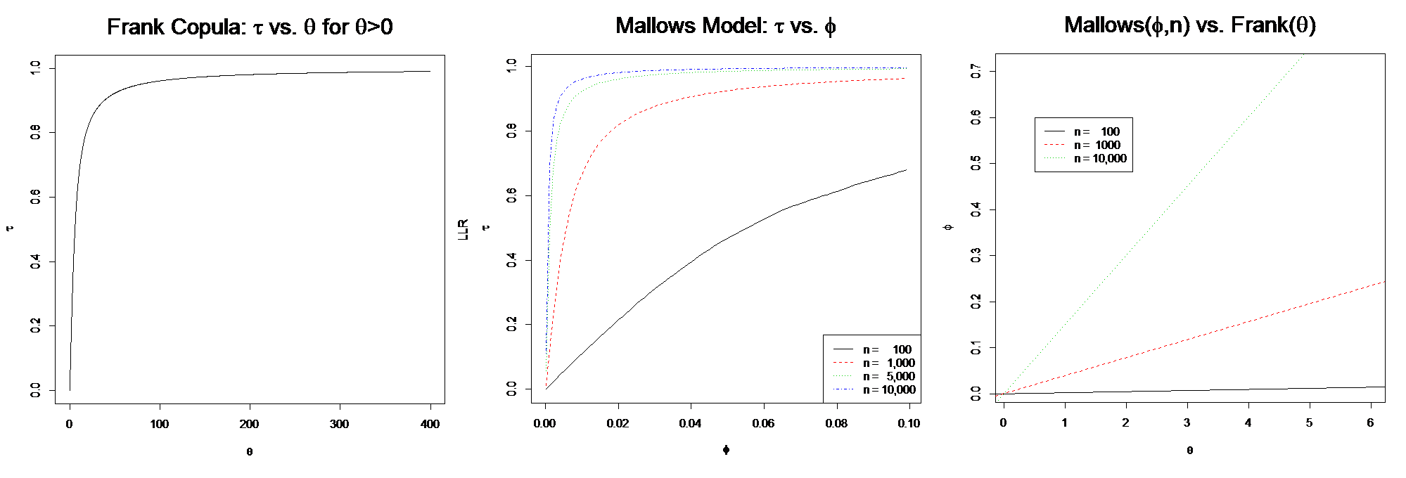
Figure 3. Scale relationships. Left: Kendall’s $\tau$ vs. the Frank scale $\theta$; Center: Kendall’s $\tau$ vs. the Mallows scale $\phi$ for $n=100,1000,5000,10000$; Right: Mallows $\phi_{n}$ vs. Frank$\theta$, for $n=100,1000,5000$.

Empirical evidence for the applicability of Proposition 4 comes in two stages: 1) The distribution of Kendall’s Distance under Frank$\left(\theta\right)$ and under Mallows$\left(\phi\left(\theta\right)\right)$ both converge to the same normal distribution; 2) As $n$ gets large the product density of the sample under Frank$\left(\theta\right)$ converges to an increasing function of the Kendall’s Distance between $\pi\left(\mathbf{X}\right)$ and $\nu\left(\mathbf{Y}\right)$ of the sample. Figure 4 illustrates results from the following confirmatory experiment:

• Generate 1000 sets of 1000 points from a Frank$\left(\theta=3\right)$ copula

• Compute the Kendall distance $D$ and the Frank density $d$ for each set

• Plot $d$ vs $D$ on a log-log scale

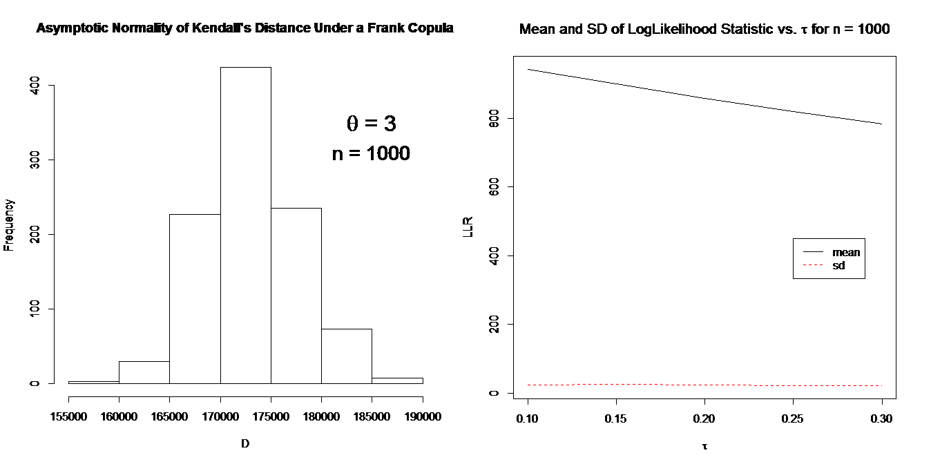
Figure 4. Association between $X$ and $Y$ in a Frank copula approaches a Mallows model for the ranking $\nu\left(\mathbf{Y}\right)$ in a large sample centered at $\pi\left(\mathbf{X}\right)$. Left: Approximate normality Kendall’s Distance $D$ in samples of size $n=1000$ from a Frank$\left(\theta=3\right)$ copula; Right: log-log plot of the density of each sample vs. its Kendall’s distance $D$.

Note also that the Frank copula is radially symmetric, $C\left(u,v\right)=u+v-1+C\left(1-u,1-v\right)$, which is a necessary condition for the density of a sample to depend only on its Kendall distance. With the assurance that there are copulas with the conditional distribution of $\nu\left(\mathbf{Y}\right)$ given $\pi\left(\mathbf{X}\right)$ well approximated by a Mallows model, this becomes the null hypothesis:

$$H_{0}:\nu\left(\mathbf{Y}\right)\circ\pi^{-1}\left(\mathbf{X}\right)\sim\textrm{Mallows}\left(\theta\right),\textrm{ for some }\theta>0.$$

The general alternative against which we would like a test to be sensitive is that there is a subpopulation with high association with the remainder having (little or) no association. The test for heterogeneity should maintain power over a wide variety of alternative distributions for the subpopulation supporting strong association. With these considerations, the alternative hypothesis is formulated as

$$H_{A}:\left(F\left(X\right),G\left(Y\right)\right)\sim M$$

where $M$ is a mixture of two distributions: $H_{1}$ on which $\left(F\left(X\right),G\left(Y\right)\right)$ are independent and $H_{2}$ on which $\left(F\left(X\right),G\left(Y\right)\right)$ have $\tau>0$.

To test against such a general alternative, an adaptive model encompassing the Mallows model is adopted, with the number of free parameters in the model increasing with sample size. This components of Kendall’s tau (CKT) test proceeds in four steps:

1. Fit a Mallows model centered at $\pi\left(\mathbf{X}\right)$ to $\nu\left(\mathbf{Y}\right)$ and compute the likelihood.

2. Reorder the data points $\left\{\left(X_{i},Y_{i}\right)\mid i=1,\ldots,n\right\}$, so that Kendall’s tau coefficient is decreasing. See Yu et al. (2011). Call the reordering $\sigma$.

3. Smoothly fit a multistage ranking model to the relative rankings of
   $\left[Y_{\sigma\left(1\right)},\ldots,Y_{\sigma\left(k\right)}\right]$ to $\left[X_{\sigma\left(1\right)},\ldots,X_{\sigma\left(k\right)}\right]$ at each stage $k$. See Sampath and Verducci (2013). Compute the likelihood under this (encompassing) model.

4. Use the (Generalized) Likelihood Ratio statistic to test $H_{0}$.

Comments on the four steps:

1. Since Kendall’s tau distance is invariant to reordering of observations, this is the same as fitting a Mallows model, centered at ranking $\left(\sigma X\right)$, to the ranking $\left(\sigma Y\right)$, where $\sigma$ is the taupath reordering.

2. The idea of reordering is to put the points displaying the highest amount of association earlier in the sequence in order to identify the subpopulation with highest empirical association. The reordering is not unique. Yu et al. (2011) discuss various algorithms.

3. The multistage ranking model decomposes the number of discordances [up to ($n$ choose 2)] between ranking $\left(\sigma Y\right)$ and ranking $\left(\sigma X\right)$, as a sum of $n-1$ variables $\left\{V_{k}\right\}$ with ranges $\left\{0,\ldots,k\right\}$, $k=1,\ldots,n-1$. The model has likelihood $L=c\left(\theta\right)e^{-\sum\theta_{k}V_{k}}$ which reduces to the likelihood of Mallows model when all component parameters are equal.

4. The conditions needed to justify an asymptotic chi-square distribution for this statistic do not hold in this setting. Currently, we simulate the distribution under the Frank copula to get an appropriate reference. We are working to find a more precise characterization of the LR in this setting.

The null distribution of this likelihood ratio appears to be close to normal, with its mean decreasing with the common correlation $\tau$, and standard deviation constant. See Figure 5. Note that, for $n=1000$, the variance of $2\cdot\textrm{LLR}\approx 2500$ is clearly less than its $2\cdot\textrm{mean$\left(2\cdot\textrm{LLR}\right)$}$ theoretical value for a chi square distribution, which is in the range $\left(3100,3800\right)$ when $\tau\in\left(.10,.30\right)$.

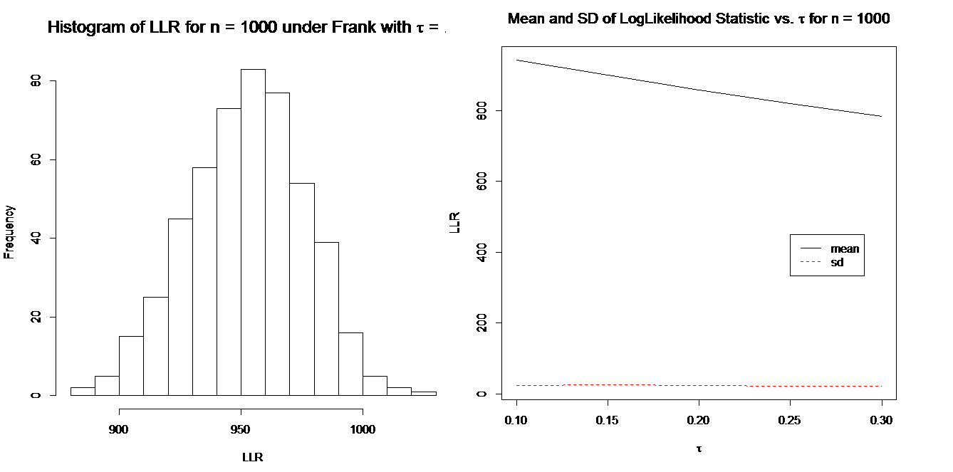
Figure 5. Simulation of Log Likelihood Ratio (LLR) Statistic for CKT test under Frank Copulas. Left: Histogram of $500$ simulations of size $n=1000$. Right: Decreasing pattern of mean and constancy of standard deviation for LLR under Frank Copulas at different levels of $\tau$ for $n=1000$.

Instead of fixed $n$ and varying $\tau$, Figure 6 depicts the relationship between LLR and $n$ with fixed $\tau=0.1$. The overall relationship between the moments of LLR and the parameters $\tau$ and $n$ is not yet known, but using a practical additive approximation in the range $.1<\tau<.3$ and $500<n<3000$, the basic asymptotic α-level CKT test has the form: Reject $H_{0}$ if

$$Z=\frac{\textrm{LLR}-\left(n+20-797\hat{\tau}\right)}{0.02n+7}>z_{1-\alpha},$$

where $\hat{\tau}$ is Kendall’s correlation coefficient and $z_{1-\alpha}$ is the $\left(1-\alpha\right)^{\textrm{th}}$ quantile of the standard normal.

Simulations for Robustness and Power

First, performance of the tests is checked by maintenance of levels under various Gaussian and Frank copulas; subsequently power is examined. The CSF test is based on the number of absolute rank differences less than .2. Figure 7 shows the null distributions of p-values for the CSF test applied to samples of size $n=1000$ generated 100,000 times under the Gaussian($\rho$) models. These distributions start to become stochastically smaller than uniform for $\rho>0.45$. Otherwise the test is conservative in the range $0<\rho<0.45$ and $0<\alpha<0.05$ as illustrated by the observed number of type 1 errors at the $\alpha=0.05$ level.

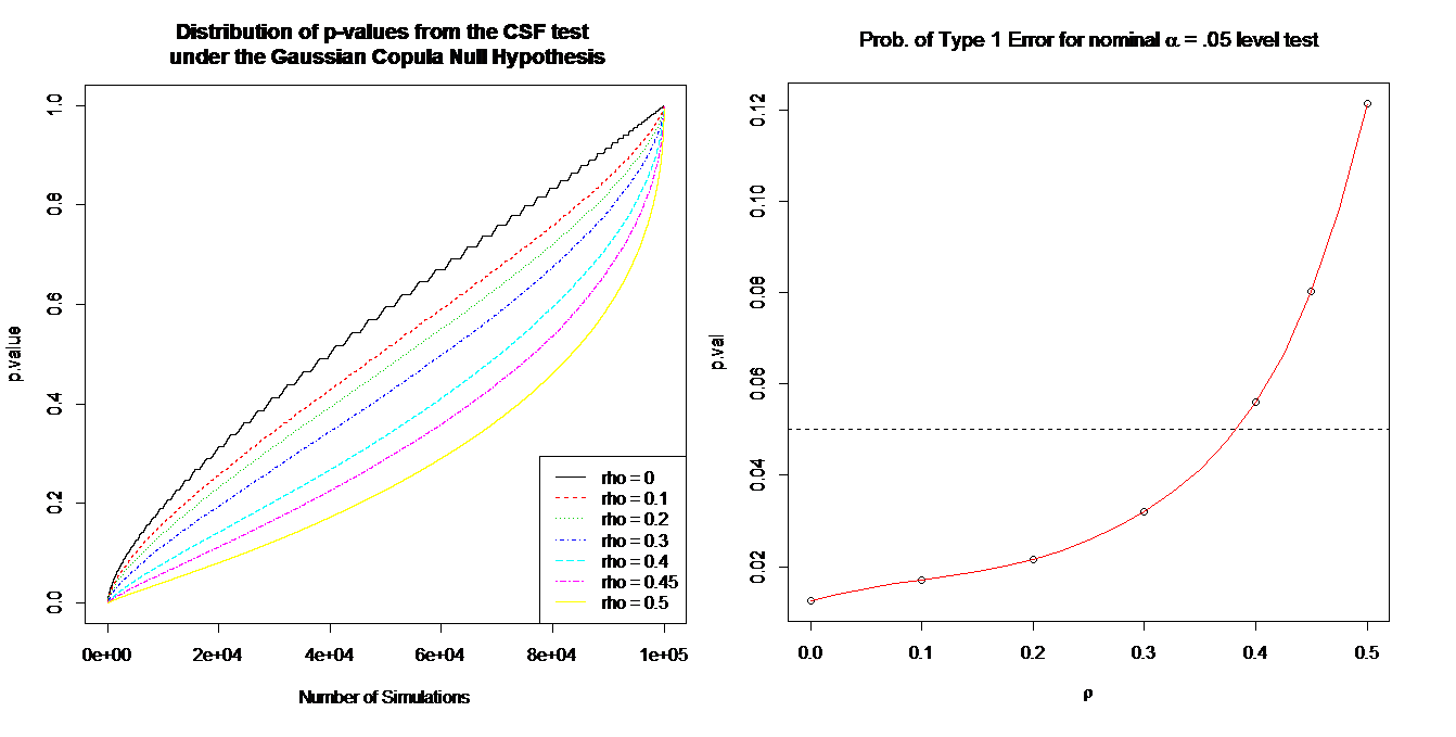
Figure 6. CSF results from $100,000$ simulation experiments of size $n=1000$ for values of $\rho$ in a Gaussian copula. Left: Distribution of p-values for 7 values of null correlation; Right: Observed probabilities of Type I error for a nominal $\alpha=0.05$ test. The test is conservative for values of $\rho<0.45$.

Under similar Gaussian copulas, the adjustment of the mean of the log-likelihood for the estimated overall $\tau$ makes the CKT test behave conservatively for large values of $\rho$, but gives highly significant values for $r$ values near 0. See Figure 8, in which, due to computational limitations, lowess-smoothed curves describe the p-distribution based on only 100 simulations. In the presence of very low overall correlation, it is advisable to use the CSF test as a screen for the CKT, which will protect the CKT from finding uneven levels of $\tau$ association when $\rho$ association is homogeneous. Again, this tendency toward excess false positives happens only when the overall $\rho$ association is close to 0. In this case a special test (Sampath and Verducci, 2013) is available for the null hypothesis of independence. Under a Frank copula, the CSF test behaves properly near independence, but loses its level when τ gets large. See Figure 9.

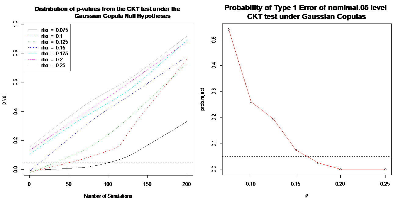
Figure 7. CKT results from 200 simulation experiments of size $n=1000$ for values of $\rho$ in a Gaussian copula; Left: Distribution of p-values for 7 values of the null correlation; Right: Obeserved probabilities of Type I error for a nominal $\alpha=0.05$ test. The test is conservative for values of $\rho>0.16$.

Several factors affect the power curves of both the CSF and CKT tests: sample size (n is fixed at 500 or 1000); proportionate size of the subpopulation (fixed at 40%); strength of association in the subpopulation $\left(\rho,\tau\in\left\{.7,.8,.9\right\}\right)$; and, most importantly, the form of the subpopulation. Against the null hypothesis of a Gaussian copula, the alternative is a mixture of copulas, where the variables are assumed to be independent in the complement of the subpopulation. Against the null hypothesis of a Frank discordancescopula, the subpopulation is selected at random and its conditional distribution is forced into a stronger Mallows model. This allows the population margins to remain uniform while possibly restricting the range of the subpopulation.

Figure 10 shows the distribution of p-values of both CSF and CKT tests against 40% Gaussian with $.12\leq\rho\leq.13$. For this range of overall correlation the CKT test holds its level and is conservative for overall correlation $\rho<.12$, which is the case here. Nevertheless, it achieves perfect power when the subpopulation $\rho\geq.125$, even though its power quickly diminishes to 10% for $\rho=.12$ in the subpopulation. It also performs better than CSF in this range.

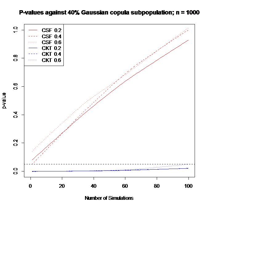
Figure 8. P-values against Alternative Mixture of Gaussian copulas with sample size $n=1000$ and subpopulation proportion $=40\%$. Dashed horizontal lines at $\alpha=0.05$ indicates the power of a level 0.05 test.

Under the Mallows alternative, $n=1000$ points are generated from a uniform distribution, 400 points are then sampled from a quantile range of x values and the y values resorted according to a random draw from a Mallow$\left(\phi\left(\tau\right)\right)$ model. Values of $\tau$ used are .4, .5, and .6. Figure 11 shows the distributions of p-values from the $\alpha=0.05$ level CSF and CKT tests over 100 simulations. The left panel corresponds to the subpopulation being sampled from the full range, while the right panel corresponds to samples between the 20th and 80th percentiles of x-values. The CKT test performs much better than the CSF test against these alternatives. The CKT has essentially perfect detection when the subpopulation spans the whole range, and at least 70% power in the 20-80 percentile range. The CSF has no power in either scenario.

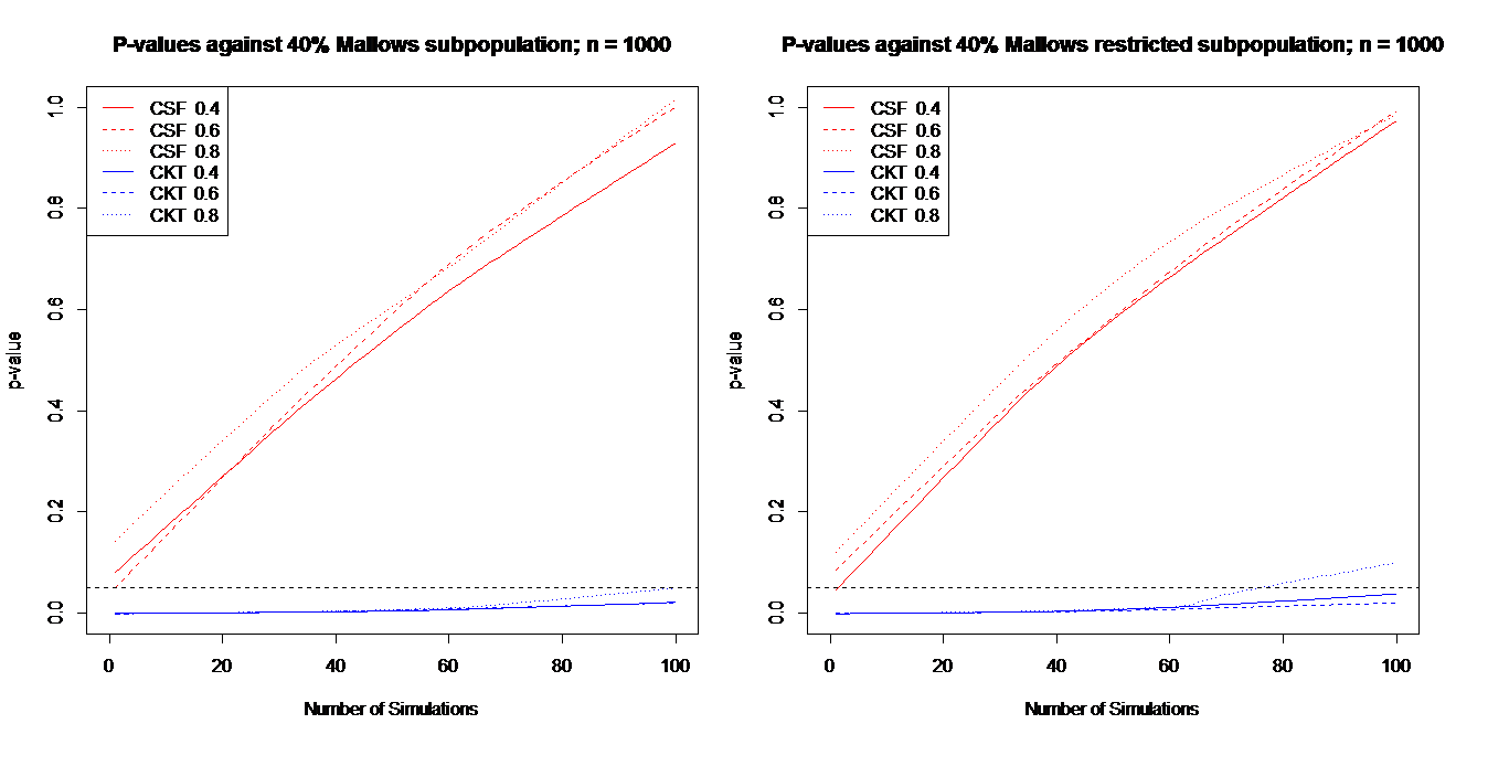
Figure 9. Distribution of p-values for Mallows alternatives, based on 100 simulations of sample size $n=1000$. Left: Associated subgroup spans the full range of x-values. Right: Span is restricted to the 20-to-80th percentiles region of x-values in the larger population.

Example

Wine cultivars are varieties of grapes that have been cultivated through selective breeding. Different varieties may be characterized by certain chemical properties of the wine they produce. Early work in supervised learning has been used to classify wine cultivars using chemical measurements of wine sample (Aeberhard, et al. 1993). These data, available at (http://archive.ics.uci.edu/ml/machine-learning-databases/wine), are reanalyzed here using the CKT and CSF tests as unsupervised methods of detecting different association structures that might help characterize different cultivated varieties.

Figure 12 shows the relationship between flavenoids and phenols in the data set consisting of 13 measurements from 178 wine samples derived from 3 different cultivars. To the untrained eye, the overall plot looks typical of homogeneous association, but both the CKT (p =.0002) and CSF (p=.027) indicate heterogeneity. Identification of cultivars in the plot shows separation of cultivar 1 and 3 samples from each other, with slightly negative association within each of these groups; however, their positioning contributes a kind of ecological correlation to the overall sample. In contrast, samples from cultivar 2 show a strong positive association between flavenoid and phenol content. This suggests an underlying genetic difference.

It is impressive that CKT can detect this heterogeneity of association from the unlabelled data, which looks like an overall positive association, part of which is ecological correlation. Although the CSF test does also indicate association, it is not as sensitive at detecting it in this situation, and its p-value would not present a strong case for heterogeneity if any correction is attempted for multiple comparisons over the 13 choose 2 (78) pairs of variables available.

Concluding Remarks

The ability to detect subpopulations that drive association has the potential of changing the way statistics are used to unveil structures in “Big Data.” Instead of employing extensive model searching with complex interaction, now relatively model-free methods are available to ascertain with precision is there is any simple mixture that better explains monotone association between variables. The CSF and CKT tests achieve this, either working together to screen and confirm or separately to find different forms of the subpopulation that most strongly supports the association.

These tests, however, are formally restricted to different forms of the meaning of “homogeneous association.” Strict legitimacy of the CSF test depends on the assumption of a Gaussian copula underlying the null distribution, whereas the CKT test depends on the assumption of a Frank copula underlying the null distribution. Although there is some evidence of limited robustness, much more work should be done to explore the behavior of these tests under general conditions. For example, both the Gaussian and Frank copulas are radially symmetric; it is unclear how sensitive the tests would be to asymmetric notions of homogeneous association.

The computationally efficiency of the CSF test is important because the sample size n needs to be in the thousands before there is much hope of reliably detecting these subtle but important differences. In contrast with the CSF test, the justification of CKT is a bit more compelling, based on intrinsic association within the subpopulation. We have been using CSF at a liberal $\alpha=0.05$ level as a screening devise to reduce the number of pairs of variables to be tested at a more stringent level.

Detecting heterogeneity of association is a difficult task. Such detection is practical only when the overall association is not too strong, the association in the subpopulation is strong, and the sample size is large. Nevertheless, such scenarios abound. We believe that these new methods will make Statistics ever more relevant in making good sense from Big Data.

References

- [1] Aeberhard S., Coomans D., and de Vel O. (1993). Improvements to the classification performance of RDA. Journal of Chemometrics 7 (2), 99-115.
- [2] Diaconis, P. and Graham, R.L. (1977). Spearman’s footrule as a measure of disarray. Journal of The Royal Statistical Society Series B - Statistical Methodology 39, 262-268.
- [3] Diaconis, P. and Ram, A. (2000). Analysis of systematic scan metropolis algorithms using Iwahori-Hecke algebra techniques. Michigan Math. J. 48, 157-190.
- [4] Frank, M.J. (1979). On the simultaneous associativity of F(x, y) and x + y − F(x, y). Aequationes Mathematicae 19, 194-226.
- [5] Fermanian J.D., Radulovic D. and Wegkamp M. (2004). Weak convergence of empirical copula processes. Bernoulli 10, 847–860.
- [6] Genest, C. (1987). Frank’s family of bivariate distributions. Biometrika 74(3), 549–555.
- [7] Genest, C. and MacKay, J. (1986). The Joy of Copulas: Bivariate Distributions with Uniform Marginals. American Statistician 40, 280-283.
- [8] Genest, C. and Nešlehová, J. (2014). On tests of radial symmetry for bivariate copulas. Statistical Papers, 55.
- [9] Katz, G. (2014). How much do we know about HDL cholesterol? Clinical Correlations (http://www.clinicalcorrelations.org/?p=7298)
- [10] Lehmann, E.L. and Romano, J.P. (2006). Testing Statistical Hypotheses, 3rd Edition. Springer: New York.
- [11] Nelsen, R.B. (2006). An Introduction to Copulas, 2nd Edition. Springer:New York.
- [12] Sampath, S. and Verducci, J. (2013) Detecting the end of agreement between two long ranked lists. Statistical Analysis and Data Mining, 6 (6), 458–471.
- [13] Sen, P.K., Salama I.A. and Quade, D. (2011) Spearman’s Footrule: Asymptotics in Applications. Chilean Journal of Statistics, 2, 3:20.
- [14] Starr, Shannon (2009). Thermodynamic Limit for the Mallows Model on . J. Math. Phys. 50 195-208
- [15] Voight, B. F. et al. (2012) Plasma HDL cholesterol and risk of myocardial infarction: a mendelian randomisation study. The Lancet, 380 (9841), 572-580.
- [16] Yu, L., Verducci, J. and Blower, P. (2011) The Tau-Path Test for Monotone Association in an Unspecified Subpopulation: Applications to Chemogenomic Data Mining,” Statistical Methodology 8, 97-111.