Abstract

In contrast to the optomechanically induced transparency (OMIT) defined conventionally, the inverse OMIT behaves as coherent absorption of the input lights in the optomechanical systems. We characterize a feasible inverse OMIT in a multi-channel fashion with a double-sided optomechanical cavity system coupled to a nearby charged nanomechanical resonator via Coulomb interaction, where two counter-propagating probe lights can be absorbed via one of the channels or even via three channels simultaneously with the assistance of a strong pump light. Under realistic conditions, we demonstrate the experimental feasibility of our model by considering two slightly different nanomechanical resonators and the possibility of detecting the energy dissipation of the system. In particular, we find that our model turns to be a unilateral inverse OMIT once the two probe lights are different with a relative phase, and in this case the relative phase can be detected precisely.

OCIS codes: (270.0270) Quantum optics; (220.4880) Optomechanics; (270.1670) Coherent optical effects; (140.3948) Microcavity devices.

1 Introduction

Electromagnetically induced transparency (EIT) [1] is caused by quantum interference, creating a narrow transmission window within an absorption line. EIT was first theoretically predicted in three-level atoms [2, 3, 4, 5, 6, 7, 8] and then observed in optically opaque strontium vapor [9, 10]. So far, EIT effects have attracted considerable attention both theoretically and experimentally due to relevant optical effects and applications, such as, optical Kerr effect and optical switch [11, 12], slow light and quantum memory [13, 14, 15], and quantum interference and vibrational cooling [16, 17]. The key point in realization of the EIT effect is to find a $\Lambda$-type level configuration and construct quantum interference. In this context, for some hybrid systems with $\Lambda$-type level structures, e.g., metal materials [18], coupled waveguides [19, 20, 21], atom-cavity systems [22], and optomechanical systems [23, 24, 25, 26, 27, 28, 29, 30, 31, 32, 33], the analog of the EIT effects can also be observed.

The analog of the EIT effects in the optomechanics is named as the optomechanically induced transparency (OMIT), which was predicted in a pioneering theoretical work [32], and then verified experimentally [20, 34]. Very recently, not only the slow light was experimentally confirmed in the OMIT system [35], but also the optomechanical dark mode was observed experimentally [36]. Motivated by these experiments, many different proposals [33, 37, 38, 39, 40, 41, 42, 43, 44, 45, 46] were proposed based on the OMIT effect. One of the outstanding works is for an inverse OMIT [44] in an optomechanical cavity, i.e., an optomechanical resonator inside a single-mode cavity, which shows that, when two weak counter-propagating probe lights within the narrow transmission window of the OMIT are injected simultaneously, neither of the probe lights can be output from the cavity due to complete absorption by the optomechanics. Therefore, this effect is also named to be the coherent perfect absorption and has been stretched to two optomechanical cavities coupled to an optomechanical resonator [45], showing the prospective for coherent perfect transmission and beyond. However, both the schemes [44, 45] are very hard to achieve experimentally due to stringent conditions involved. As a result, it is desirable to have an experimentally feasible scheme for demonstrating the inverse OMIT. In addition, exploring the applications of the inverse OMIT is also interesting and experimentally demanded.

On the other hand, with an optomechanical cavity coupled to an external nanomechanical resonator (NR) via Coulomb interaction, the single narrow transmission window in the output light is split into two narrower transmission windows with the splitting governed by the Coulomb coupling [46]. This is due to the fact that an additional hybrid energy level is introduced into the original three-level system by the Coulomb coupling between the external NR and the optomechanical resonator. Similar double OMIT effect can also be observed when the optomechanical resonator interacts with a qubit [47] or an NR [48, 49, 50]. The Coulomb interaction works for a wide range from nanometer to meter [46, 51, 52] and can be controlled by the bias voltage [46, 52]. Besides, it can also be applied to different kinds of charged objects at different frequencies [51]. These advantages remind us of the necessity to explore a multi-channel inverse OMIT in the optomechanical system with the tunable Coulomb interaction.

In the present work, by considering a double-sided optomechanical cavity (involving a charged NR) coupled to another identical charged NR nearby via Coulomb interaction, we present a multi-channel inverse OMIT and study the energy dissipation of the system through the intracavity photon number and the mechanical excitations of the NRs. In addition, we explore a unilateral inverse OMIT, i.e., observation of the inverse OMIT available only on one side of the optomechanical cavity. Our study shows that this unilateral inverse OMIT could be applied to precision measurement of the relative phase between two probe lights.

Compared with previous studies, our idea includes more interesting physics and thus owns different applications. First, our inverse OMIT is generated from a double-OMIT system. It is a multi-channel inverse OMIT with the windows of narrower profiles than the counterpart in [44, 45], and the dissipation of the input probe light can be directly detected by the external NR, without the need of an additional light field as required in [44, 45]. Second, if there is a relative phase between two probe lights, the inverse OMIT is observed only on one side of the optomechanical cavity, which is essentially different from the inverse OMIT in [44, 45]. This unilateral inverse OMIT can not only reduce the experimental difficulty for demonstrating the inverse OMIT effects, but also be very sensitive to the relative phase between the two probe lights. As such, it can be applied to detect the relative phase between two probe lights. In addition, different from the analog of electromagnetically induced absorptions realized by a Stokes process in the region of blue detuning [35, 53], our scheme can be achieved by an anti-Stokes process in the region of red detuning. We argue below that these characteristics might be helpful for practical applications using optomechanical systems.

The present paper is structured as follows. Sec. 2 presents the model and an analytical solution to the multi-channel inverse OMIT of an optomechanical system. In Sec. 3, we characterize the output probe fields. Under some realistic conditions, we explore in Sec. 4 the situation of non-identical NRs, the energy dissipation and a possible application in precision measurement. The experimental feasibility is discussed in Sec. 5. A brief conclusion can be found in the last section.

2 The model and solution

Fig. 1: Schematic diagram for a double-sided cavity with a nanomechanical resonator NR₁ located at the node of the cavity mode and a nanomechanical resonator NR₂ outside. NR₁ is charged by the bias gate voltage $V_{1}$ and subject to the Coulomb force due to another charged NR₂ with the bias gate voltage $V_{2}$. The optomechanical cavity of length $L$ is driven by three light fields, one of which is the pump field $\varepsilon_{c}$ with frequency $\omega_{c}$ and the other of which are the probe fields $\varepsilon_{L(R)}$ with frequency $\omega_{p}$. The output field is represented by $\varepsilon_{outL(R)}$. $q_{1}$ and $q_{2}$ represent the small displacements of NR₁ and NR₂ from their equilibrium positions, and $r_{0}$ is the equilibrium distance between the two charged NRs.

As sketched in Fig. 1, our system consists of a Fabry-Perot (FP) cavity and two charged NRs, i.e., NR₁ and NR₂. The NR₁ is inside the FP cavity formed by two fixed mirrors with finite equal transmissions, and couples to the cavity mode with a radiation pressure. The NR₁ also interacts with the NR₂ outside the FP cavity via a tunable Coulomb interaction. We suppose that the FP cavity is driven by a strong pump field (frequency $\omega_{c}$) from the left-hand side of the cavity, and two weak classical probe fields (frequency $\omega_{p}$) are injected into the cavity from both sides of the cavity. The Hamiltonian in the rotating frame at the pump field frequency $\omega_{c}$ can be written as [46, 48]

$$H = \hbar(\omega_{0}-\omega_{c})c^{{\dagger}}c+(\frac{p_{1}^{2}}{2m_{1}}+\frac{1}{2}m_{1}\omega_{1}^{2}q_{1}^{2})+(\frac{p_{2}^{2}}{2m_{2}}+\frac{1}{2}m_{2}\omega_{2}^{2}q_{2}^{2})+i\hbar\varepsilon_{c}(c^{{\dagger}}-c)$$ (1)

$$+ i\hbar(c^{{\dagger}}\varepsilon_{L}e^{-i\delta t}-h.c.)+i\hbar(c^{{\dagger}}\varepsilon_{R}e^{-i\delta t}-h.c.)+\hbar g_{0}c^{{\dagger}}cq_{1}+\hbar\lambda_{0}q_{1}q_{2},$$

where the first three terms represent the free parts of the Hamiltonian for the cavity field and the NRs. $c\ (c^{{\dagger}})$ is the annihilation (creation) operator of the cavity mode at frequency $\omega_{0}$. The charged NR₁ (NR₂) owns the frequency $\omega_{1}$ ($\omega_{2}$), the effective mass $m_{1}$ ($m_{2}$), the position $q_{1}$ ($q_{2}$) and the momentum $p_{1}$ ($p_{2}$) [41]. The next three terms describe the cavity mode driven by a pump field and two probe fields. $\varepsilon_{c}=\sqrt{2\kappa\wp_{c}/\hbar\omega_{c}}$ ($\varepsilon_{L(R)}=\sqrt{2\kappa\wp_{p}/\hbar\omega_{p}}$) is an amplitude of the strong pump (weak probe) field with $\wp_{c}$ ($\wp_{p}$) and $\kappa$ being the power of the pump (probe) field and the cavity decay rate, respectively, and $\delta=\omega_{p}-\omega_{c}$ is a detuning between the probe field and the pump field. The last two terms include the coupling of the NR₁ to the cavity mode via the radiation pressure strength $g_{0}$ [54], and also the interaction between the NR₁ and NR₂ with the Coulomb coupling strength $\lambda_{0}=\frac{C_{1}V_{1}C_{2}V_{2}}{2\pi\hbar\varepsilon_{0}r_{0}^{3}}$[51, 55]. The NR₁ (NR₂) takes the charge $Q_{1}=C_{1}V_{1}$ ($Q_{2}=-C_{2}V_{2}$), with $C_{1}(C_{2})$ and $V_{1}(-V_{2})$ being the capacitance and the voltage of the bias gate, respectively.

With the annihilation (creation) operator $b_{j}$ ($b_{j}^{\dagger}$), the position and momentum operators of the NR_j are rewritten as $q_{j}=\sqrt{\frac{\hbar}{2m_{j}\omega_{j}}}(b_{j}+b_{j}^{\dagger})$, and $p_{j}=i\sqrt{\frac{\hbar m_{j}\omega_{j}}{2}}(b_{j}^{\dagger}-b_{j})$, which yields the Hamiltonian

$$H^{\prime}=\hbar\Delta_{c}c^{{\dagger}}c+\hbar\omega_{1}b_{1}^{\dagger}b_{1}+\hbar\omega_{2}b_{2}^{\dagger}b_{2}$$

$$+\hbar gc^{{\dagger}}c(b_{1}+b_{1}^{\dagger})+i\hbar\varepsilon_{c}(c^{{\dagger}}-c)+\hbar\lambda(b_{1}^{\dagger}+b_{1})(b_{2}^{\dagger}+b_{2})$$

$$+i\hbar(c^{{\dagger}}\varepsilon_{L}e^{-i\delta t}-h.c.)+i\hbar(c^{{\dagger}}\varepsilon_{R}e^{-i\delta t}-h.c.),$$ (2)

with $\Delta_{c}=\omega_{0}-\omega_{c}$, $g=g_{0}\sqrt{\hbar/2m_{1}\omega_{1}}$ and $\lambda=\frac{\hbar\lambda_{0}}{2}\sqrt{m_{1}m_{2}\omega_{1}\omega_{2}}$.

Considering the damping and noise terms, the quantum Langevin equations are generated from Eq. (2),

$$\begin{array}[]{ccl}\dot{b_{1}}&=&-(\frac{\gamma_{1}}{2}+i\omega_{1})b_{1}-igc^{{\dagger}}c-i\lambda(b_{2}^{\dagger}+b_{2})+\sqrt{\gamma_{1}}b_{1}^{in},\\ \dot{b_{2}}&=&-(\frac{\gamma_{2}}{2}+i\omega_{2})b_{2}-i\lambda(b_{1}^{\dagger}+b_{1})+\sqrt{\gamma_{2}}b_{2}^{in},\\ \dot{c}&=&-(2\kappa+i\Delta_{c})c-ig(b_{1}+b_{1}^{{\dagger}})c+\varepsilon_{c}+(\varepsilon_{L}+\varepsilon_{R})e^{-i\delta t}+\sqrt{2\kappa}(c_{in}+d_{in}),\end{array}$$ (3)

where $\gamma_{1}$ ($\gamma_{2}$) is the NR₁ (NR₂) decay rate, $2\kappa$ is the cavity decay rate from the two sides. The quantum Brownian noise $b_{1}^{in}$ $(b_{2}^{in})$ is resulted from the coupling between the NR₁ (NR₂) and the environment [56]. $c_{in}(d_{in})$ is the input quantum noise from the environment [56]. The mean values of the noise terms $b_{1}^{in}$, $b_{2}^{in}$, $c_{in}$, and $d_{in}$ are zero.

Equation (3) is solved under the conditions: (i) The sideband resolved regime ($\omega_{1}\gg\kappa$); (ii) $\delta\simeq\omega_{1}$ and $\delta\simeq\omega_{2}$; (iii) $\Delta\sim\omega_{1}$. The first condition ensures an observable normal mode splitting due to strong coupling between the NR₁ and the cavity mode; The second condition yields $\delta^{2}-\omega_{1}^{2}=2\omega_{1}(\delta-\omega_{1})$ and $\delta^{2}-\omega_{2}^{2}=2\omega_{2}(\delta-\omega_{1})$; The last one is to eliminate the detuning $\Delta$. We also suppose that each operator is a mean value plus a small quantum fluctuation, i.e., $o=o_{s}+\delta o$, with $o=b_{1}$, $b_{2}$, and $c$, and $\delta o\ll|o_{s}|$. Inserting them into Eq. (3) and neglecting the second-order smaller terms, we obtain the steady-state mean values of the system as

$$\begin{array}[]{lll}b_{1s}&=\frac{-ig|c_{s}|^{2}}{\frac{\gamma_{1}}{2}+i\omega_{1}+\frac{8\lambda^{2}\omega_{1}\omega_{2}}{(\omega_{1}+i\frac{\gamma_{1}}{2})(\omega_{2}+i\frac{\gamma_{2}}{2})(\frac{\gamma_{2}}{2}+i\omega_{2})}}&\simeq\frac{-ig|c_{s}|^{2}}{\frac{\gamma_{1}}{2}+i\omega_{1}+\frac{8\lambda^{2}}{\frac{\gamma_{2}}{2}+i\omega_{2}}},\\ b_{2s}&=\frac{-2\lambda\omega_{1}}{(\omega_{1}+i\frac{\gamma_{1}}{2})(\omega_{2}-i\frac{\gamma_{2}}{2})}\simeq\frac{-i2\lambda}{\frac{\gamma_{2}}{2}+i\omega_{2}}b_{1s},&c_{s}=\frac{\varepsilon_{c}}{2\kappa+i\Delta}\end{array}$$ (4)

with $\Delta=\omega_{0}-\omega_{c}+g(b_{1s}+b_{1s}^{\ast})$, and the corresponding linearized quantum Langevin equations for the small quantum fluctuations are of the form

$$\begin{array}[]{ccl}\dot{\delta b}_{1}&=&-({\frac{{\gamma_{1}}}{2}+}i{\omega_{1}})\delta{b_{1}}-i({G^{\ast}\delta c+G\delta c^{\dagger})}-i\lambda(\delta{b_{2}+}\delta b_{2}^{\dagger})+\sqrt{{\gamma_{1}}}b_{1}^{in},\\ \dot{\delta b}_{2}&=&-(\frac{{\gamma_{2}}}{2}+i{\omega_{2}})\delta{b_{2}}-i\lambda(\delta{b_{1}+}\delta b_{1}^{\dagger})+\sqrt{{\gamma_{2}}}b_{2}^{in},\\ \dot{\delta c}&=&-(2\kappa+i\Delta)\delta c-iG(\delta{b_{1}}+\delta b_{1}^{\dagger})+({\varepsilon_{L}}+{\varepsilon_{R}}){e^{-i\delta t}}+\sqrt{2\kappa}({c_{in}}+{d_{in}}),\end{array}$$ (5)

with $G=gc_{s}$ being the effective radiation pressure coupling.

The inverse OMIT effect can be studied by analyzing the mean response of the system to two probe fields in the presence of the pump field. After input noises of the system are ignored, the mean value equations with the probe fields in Eq. (5) are rewritten as [32, 33]

$$\begin{array}[]{ccl}\langle\dot{\delta b}_{1}\rangle&=&-i({G^{\ast}}\left\langle{\delta c}\right\rangle{+G}\left\langle{\delta c^{\dagger}}\right\rangle{)}-(i{\omega_{1}+\frac{{\gamma_{1}}}{2}})\langle\delta{b_{1}}\rangle-i\lambda(\langle\delta{b_{2}}\rangle+\langle\delta b_{2}^{\dagger}\rangle),\\ \langle\dot{\delta b}_{2}\rangle&=&-(i{\omega_{2}}+\frac{{\gamma_{2}}}{2})\langle\delta{b_{2}}\rangle-i\lambda(\langle\delta{b_{1}}\rangle+\langle\delta b_{1}^{\dagger}\rangle),\\ \langle\dot{\delta c}\rangle&=&-(2\kappa+i\Delta)\langle\delta c\rangle-iG(\langle\delta{b_{1}}\rangle+\langle\delta b_{1}^{\dagger}\rangle)+({\varepsilon_{L}}+{\varepsilon_{R}}){e^{-i\delta t}}.\end{array}$$ (6)

Define the solution to Eq. (6) takes the following form [33]

$$\langle\delta o\rangle=\delta o_{+}e^{-i\delta t}+\delta{o}_{-}e^{i\delta t},$$ (7)

the results for the small quantum fluctuations is given by

$$\begin{array}[]{ccl}\delta b_{1+}&=&\frac{-iG^{\ast}}{\frac{{\gamma_{1}}}{2}-i(\delta-{\omega_{1}})+\frac{{\lambda^{2}}}{{\frac{{\gamma_{2}}}{2}}-i(\delta-{\omega_{2}})}}\delta c_{+},\\ \delta b_{2+}&=&\frac{-i\lambda}{\frac{\gamma_{2}}{2}+i\omega-i\delta}\delta b_{1+},\\ \delta c_{+}&=&\frac{\varepsilon_{L}+\varepsilon_{R}}{2\kappa+i(\Delta-\delta)+\frac{|G|^{2}}{A}},\end{array}$$ (8)

with $A=\frac{{\gamma_{1}}}{2}-i(\delta-\omega_{1})+\frac{{\lambda^{2}}}{{\frac{{\gamma_{2}}}{2}}-i(\delta-{\omega_{2}})}$. Our scheme includes a more general situation than in [44] since our results can be reduced to the counterpart in [44] in the absence of the Coulomb coupling. It is confirmed in the comparison with the output field involving two tunable central frequencies for the inverse OMIT in [44] that our scheme owns three frequencies for the inverse OMIT effect, two of which can be adjusted by the Coulomb interaction.

3 The inverse OMIT

Based on the solutions above, we present below the multi-channel inverse OMIT in our system with some channels controllable by the driven field due to effective coupling and Coulomb interaction between the NRs.

For simplicity, we first assume two identical charged NRs ($\omega_{1}=\omega_{2}=\omega_{m}$) and the detuning between the pump field and the cavity mode satisfying $\Delta\simeq\omega_{m}$. This assumption helps an analytical understanding of characteristics of the model, but changes nothing in the physical essence of the considered system. The assumption will be released later under consideration of realistic condition.

Considering the output fields from the two sides of the cavity by the input-output relations [57]

$$\varepsilon_{out\alpha}+\varepsilon_{\alpha}e^{-iDt}=2\kappa\langle\delta c\rangle,~{}~{}~{}\alpha=R,L,$$ (9)

with $D=\delta-\omega_{m}$, we define the output fields as

$$\varepsilon_{out\alpha}=\varepsilon_{out\alpha+}e^{-iDt}+\varepsilon_{out\alpha-}e^{iDt},~{}~{}~{}\alpha=R,L,$$ (10)

where $\varepsilon_{out\alpha+}$ and $\varepsilon_{out\alpha-}$ are the responses at the frequencies $\omega_{p}$ and $2\omega_{c}-\omega_{p}$ in the original frame.

Using Eqs. (7), (9) and (10), the output fields at the probe frequency $\omega_{p}$ are presented as

$$\begin{array}[]{rl}\varepsilon_{out\alpha+}=&2\kappa\delta{c}_{+}-\varepsilon_{\alpha}\\ =&\frac{\varepsilon_{L}+\varepsilon_{R}}{2\kappa+iD+\frac{|G|^{2}}{\frac{{\gamma_{1}}}{2}-i(\delta-\omega_{1})+\frac{{\lambda^{2}}}{{\frac{{\ \gamma_{2}}}{2}}-iD}}}-\varepsilon_{\alpha}\end{array}~{}~{}~{}$$ (11)

with $\alpha=R,L$.

The zero output fields, i.e., $\varepsilon_{outR+}=\varepsilon_{outL+}=0,$ occur under the following conditions

$$\varepsilon_{L}=\varepsilon_{R},\gamma_{1}=\gamma_{2}=2\kappa,\lambda^{2}=\frac{1}{2}|G|^{2}-\kappa^{2}.$$ (12)

Thus there are three channels at

$$D_{0} = 0,$$

$$D_{\pm} = \pm\sqrt{|G|^{2}+\lambda^{2}-3\kappa^{2}}=\pm\sqrt{\frac{3}{2}|G|^{2}-4\kappa^{2}},$$ (13)

for the coherent perfect absorption, implying that the probe lights cannot be reflected or transmitted from this optomechanical system, but entirely absorbed. This is due to a perfect destructive interference between the two probe lights along opposite directions. The energy of the probe lights will be finally dissipated via the vibrational decay of the NRs and the thermal-photon decay in the optomechanics, as discussed in detail later. As a result, this optomechanical system can be used to realize the multi-channel inverse OMIT (Fig. 2) with the essential prerequisite of the optomechanical normal-mode splitting [44].

For the detuning cases of $D_{\pm}=\pm\sqrt{\frac{3}{2}|G|^{2}-4\kappa^{2}}$, the effective coupling rate should follow $|G|\geq\sqrt{\frac{8}{3}}\kappa$. $D_{0}=D_{\pm}=0$ is a special case representing only a single channel involved in the inverse OMIT when $|G|=\sqrt{\frac{8}{3}}\kappa$ and $\lambda=\frac{1}{\sqrt{3}}\kappa$. Considering the general cases with $|G|>\sqrt{\frac{8}{3}}\kappa$, there are three channels as presented in Eq. (13), corresponding to the three injected probe lights at the frequencies $\omega_{p}=\omega_{c}+\omega_{m}$ and $\omega_{p}=\omega_{c}+\omega_{m}+D_{\pm}$ with $D_{\pm}=\pm\sqrt{\frac{3}{2}|G|^{2}-4\kappa^{2}}$. For example, in the case of $|G|=2\kappa$ and $\lambda=\kappa$, the inverse OMIT effect can be observed at $D_{0}=0$ and $D_{\pm}=\pm\sqrt{2}\kappa$, corresponding to the three injected probe lights at the frequencies $\omega_{p}=\omega_{c}+\omega_{m}$ and $\omega_{p}=\omega_{c}+\omega_{m}\pm\sqrt{2}\kappa$, respectively. Moreover, these two additional windows become more separate with the increase of both the effective radiation coupling $|G|$ and the corresponding Coulomb coupling $\lambda=\sqrt{\frac{1}{2}|G|^{2}-\kappa^{2}}$, as demonstrated in Fig. 2.

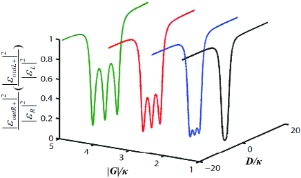
Fig. 2: The normalized output probe photon number $|\frac{\varepsilon_{outR+}}{\varepsilon_{L}}|^{2}$ $(|\frac{\varepsilon_{outL+}}{\varepsilon_{L}}|^{2})$ as functions of the probe detuning $D/\kappa$ and the effective radiation coupling $|G|/\kappa$, where $D=\omega_{p}-\omega_{c}-\omega_{m}$.

4 Discussion

4.1 Multi-channel inverse OMIT with two non-identical NRs

The two identical NRs considered above are theoretically simplified, but rarely existing experimentally. To release this stringent condition, we consider below the multi-channel inverse OMIT with non-identical NRs.

For two charged NRs with different frequencies, as plotted in Fig. 3 , the multi-channel inverse OMIT occurs with some window shifts with respect to the case of identical NRs, turning it to be asymmetric for the curves of the normalized probe photon number versus the probe detuning. It can be understood from the bright mechanical mode $b=b_{2}\sin\theta+b_{1}\cos\theta$ and the dark one $d=b_{2}\cos\theta-b_{1}\sin\theta$ with $\tan\theta=[(\omega_{2}-\omega_{1})+\sqrt{4\lambda^{2}+(\omega_{2}-\omega_{1})^{2}}]/(2\lambda)$, which are the diagonalized orthogonal modes of the two coupled mechanical modes $b_{1}$ and $b_{2}$. These bright and dark modes can effectively couple to the optical mode with the strengths $|G|\cos\theta$ and $|G|\sin\theta$, respectively. In contrast to the case of $\omega_{1}=\omega_{2}$ with both the bright and dark modes sharing the same coupling strength $|G|/\sqrt{2}$, the effective couplings for the bright and dark modes are different in the case of $\omega_{1}\neq\omega_{2}$. Different from the symmetric curves in the case of $\omega_{1}=\omega_{2}$, the curves of the normalized probe photon number versus the probe detuning move leftward if $\omega_{1}>\omega_{2}$ and rightward if $\omega_{1}<\omega_{2}$ (see Fig. 3). This implies that the middle channel of this multi-channel inverse OMIT is not always fixed, but variable if we appropriately tune the frequencies of the NRs, as in [58].

More differences can be found in the discussion below from the comparison between the identical and non-identical NRs.

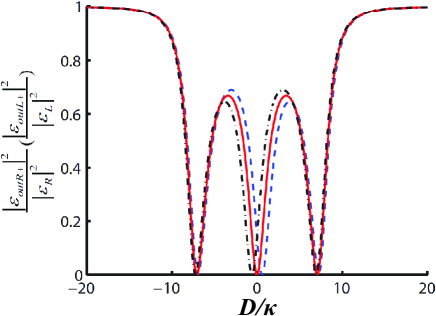
Fig. 3: The normalized output probe photon number $|\frac{\varepsilon_{outR+}}{\varepsilon_{R}}|^{2}$ $(|\frac{\varepsilon_{outL+}}{\varepsilon_{L}}|^{2})$ as a function of the probe detuning $D/\kappa$, where $D=\omega_{p}-\omega_{c}-\omega_{m}$ for identical NRs and $D=\omega_{p}-\omega_{c}-\omega_{1}$ for non-identical case. The red solid, black dashed-dotted, and blue dashed curves are for $\omega_{2}=\omega_{1}$, $\omega_{2}=0.8\omega_{1}$ and $\omega_{2}=1.2\omega_{1}$, respectively, if $|G|=6\kappa$.

Table 1: The relationship among the normalized output probe photon numbers ($\varepsilon_{outR+}$ and $\varepsilon_{outL+}$), the intracavity probe photon numbers ($\frac{4\kappa^{2}}{|\varepsilon_{L}|^{2}+|\varepsilon_{R}|^{2}}|\delta c_{+}|^{2}$), and the mechanical excitations ($\frac{4\kappa^{2}}{|\varepsilon_{L}|^{2}+|\varepsilon_{R}|^{2}}|\delta b_{1+}|^{2}$, $\frac{4\kappa^{2}}{|\varepsilon_{L}|^{2}+|\varepsilon_{R}|^{2}}|\delta b_{2+}|^{2}$ and the summation) for different effective radiation $|G|$ and Coulomb coupling strengths $\lambda$ in the inverse OMIT. Part I presents the middle channel $D=D_{0}$ and part II for the side channels $D=D_{\pm}$. We consider two non-identical NRs with $\omega_{1}=1.2\kappa$ and $\omega_{2}=\kappa$ and the identical case with $\omega_{1}=\omega_{2}=\kappa$. The values in parentheses are for the identical case.

	$D/\kappa$	$|G|/\kappa$	$\lambda/\kappa$	$\varepsilon_{outR+}$	$\varepsilon_{outL+}$	$\frac{4\kappa^{2}}{|\varepsilon_{L}|^{2}+|\varepsilon_{R}|^{2}}|\delta c_{+}|^{2}$	$\frac{4\kappa^{2}}{|\varepsilon_{L}|^{2}+|\varepsilon_{R}|^{2}}|\delta b_{1+}|^{2}$	$\frac{4\kappa^{2}}{|\varepsilon_{L}|^{2}+|\varepsilon_{R}|^{2}}|\delta b_{2+}|^{2}$	$\frac{4\kappa^{2}}{|\varepsilon_{L}|^{2}+|\varepsilon_{R}|^{2}}(|\delta b_{1+}|^{2}+|\delta b_{2+}|^{2})$
	0.198 (0)	$2$	$1$			0.503 (0.5)	0.4985 (0.5)	0.4985 (0.5)	0.997(1.0)
I	0.140 (0)	$4$	$\sqrt{7}$	0 (0)	0 (0)	0.501 (0.5)	0.125(0.125)	0.874(0.875)	0.999(1.0)
	0.136 (0)	$6$	$\sqrt{17}$			0.518 (0.5)	0.006(0.056)	0.976(0.944)	0.982(1.0)
	$\begin{array}[]{c}+1.417\\ -1.415\end{array}$($\pm\sqrt{2}$)	$2$	$1$			$\begin{array}[]{c}0.502\\ 0.500\end{array}$(0.5)	$\begin{array}[]{c}0.711\\ 0.783\end{array}$(0.75)	$\begin{array}[]{c}0.287\\ 0.217\end{array}$(0.25)	$\begin{array}[]{c}0.998\\ 1.000\end{array}$(1.0)
II	$\begin{array}[]{c}+4.629\\ -4.358\end{array}$($\pm 2\sqrt{5}$)	$4$	$\sqrt{7}$	0 (0)	0 (0)	$\begin{array}[]{c}0.492\\ 0.508\end{array}$(0.5)	$\begin{array}[]{c}0.742\\ 0.757\end{array}$(0.75)	$\begin{array}[]{c}0.266\\ 0.235\end{array}$(0.25)	$\begin{array}[]{c}1.008\\ 0.992\end{array}$(1.0)
	$\begin{array}[]{c}+7.227\\ -6.943\end{array}$($\pm 5\sqrt{2}$)	$6$	$\sqrt{17}$			$\begin{array}[]{c}0.494\\ 0.506\end{array}$(0.5)	$\begin{array}[]{c}0.746\\ 0.754\end{array}$(0.75)	$\begin{array}[]{c}0.261\\ 0.240\end{array}$(0.25)	$\begin{array}[]{c}1.006\\ 0.994\end{array}$(1.0)

4.2 The energy distribution

We analyze below the paths of the energy dissipation during the inverse OMIT process. To identify the thermal dissipation in the inverse OMIT, we calculate the intracavity probe photon number $|\delta c_{+}|^{2}$ and the quantum excitation of the thermal phonons $|\delta b_{1+}|^{2}$ ($|\delta b_{2+}|^{2}$) in NR₁ (NR₂).

Using the fluctuation operators in Eq. (8), we obtain the normalized intracavity probe photon number

$$\frac{4\kappa^{2}}{|\varepsilon_{L}|^{2}+|\varepsilon_{R}|^{2}}|\delta{c}_{+}|^{2}=0.5,$$ (14)

which is the ratio of the probe photon number $|\delta c_{+}|^{2}$ versus the sum of the probe photon numbers $|\frac{\varepsilon_{L}}{2\kappa}|^{2}+|\frac{\varepsilon_{R}}{2\kappa}|^{2}$ without the coupling field. By a similar way, the corresponding normalized mechanical excitations of the charged NR₁ and NR₂ for different channels, in units of the sum of the probe photon numbers, are given, respectively, by

$$\frac{4\kappa^{2}}{|\varepsilon_{L}|^{2}+|\varepsilon_{R}|^{2}}|\delta{b}_{1+}|^{2}=\begin{cases}\frac{2\kappa^{2}}{|G|^{2}},&D_{0}=0\\ 0.75,&D_{\pm}=\pm\sqrt{\frac{3}{2}|G|^{2}-4\kappa^{2}},\end{cases}$$ (15)

and

$$\frac{4\kappa^{2}}{|\varepsilon_{L}|^{2}+|\varepsilon_{R}|^{2}}|\delta{b}_{2+}|^{2}=\begin{cases}1-\frac{2\kappa^{2}}{|G|^{2}},&D_{0}=0\\ 0.25,&D_{\pm}=\pm\sqrt{\frac{3}{2}|G|^{2}-4\kappa^{2}}.\end{cases}$$ (16)

Equations (15) and (16) present independent thermal dissipations for the probe lights with different frequencies. Due to this fact, the multi-channel inverse OMIT can occur simultaneously in the three channels with different dissipations.

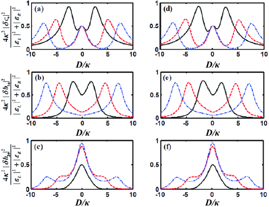
Fig. 4: Comparison of identical and non-identical NRs in the variation of photon and phonon numbers with respect to the probe detuning $D/\kappa$. The panels: (a) and (d) for the normalized probe photon number $\frac{4\kappa^{2}}{|\varepsilon_{L}|^{2}+|\varepsilon_{R}|^{2}}|\delta{c}_{+}|^{2}$; (b) and (e) for the normalized mechanical excitation $\frac{4\kappa^{2}}{|\varepsilon_{L}|^{2}+|\varepsilon_{R}|^{2}}|\delta{b}_{1+}|^{2}$; (c) and (d) for $\frac{4\kappa^{2}}{|\varepsilon_{L}|^{2}+|\varepsilon_{R}|^{2}}|\delta{b}_{2+}|^{2}$. (a), (b) and (c) plot identical NRs with $D=\omega_{p}-\omega_{c}-\omega_{m}$, while (d), (e) and (f) present non-identical NRs ($\omega_{2}=1.2\omega_{1}$) with $D=\omega_{p}-\omega_{c}-\omega_{1}$. The black solid, red dashed, and blue dashed-dotted curves are for pumping rates $|G|=2\kappa$, $4\kappa$, $6\kappa$, respectively.

From Figs. 4 and Table 1, we find in the case of identical NRs that, when the inverse OMIT takes place, the sum of the mechanical excitations [$\frac{4\kappa^{2}}{|\varepsilon_{L}|^{2}+|\varepsilon_{R}|^{2}}(|\delta b_{1+}|^{2}+|\delta b_{2+}|^{2})\equiv 1$] is always double of the intracavity probe photon number [$\frac{4\kappa^{2}}{|\varepsilon_{L}|^{2}+|\varepsilon_{R}|^{2}}|\delta c_{+}|^{2}=0.5$]. This implies that the energy distribution in the two NRs and the cavity field always remains with the ratio $2:1$. Besides, with increase of $|G|$ and $\lambda$, the phonon distribution in the two NRs varies in different ways conditional on the channels. For two different NRs, there is a small deviation with respect to the identical case, and only the middle channel satisfies the condition for the inverse OMIT. These characteristics of our multi-channel inverse OMIT are very different from in previous schemes [44, 45].

4.3 Measurement of the relative phase in a unilateral inverse OMIT

Since the inverse OMIT is resulted from the perfect destructive interference between two probe lights along opposite directions [44], any imperfection, such as a phase difference between the two probe lights, would lead to deviation from the perfect destructive interference. As such, it would be interesting to explore the possibility of detecting the difference between the two probe lights in an imperfect inverse OMIT.

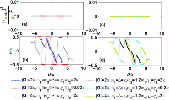
Fig. 5: (a) and (c) The strength of the output light from the left-hand side of the optomechanical cavity with different probe light detunings, which remains unchanged for different parameter values; (b) and (d) The phase $\theta$ of the unilateral inverse OMIT for different probe light detunings. The left-hand side panels are for identical NRs ($\omega_{2}=\omega_{1}$) with $D=\omega_{p}-\omega_{c}-\omega_{m}$, while the right-hand side panels for non-identical NRs ($\omega_{2}=1.2\omega_{1}$) with $D=\omega_{p}-\omega_{c}-\omega_{1}$.

After a relative phase $\theta$ is introduced in the probe light input from the right-hand side of the cavity, the inverse OMIT observed in the left-hand side takes the form

$$\begin{array}[]{ccc}\varepsilon_{outL+}=\frac{2\kappa(\varepsilon_{L}+\varepsilon_{R}e^{i\theta})}{2\kappa+i(\Delta-\delta)+\frac{|G|^{2}}{\frac{{\gamma_{1}}}{2}-i(\delta-\omega_{1})+\frac{{\lambda^{2}}}{{\frac{{\gamma_{2}}}{2}}-i(\delta-{\omega_{2}})}}}-\varepsilon_{L}&=&0.\end{array}$$ (17)

In contrast to the same output lights ($\varepsilon_{outL+}=\varepsilon_{outR+}$) from both sides of the cavity, the inverse OMIT involving a relative phase outputs the lights with $\varepsilon_{outL+}\neq\varepsilon_{outR+}$, implying that the inverse OMIT, if occurring, is observed only on one side of the cavity (i.e., an unilateral OMIT). In such an unilateral inverse OMIT, the relative phase $\theta$ is found to be monotonously varying with the detuning $D$ within some parameter regimes, which can be employed for evaluating $\theta$ (see Fig.5).

Provided that the strengths of the two probe lights are the same ($\varepsilon_{L}=\varepsilon_{R}$), the above equation is reduced to

$$\begin{array}[]{ccc}\frac{|G|^{2}}{\frac{{\gamma_{1}}}{2}-i(\delta-\omega_{1})+\frac{{\lambda^{2}}}{{\frac{{\gamma_{2}}}{2}}-i(\delta-{\omega_{2}})}}-i(\delta-\Delta)&=&2\kappa e^{i\theta}.\end{array}$$ (18)

Straightforward deduction using the relations among $D$, $\delta$ and $\Delta$ yields that, the relative phase $\theta$ is a function of the detuning $D$, as plotted in Fig. 5(b) and Fig. 5(d), and not all the frequencies of the probe lights can generate the unilateral inverse OMIT effect.

For a precision measurement of $\theta$, choosing qualified regimes of the parameters, e.g., $D/\kappa\in[-1.5,1.5]$, is necessary to obtain a monotonous change of $\theta$ with $D$. Besides, for the measurement to be more precise, we expect a large change of $D$ for tiny variation of $\theta$, implying a small slope of $\Delta\theta/\Delta D$. As such, smaller radiation coupling is optimal [see the curves in Fig. 5(b) with $|G|=2\kappa,4\kappa$ and note the lower limit $|G|\geq\sqrt{8/3}\kappa$]. In comparison with the identical NRs [in Fig. 5(b)], the curves for the non-identical NRs [in Fig. 5(d)] own smaller slopes, implying a better measurement. For example, in the case of $D/\kappa\in[-0.01,0.01]$, the measurement sensitivity $\Delta D/\Delta\theta$ is 6.3 MHz/$\mathrm{rad}$ for the blue curve in Fig. 5(b), and 7.7 MHz/$\mathrm{rad}$ for the black curve in Fig. 5(d). So elaborately choosing different NRs can be favorable for enhancing the measurement precision of $\theta$. By numerical simulation of Eq. (18), we find the largest measurement sensitivity $\Delta D/\Delta\theta=$8.3 MHz/$\mathrm{rad}$ at $\omega_{2}/\omega_{1}=1.346$, since the unilateral inverse OMIT would disappear once $\omega_{2}/\omega_{1}>1.34$.

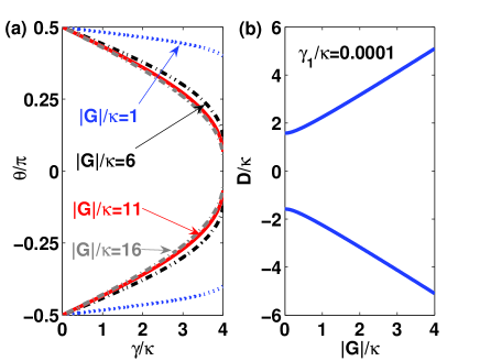
Fig. 6: (a) The decay of the NR versus the relative phase between two probe lights for different effective radiation couplings; (b) The detuning of the probe field from the cavity resonance frequency verses the effective radiation coupling, where $\Delta=\omega_{1}$ and $D=\delta-\omega_{1}=\delta-\Delta$.

Moreover, this unilateral inverse OMIT can also be applied to typical optomechanical cavity with only one NR. For example, when the Coulomb coupling is decoupled, Eq. (18) can be reduced to

$$\begin{array}[]{ccc}\frac{|G|^{2}}{\frac{{\gamma_{1}}}{2}-iD}-iD&=&2\kappa e^{i\theta},\end{array}$$ (19)

for $\Delta=\omega_{1}$ and $D=\delta-\omega_{1}=\delta-\Delta$. Then we obtain the corresponding detunings for the unilateral inverse OMIT as

$$D_{\pm}=\pm\sqrt{\frac{1}{8}(8|G|^{2}+(16\kappa^{2}-{\gamma_{1}^{2})}+\sqrt{16|G|^{2}(16\kappa^{2}-{\gamma_{1}^{2}})+(16\kappa^{2}+{\gamma_{1}^{2}})}}.$$ (20)

With the assistance of Eq. (19), the decay of the NR versus the relative phase between two probe lights is calculated with respect to different effective radiation couplings, as plotted in Fig. 6(a). It implies that the unilateral inverse OMIT can be observed for any decay rate of the NR, which is a great improvement on the inverse OMIT compared to that in [44], where the inverse OMIT can only be achieved when $4\kappa={\gamma_{1}}$. Besides, we numerically treat Eq.(20) in Fig. 6(b), showing that the detuned frequency for the unilateral inverse OMIT is almost linear to the effective radiation coupling with a ratio $\Delta|G|/\Delta D=1.016$, and thus the effective radiation coupling can be identified by the detuned frequency in this way.

5 The experimental feasibility

We exemplify the unilateral inverse OMIT for a brief discussion about the experimental feasibility of our scheme. In terms of the experimental parameters in [59], we set following parameter values available using current techniques: The frequencies of the NRs $\omega_{1}\simeq\omega_{2}=2\pi\times 947$ kHz, $m_{1}\simeq m_{2}=145$ ng, the cavity wavelength $\lambda_{c}\equiv 2\pi c/\omega_{c}=1064$ nm, the cavity length $L=25$ mm, and the cavity decay rate $\kappa=2\pi\times 215$ kHz. Then the effective radiation coupling is $|G|=g_{0}|c_{s}|=\hbar\omega_{c}/L|c_{s}|\geq 2\pi\times 351$ kHz corresponding to the Coulomb coupling strength $\lambda\geq 2\pi\times 124$ kHz [33, 46, 48, 60, 61] and the strength of the driven light field $\varepsilon_{c}=\sqrt{2\wp_{c}\kappa/\hbar\omega_{c}}$ with a input power $\wp_{c}\geq 0.037$ mW.

The prerequisite of observing an inverse OMIT is a near red-sideband resonance ($\Delta\simeq\omega_{1}$). Considering the requirement for sideband resolution, we may rewrite the condition of the near red-sideband resonance more specifically as $0\leq|\Delta-\omega_{1}|\ll\omega_{1}$. In the case of an exactly red-sideband resonance, we have a symmetrical inverse OMIT. When there is a tiny deviation from the exactly red-sideband resonance, but satisfying $0<|\Delta-\omega_{1}|\ll\omega_{1}$, we have an asymmetrical profile and in this case the inverse OMIT still occurs. The possibility lies in following points: i) The OMIT originates from the quantum interference generally with an asymmetrical profile, and the symmetrical profile is a special case; ii) The phase shift in the destructive interference is generated by the ratio between the dispersion and the absorption caused by the quantum interference. As such, our scheme can work within the regime: $0<|\Delta-\omega_{1}|\ll\omega_{1}$.

6 Conclusion

In summary, we have investigated a tunable multi-channel inverse OMIT in the optomechanical system with the assistance of the Coulomb interaction between two charged NRs. Our results have shown both analytically and numerically three channels for perfectly absorbing the input probe fields at different frequencies in such a system, which makes it possible to select a desired frequency of inverse OMIT by adjusting effective radiation coupling rate and the corresponding Coulomb coupling strength. Some applications have been discussed based on the considered model. We believe that our study would be useful for further understanding the inverse OMIT and exploring the applications of the inverse OMIT.

Based on the schematic in Fig. 1, our scheme can be extended to other systems such as a waveguide optomechanics [35] and the Coulomb coupling between two NRs by a bias voltage gate [51]. We have noted the opto-mechanical experiments reported recently with NRs coupled by tunable optical coupling [49] and fixed elastic coupling [50]. Replacing the Coulomb coupling by those couplings, our model can immediately apply to those opto-mechanical systems in [49, 50]. In addition, we are also aware of a recent work for a multi-channel inverse OMIT by confining many NRs in a single cavity [43]. The idea is very interesting, but much more difficult to achieve experimentally than our scheme.