On the Role of Conductance, Geography and Topology in Predicting Hashtag Virality

Abstract

We focus on three aspects of the early spread of a hashtag in order to predict whether it will go viral: the network properties of the subset of users tweeting the hashtag, its geographical properties, and, most importantly, its conductance-related properties. One of our significant contributions is to discover the critical role played by the conductance based features for the successful prediction of virality. More specifically, we show that the first derivative of the conductance gives an early indication of whether the hashtag is going to go viral or not. We present a detailed experimental evaluation of the effect of our various categories of features on the virality prediction task. When compared to the baselines and the state of the art techniques proposed in the literature our feature set is able to achieve significantly better accuracy on a large dataset of 7.7 million users and all their tweets over a period of month, as well as on existing datasets.

1 Introduction

The ability to predict the emergence of virality of a hashtag has far-reaching consequences in a number of domains. In the commercial domain knowledge of potentially viral memes may present a variety of business opportunities but the most important application of a robust prediction system would be to provide the authorities with the capability of spotting the emergence of harmful rumors and the organization of destructive mass action. For example, the role of Twitter and Blackberry messenger in organizing looting and spreading rumors was widely observed during the London riots of 2011 [5]. In 2008 live accounts of the Mumbai terror attacks went viral on Twitter spreading panic and providing the attackers with a source of information on police movements [28]. In both cases early detection of the spread of a particular kind of meme could have helped arrest it and prevent disastrous consequences. The nature of such settings is that they require a prediction system to sift out important (potentially viral) content from the vast volume of content in the network. The usual metrics, precision and recall, take on special significance here. High recall ensures that we do not miss a potentially harmful meme, while high precision ensures that expensive resources are not expended on investigating false leads. In this paper we present prediction algorithms for Twitter, although we feel that techniques using similar features can be used on other social networks (like those derived from cellular messaging or calling data) as well and so will have wide applicability.

Studying the factors that lead to virality in online systems has been an important theme in the literature over the last few years, pioneered by Leskovec, Backström and Kleinberg’s study of the evolution of memes in blogs [23]. The phenomenon of virality wherein a particular meme–a theme or topic or piece of content–spreads widely through the network has, in particular, attracted a lot of attention. What has been largely missing is prediction that focuses on the efficacy of structural properties of meme diffusion. The only efforts of this nature are the two attempts by Weng et. al. [36, 35] and their work, on a user network of about 0.6 million users is not conducted on a satisfactorily large scale. We undertake a classification task on a large dataset that we compiled containing 7.7 million Twitter users and all their tweets over a 35 day period. For every hashtag in our set that appears in a certain number of tweets (we call this number the prediction threshold and set it to 1500 in this paper) we try to predict, at the point when it reaches this number, if it will reach a number of tweets about one order of magnitude larger. This latter number, we call it the virality threshold, is set to 10,000. In what follows we will refer to this task as virality prediction. The features that we use for this classification task deliberately ignore the content of the tweeted hashtags, focusing instead on three aspects: network topology, geography, and the isoperimetric properties of meme growth as expressed through the conductance of the set of users tweeting on a hashtag. This should not be seen as a claim that these characteristics are more important than semantic aspects of the topics under study. We omit using semantic features to maintain a focus on the predictive power of structural properties of hashtags. It is not our intention to present a “best possible” prediction algorithm; such an algorithm would undoubtedly include semantic features along with our structural and geographic features. Our intention is primarily to demonstrate that there is significant information contained in our new features based on conductance, geography and network characteristics of early adopters, and that this information can be effectively used in the important task of predicting virality.

We view the evolution of the hashtag’s spread across the network as a graph process and derive a number of network-based features. The geographical spread of hashtags is also used for virality prediction for the first time, enabled by a methodology that is successfully able to tag 90% of active users with their time zones. We define features based on the isoperimetric quantity conductance that is known to have a strong relationship to mixing times in random walks [14], and find that these features greatly help improve our predictions. We use the criteria of information gain to identify the top features from each category providing us greater insight into the effectiveness of various features for characterizing virality.

We perform an extensive experimental evaluation of our proposed set of features for the task of predicting virality. Our experimental results clearly demonstrate the effectiveness of our features for this task as well as their supremacy over existing approaches proposed in the literature. We also present some preliminary experimental analyses of virality prediction in individual geographies which corroborate our findings in the larger dataset.

Organization

We survey the literature in Section 2, following that with a description of our dataset and how it was compiled in Section 3. Our task definition can be found in Section 4, followed by a detailed discussion of our features in Section 5 and the results of our algorithms on two datasets in Section 6. Finally we conclude with a discussion of the significance of conductance and some future directions in Section 7.

2 Related Work

The problem of predicting which memes will grow in popularity has attracted some amount of attention recently. To save space we ignore the research on detecting popularity after it has been established and focus on the research on identifying memes that will go viral before they have already spread far and wide. Several aspects of this problem have been studied. Wu and Huberman, in an early paper, highlighted the importance of novelty: new memes override older ones [37]. In a similar vein, Weng et. al. [34] argued that finite user attention coupled with the structure of the network can help identify the ultimate popularity of a meme. Emotional, textual and visual features have been studied as drivers of virality [4, 13, 12, 33, 15]. In the context of viral marketing, Aral and Walker showed that personalization of promotional messages helps make particular products more “contagious” [2].

While all these aspects are undoubtedly important, our work falls into a different category of research which views the proliferation of memes as a kind of contagion process on a network and relies on spatial and temporal properties of the early evolution of this process to identify potentially viral memes. Leskovec et. al.’s work on memes falls into this category, positing a temporal growth model for viral memes [23]. With the growth of microblogging it was natural that such phenomena be investigated on Twitter and Kwak et. al. [21] performed the first analysis of information spreading on Twitter at scale. Subsequently, several groups of researchers have investigated the structural properties of rapidly spreading themes by looking at the spread as a cascade or a tree (e.g. Ghosh and Lerman [10]). Others tried to find the extent of external (or exogenous) influence on information diffusion (e.g. Myers et. al. [27]). Szabo and Huberman tried to predict the long-term popularity of a meme based on its nascent time series information [32]. Kitsak et. al. argued that the most efficient spreaders are those that exist within the core of the network and the distance between such spreaders often governs the maximum spread of topics [19]. The factors that govern a tweets ability to draw retweets, a possible precursor to virality, has been studied by Suh et. al. [31]. On the modeling front, Romero et. al. focused on the local dynamics of hashtag diffusion [30]. Lermann et. al. [22] propose an approach to predict popularity of news items in Digg using stochastic models of user behavior. Rajyalakshmi et. al. defined a stochastic model for local dynamics with implicit competition that was found to generate the global dynamics of a Twitter-like network [29]. Finally we mention the work that is the major take off point for our current paper: Ardon et. al. conducted a study of information diffusion on a large data set and established that conductance and geographical spread could significantly discriminate between topics that went viral and those that did not [3]. Drawing on ideas from this work we create suite of features and show that they can be used effectively to predict virality.

Efforts to use machine learning techniques to predict virality have recently begun to appear in the literature. Jenders et. al. use features very different from ours, relying mainly on sentiment-related features, to predict which tweets will go viral via the process of retweeting on a small data set of 15,000 users [17]. Zaman et. al. use a Bayesian approach to predict which tweets will generate large retweet trees on a small set of 52 tweets [38]. Ma et. al. combine a set of textual features with some network-based features to predict the number of users tweeting a hashtag in subsequent time intervals, a task somewhat different from ours since we focus on predicting an eventual ascent to a threshold-based virality [25]. In a major recent work, Cheng et. al. tried to predict which photo resharing cascades will grow past the median cascade size using a variety of features that included demographic, structural and temporal information [6]. The primary difference between that work and ours is that we do not work with a cascade model, but look at the spread of hashtags as a diffusion, i.e., the use of hashtag by a particular user need not be explicitly attributable to the prior use of that hashtag by another user in the neighborhood. This makes our work incomparable with that of Cheng et. al. [6] and gives it a different flavour. Closer to our approach in conception if the work of Weng et. al. who showed in a sequence of two papers that inter-community spread in the early life of a Twitter meme can be used to predict which meme will go viral and which will not [36, 35]. The main work against which our results should be compared is [35] where a straightforward attempt to predict virality is made, as opposed to [36] where a related but slightly different multi-label classification task is defined. Our current work overcomes some of the severe shortcomings of [36, 35]. Firstly, we perform prediction on a user set of size 7.7 million and view their interconnections as a directed graph. In [36, 35] the user set has size only 0.6 million and consists of edges only between those users who follow each other, i.e. only bidirectional edges. Secondly, the small size of their network allows Weng et. al. to run community detection algorithms which are prohibitively expensive to run. We show that on our much larger data set, to the best of our knowledge the largest on which virality prediction tasks have been run so far, by leaving out community-based features and using computationally tractable features based on geography and conductance we are able to give better quality predictions than those in [35]. We also show that our feature set performs better than the community-based features of Weng et. al. [35] on their own data set, even though we do not have the geography information for their users.

3 Dataset and Methodology

3.1 Dataset description

Our dataset is a complete snapshot of all tweets posted by 7.7 million users of Twitter between 27th March 2014 and 29th April 2014. We also have the follower-following information of all these users and have built the data set (as explained below) to ensure that these users form a strongly connected subnetwork of Twitter, i.e., for each pair of users $u,v$ there is a directed path $u$ to $v$ and a directed path from $v$ to $u$. Rather than filtering out tweets based on topical memes, we crawled all the tweets posted by our user set in the time window with a view to capture all the phenomena, viral and non-viral, present in the network at the time.

Users	7,695,882
Average no. of followers	450
Users who tweet at least once	3,008,496
Filtered hashtags	8,793,155
Tweets for filtered hashtags	220,012,557
Hashtags with $\geq$ 10,000 tweets	177

Table 1: Dataset statistics

Table 1 contains some basic statistics of our data set. The follower distribution curve of our data (see Figure 1) follows the now familiar power law with a drooping tail that has been widely reported in the literature.

From the tweets of our user set we extracted all the hashtags used, filtering some persistent generic hashtags out (as explained in Sec 3.3.)

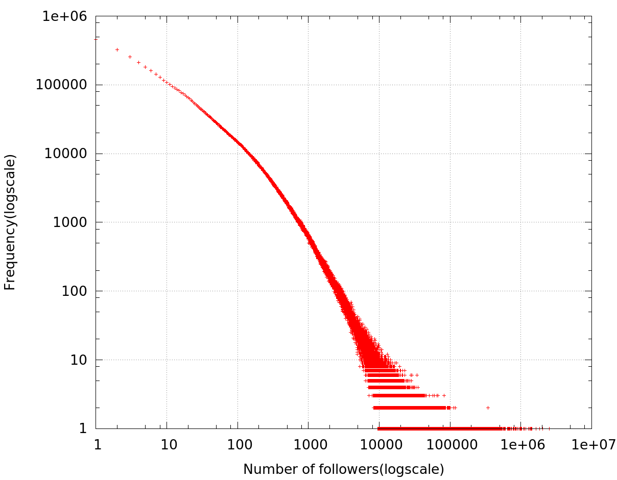
Figure 1: Plot of the distribution of the Number of followers

Additionally we geotagged all the users who have tweeted at least once with their location information to an accuracy of 98%, not down to the city level but down to the time zone level using the time zones that Twitter requires users to fill through a dropdown menu at the time of account creation. There were 141 time zones found in our data set. We note that Twitter provides annotated time zones that are more numerous than the 40 different time offsets from UTC that are generally used for timekeeping. For example, although all of India follows a single time (Indian Standard Time: UTC +5:30), Twitter gives Indian users four choices–Chennai, New Delhi, Kolkata, Mumbai–corresponding to four major metropolitan centres, all of which are marked as GMT +05:30 in the dropdown.

3.2 Retrieving the data from Twitter

A seed set of approximately 108K users was shared with us by Pranay Agarwal who devised a methodology for differentiating users whose tweets were informative from those users who used Twitter as a forum for chatting [1]. The seed set comprised users whose tweets were generally informative in nature, ensuring that our user set is focussed on a subset of users who transact emergent memes. We extracted the follower and following information of this seed set and computed the strongly connected component that turned out to be of size 64K. We then queried Twitter for all the users who were either following or followed by these 64K users. This gave us an initial set of 9,188,701 users.

We then used the “GET followers” method of the Twitter API to extract the follower and following information of these 9.1 million users. We were successful in extracting this information for 8,379,871 users. The remaining users had their accounts suspended or their follower and following information was protected. We computed the strongly connected component of this reduced set. Its size was found to be 8,047,811.

Using the “GET user_timeline” method from Twitter’s REST API (v 1.1) we collected tweets from these 8.04 million users’ timelines. The GET user method provides the 3200 most recent tweets of each user and so in order to build a dataset of at least a month’s duration we repeated the crawl after 10 days. The first crawl began on 18th April and ended on 20th April. The second crawl began on 30th April and ended on 2nd May. The two crawled sets were then combined to finally obtain all the tweets posted from 27th March to 29th April 2014, without duplication or omission. This process of combination involved discarding 26,624 of the users whose high frequency of tweeting made it impossible to guarantee that we had captured all their tweets in this 35 day time span. After removing these 26,624 users we recomputed the strongly connected component of the remaining network and found it to have size 7,695,882. These 7,695,882 users with their interconnections formed our final user network.

3.3 Filtering the hashtags

On examination we found that the most frequently occurring hashtags in the tweet dataset created were generic hashtags that persist on twitter with a very high frequency of occurrence e.g. #rt, #tlot, #win, #giveaway and #jobs. In order to filter out these hashtags and obtain a set of hashtags that are fresh in our time span and thereby refer to emergent phenomena we filtered out all the hashtags that had more than 5 tweets in the first 12 hours of our time duration.

Hashtag	Tweets
bundyranch	395,179
nashto2mil	152,657
votekatniss	140,031
votetris	135,206
epnvsinternet	104,575

Table 2: Top 5 hashtags in our dataset

Table 2 shows the 5 most popular hashtags in our dataset after filtering along with the number of tweets for each of them. The first one, “bundyranch”, refers to a major US news story of the time. The second one commemorates a Twitter celebrity Nash Grier’s follower count reaching 2 Million. The third and fourth are related to voting prior to the MTV Movie awards that were held on 13th April 2014, and the fifth one “epnvsinternet” is part of a mass action by civil organizations in Mexico to oppose a proposed legislation. These five demonstrate anecdotally that our filtering process does generally capture emergent topics on Twitter and also that endogenous topics generated from within Twitter like “nashto2mil” and exogenous topics like “bundyranch” and “votekatniss” are both present in our dataset.

3.4 Geolocating the users

Twitter users have the option of specifying their time zone, their country and their location. The first two of these are populated from a dropdown menu and the third is entered as a string and hence is often hard to map to an actual geographical location. These three fields are part of the user’s profile and are embedded in the JSON object containing the user’s tweet, which is where we extracted them from. This JSON object also contains geo-coordinates from tweets posted from GPS-enabled devices whose users have allowed this information to be shared but we found that to be a rare occurrence and not of much use.

Time Zone	Users
Eastern Time (US & Canada)	967,849
Central Time (US & Canada)	636,541
Pacific Time (US & Canada)	549,611
London	395,738
Quito	212,584

Table 3: Top 5 time zones in our dataset

On examination we found that timezone was a widely present attribute, missing only from 630,696, i.e., 11.9% of the 5.3 million users who had posted at least one tweet in our initial set of 9.1 million users. About a third of these users, 217,443, had tweeted from GPS-enabled devices and so we were able to map them to time zones using the Google Time Zone API. For the remaining users we extracted their location string and tried to map it to a time zone by using common substring heuristics to match their location strings with popular cities and with location strings of users that have their time zones set. This helped us locate another 118,488 users. Finally, we were left with 294,765 users. To these users we assigned the time zone in which the maximum number of their neighbors were located. Testing this heuristic on users whose location was known we obtained a 48% success rate. So, in summary, we were able to correctly geolocate all but 294,765 users out of 5.3 million, i.e., 94.4% of our users. The remaining 5.6% were tagged with a heuristic that we expect to perform correctly about half the time. Even if we consider only the subset of 3 million users who tweet once in our 35 day period and assume that the 294,765 users whose location we guess all lie in this subset, we see that 90% of our users are correctly tagged and the remaining 10% are tagged by a heuristic that has 48% accuracy. We note that there have been several research efforts made to geolocate users but they have been either at the country level e.g. [20] or at a fine-grained level of tens of kilometers e.g. [26]. We adopt a simpler strategy here to achieve geo-location at the intermediate granularity of Twitter time zones since geo-location is not the primary focus of our paper. As reported we find that the accuracy we achieve using our simple, and computationally efficient, methods is significant and good enough for our purpose. Table 3 lists the top five time zones by population in our user set. We see that along with what we traditionally understand by time zones like “Eastern Time (US & Canada)”, we also have individual cities like “London” and “Quito.”

4 Prediction Task

The goal of our study is to examine how successfully we can discriminate viral topics from non-viral ones based on their early spreading pattern. In this section we make this goal concrete. We undertake here a classification task whose objective is to predict at a particular, early, point in the spread of a hashtag whether that specific hashtag will, in the future, enter the class that we define as viral.

Defining virality

Various definitions of virality have been used in the literature. One of them is based on calling a topic viral if it is among the top $k$% (for some small value of $k$) of all the topics ranked by their total number of tweets. This definition has been used by Weng et al. [35] for values of $k$ starting at 10. A drawback of this definition is that, because of its relative nature, it is non-monotonic. In other words, a topic may become viral at a given point of time, but then be declared non-viral at a later point in its life when some other topics have surpassed it in terms of number of tweets and it is no longer in the top $k\%$. While it is definitely true that a viral topic ceases to be viral after some time, to make this percentile-based definition stick we would also have to provide some kind of time window within which the topic must remain in the top $k$%. In order to avoid such complications we decided to use an alternate definition based on an absolute threshold, i.e., we say a topic has become viral if its total number of tweets cross a certain given threshold $M$. We call this the virality threshold. We used $M=10,000$ in our experiments. This number has no intrinsic significance. It is based on the sizes of the spreads of various hashtags in our data set. Note that while we saw in Table 2 that the 5 largest spreading tags had more than 100,000 tweets, choosing a virality threshold of 10,000 gives us only 6.29% of hashtags. This top 6.29th percentile that we consider viral is significantly smaller than the 10th percentile that is taken as viral by Weng et al. [35].

Prediction threshold

Since we are interested in predicting the future spread based on early history, we decided to extract features from the first $n=1500$ tweets. We call this value $n$ the prediction threshold. In other words, for each hashtag, we examined its spread in the network upto the point the $1500$th tweet containing that hashtag was posted and extracted various features based on this early spread. All the topics which did not cross the $n=1500$ tweet mark were ignored for the purpose of our study. The total number of hashtags that we were left with was 2810, of which 177 crossed the virality threshold.

Choosing a very small value of $n$ may not give us sufficient information about the topic spread but a very large value of $n$ will make the prediction meaningless as the peak would already be reached (or be very close). So, it is important to choose $n$ in an appropriate manner. Further note that the choice of appropriate $n$ would also depend on the size of the dataset. For a large dataset $n$ would be higher compared to a smaller dataset simply because of the sheer volume of tweets generated in the network. To put in context our choice of $n=1500$, another similar recent study by Weng et al. [35] has used $n=50$ tweets as their threshold. The size of their dataset (in terms of the number of users) is about 5% of the size of the dataset that we use (595K nodes vs 7.7 million nodes). In order to show that these two prediction threshold values, Weng et. al’s 50 and our 1500 are similar we plotted the time taken to reach $n=1500$ tweets for a particular hashtag in our dataset and the time taken to reach $n=50$ tweets in the dataset of Weng et. al. [35]. In Figure 2 we have time on the $x$-axis and the fraction of hashtags that take at most a given time to reach the prediction threshold for our dataset (TwitDat) theirs (WengDat). The overlapping nature of the two curves clearly demonstrates the similarity in the behavior of the topics at the two prediction thresholds for the two datasets, respectively. The median time taken to reach the prediction threshold is $12.38$ days for our data set and $13.03$ days for Weng et al’s. We interpret these results to mean that the amount of information available at our prediction threshold for our dataset closely aligns with the amount of information available in the other prediction threshold for the other major study, and hence our results can be compared with theirs.

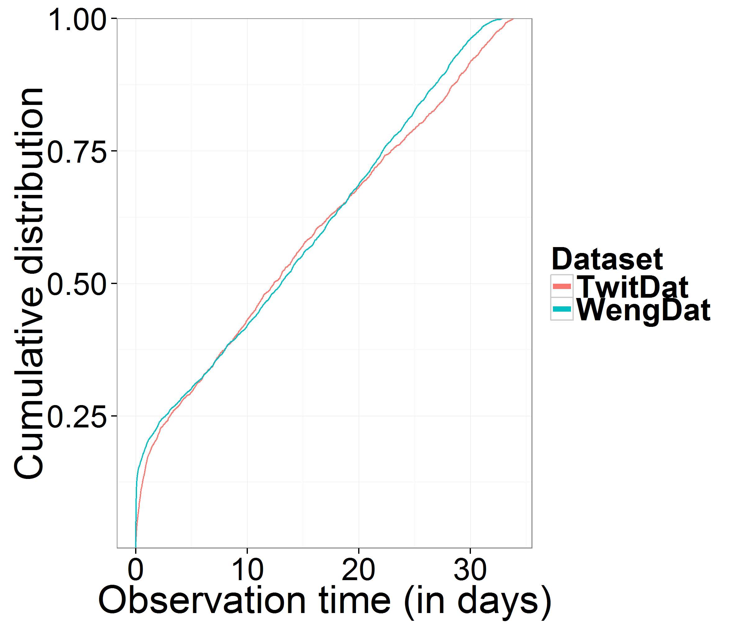
Figure 2: Time taken to reach the prediction threshold.

5 Our features

The main contribution of this paper is the definition of a set of novel features that are critical to the task of predicting virality. We propose a number of new features and argue that one of the most important aspects of early hashtag growth is the rate of change of the conductance of the subset of nodes that are tweeting the hashtag. Our prediction algorithm is also the first to incorporate a set of geography based features. Apart from our conductance and geography based features we also use a set of temporal features (we call these “evolution based features”) and a set of features that capture the network characteristics of the early tweeters of a hashtag. In total we have experimented with $29$ different features. The features are listed in Table 4.

We will refer to the users who tweet on a hashtag up to the prediction threshold as adopters of that hashtag. Of these a special category are what we call self-initiated adopters who tweet on a hashtag before any of the users that they follow do so. In some places we will use the term “topic” interchangeably with “hashtag”. The term “geography” will be used to denote Twitter time zones as described in Section 3 e.g., if we say “the average number of users in a geography is X” we mean that the average number of users in a Twitter time zone is X. Further, we will use the term weakly connected component in the way it has come to be understood i.e. given a directed graph if we treat each directed edge as undirected and compute the connected components of the transformed graph, then each of these connected components is known as a weakly connected component of the original directed graph.

Name	Description
Evolution based features
NumOfAdopters	Number of adopters who tweeted on the hashtag
NumOfRT	Number of retweets (RT) on tweets within the prediction threshold
NumOfMention	Number of user mentions (@) in tweets within the prediction threshold
TimeTakenToPredThr	Growth rate of the hashtag measured in terms of time taken to reach prediction threshold
Network based features
HeavyUsers	Number of adopters with at least $3000$ followers
NumFolAdopters	Total number of followers of adopters
NumOfEdges	Number of edges in the network spread, i.e., the subgraph induced by the set of adopters
Density	Subgraph density
SelfInitAdopters	Number of Self-initiated adopters
SelfInitAdoptersFollowers	Total follower count of Self-initiated adopters
RatioOfSingletons	Ratio of Self-initiated adopters to number of adopters
RatioOfConnectedComponents	Ratio of number of weakly connected components to number of adopters
LargestSize	Size of the largest weakly connected component
RatioSecondToFirst	Ratio of sizes of the second largest to the largest weakly connected components
Geography based features
InfectedGeo	Number of infected geographies
RatioSelfInitComm	Fraction of Self-initiated geographies
RatioCrossGeoEdges	Fraction of edges across geographies in the induced subgraph of adopters
AdoptEntropy	Adoption Entropy measures the distribution of adopters across geographies and is defined as $-\sum\limits_{i}a_{i}\log a_{i}$, where $a_{i}$ is the fraction of adopters in each geography $i$
TweetingEntropy	Tweeting Entropy measures the distribution of tweets across geographies and is defined as $-\sum\limits_{i}t_{i}\log t_{i}$, where $t_{i}$ is the fraction of tweets in each geography $i$
IntraGeoRT	Fraction of retweets occurring between users from the same geography
IntraGeoMention	Fraction of user mentions occurring between users from the same geography
Conductance based features
CummConductance	Conductance of the subgraph induced by the set of adopters
Conduct’_k, $k=~{}\{20,50,100,250\}$	First derivative of conductance for different values of smoothing parameter $k$
Conduct”	Second derivative of conductance
Conduct’_stdev, Conduct”_stdev	Standard deviation of first and second derivative of conductance

Table 4: Feature descriptions. All features have been captured with respect to tweets within the prediction threshold

5.1 Feature Categories

We divided our features in the following four categories: 1) Evolution based features capture very basic analytics of the hashtag’s evolution such as number of adopters, number of retweets, number of user mentions and growth rate of the topic. Since these are very simple features we will be using them to generate baselines. 2) Network based features include various network characteristics of the adopters of the topic in terms of their followers, density, self-initiated adopters and weakly connected component based features. 3) Geography based features capture the geographical properties of the spread such as number of infected geographies, intra and inter geography features, number of self-initiated adopters in each geography etc. 4) Conductance based features, though based on network properties, have been put in a separate category due to their prime importance for the task of characterizing virality. These include conductance as well as its first and second derivative. Next we discuss the features in each of the above categories.

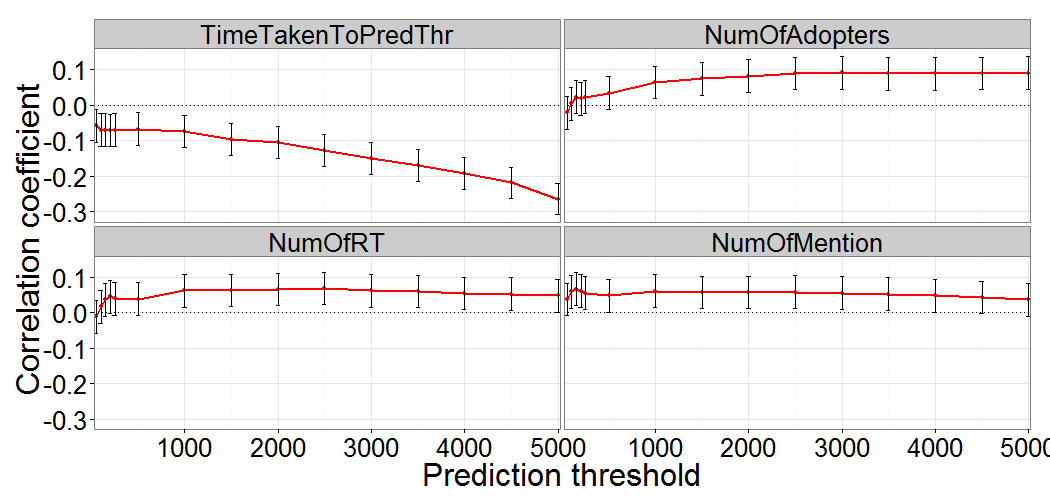
(a) Evolution based features (E)

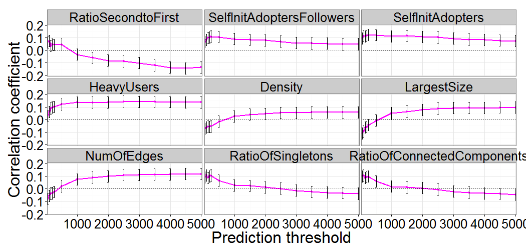
(b) Network based features (N)

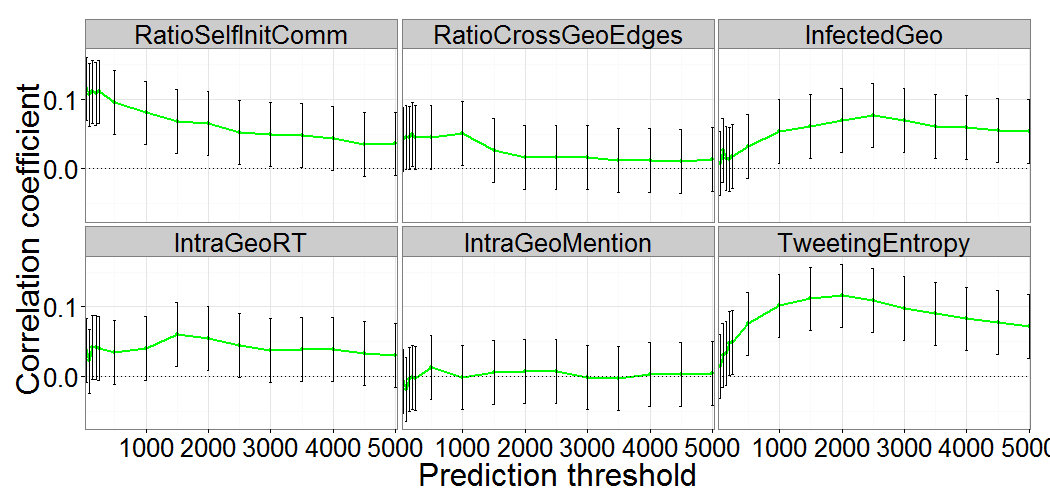
(c) Geography based features (G)

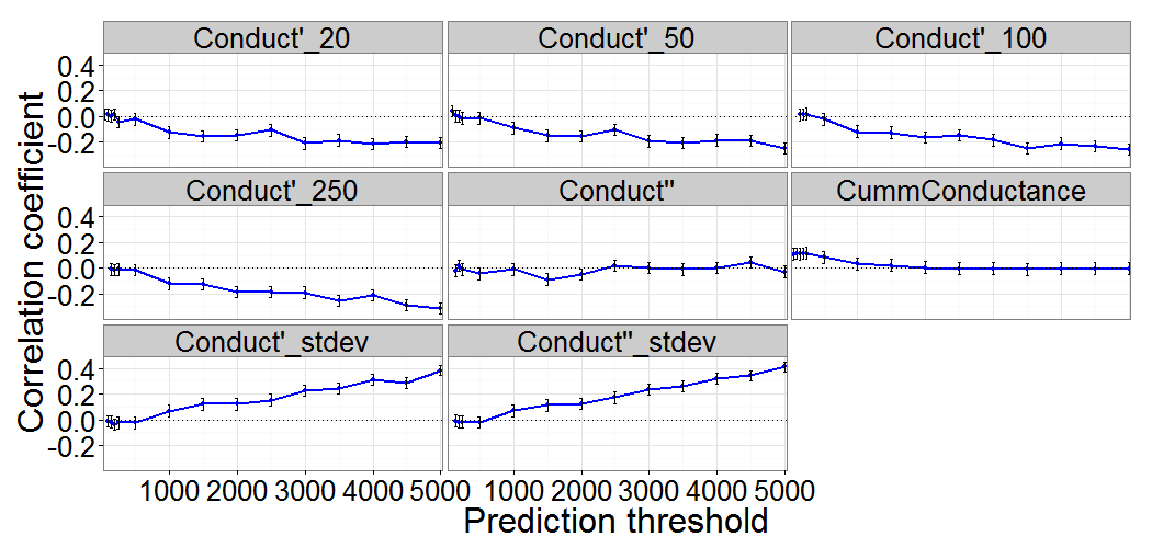
(d) Conductance based features (C)

Figure 3: Change in correlation coefficient with increase in number of tweets. Bars indicate the $95\%$ confidence interval

5.1.1 Evolution-based features

These features include basic characteristics about the topic evolution and include the following $4$ features: 1) Number of Adopters 2) Number of Retweets 3) Number of User Mentions 4) Growth Rate defined as the time taken to reach the prediction threshold. We group these in two sets, denoting the first and the fourth features as the set E1, and the second and third as E2. We note that the first two features have been used before by Weng et. al. [36, 35]. Growth Rate was used, along with a number of variations thereof, by Cheng et. al. [6]. Zaman et. al. [38] used the number of retweets and other aspects of retweeting as features for their prediction task while Jenders et. al. [17] used number of user mentions as a feature. For us, as mentioned earlier, this set of features will be used to create non-trivial baselines. The first baseline will use only the features E1 while the second baseline will use all four features. The details of how these baselines will be used are discussed in Section 6.

We plotted the change in Spearman’s rank correlation coefficient, measured between feature values and total hashtag growth, with increasing number of tweets for all hashtags that had at least 5000 tweets (see Figure 3(a)). For the feature set E we find the number of adopters and number of RTs are positively correlated with hashtag growth but the correlation levels out, while the time to prediction threshold is highly negatively correlated and continues to grow in this direction. This latter observation is similar to that of Cheng et. al. [6] who observed that successful cascades get many views in a short amount of time.

5.1.2 Network-based features

We used the following $10$ network based features (divided into 3 sub-categories) for our study. The first subset includes features based on adopters and their connections: 1) Number of Adopters with Heavy Following where a user with at least 3000 followers is said to have a heavy following (recall that the average number of followers in our dataset is 450). This discriminative significance of this feature has been discussed by Ardon et. al. [3]. A related but somewhat different feature, the average authority of users, was used by Ma et. al. [25]. 2) Number of Followers of Adopters. 3) Number of Edges in the Network Spread 4) Subgraph Density defined as the ratio of the number of edges to the number of nodes in the network spread. Versions of these three feature have been used by Cheng et. al. [6] and Jenders et. al. [17] and also discussed by Ardon et. al. [3].

The second subset includes $3$ features based on self-initiated adopters, i.e., adopters with no neighbors who have adopted the same hashtag before the prediction threshold. These include 1) Number of Self-Initiated Adopters 2) Follower Count of Self-Initiated Adopters 3) Ratio of Self-Initiated Adopters to Number of Adopters. We note that the cascade setting of Cheng et. al. [6] involves, by definition, just one “root” whereas we can have any number of self-initiated adopters, reflecting the critical difference between that setting and the setting we study here.

Lastly, we used $3$ weakly connected component based features. These include 1) Ratio of Number of Weakly Connected Components to Number of Adopters 2) Size of the largest Weakly Connected Component 3) Ratio of the Sizes of the Two Largest Weakly Connected Components. Ardon et. al. [3] have posited a merging phenomenon in the growth of a hashtag to virality: initially the growth of the meme takes place in small separate clusters that begin merging for those memes that are moving towards virality, but remain separate for those memes that are not. These three features attempt to quantify this process. To the best of our knowledge they have never been used for this kind of prediction task before.

For the network features of feature set N, we find that the correlation coefficient is generally positive and significant and remains stably so (Fig. 3(b)). An important deviation is the ratio of the second largest to the largest component which is negatively correlated with hashtag growth. This negative correlation continues to increase as the number of tweets seen increases reflecting the fact that components merge to find a giant component as virality approaches.

5.1.3 Geography-based features

Taking user geographies (time zones as defined by Twitter that we extracted (see Section 3)) into account, we were able to define a set of 7 features. 1) Number of Infected Geographies i.e. geographies with at least one tweet about the topic. 2) Fraction of Self-Initiated Geographies i.e. fraction of geographies where the first user tweeting was self-initiated. 3) Fraction of Edges across Geographies i.e., fraction of total edges whose end points lie in different geographies. We used 1) Adoption Entropy and 2) Tweeting Entropy across geographies as two of our features. We captured intra-geography activity using the following two features: 1) Fraction of Intra-Geography Retweets and 2) Fraction of Intra-Geography Mentions. The fractions refer to the fraction of total number of retweets and mentions to the intra-geography retweets and mentions, respectively. Of these features, we note that the fraction of edges across geographies has been highlighted as a discriminative metric by Ardon et. al. [3]. The rest are similar in flavor to the community-based features used by Weng et. al. [36, 35], except we use time zone as our notion of community here. The exception to this is the feature Fraction of Self-Initiated Geographies which is used for the first time here. We note that our current work is the first time, to the best of our knowledge, that geographical information is being used for virality or meme growth prediction.

Looking at the correlation coefficient evolution of the feature set G we find that the number of infected geographies is positively correlated with successful topics and remains stably so (Fig. 3(c)). Notable here is that the tweeting entropy displays a high correlation with hashtag growth.

5.1.4 Conductance-based features

Given a graph $G=(V,E)$ and a subset of nodes $S\subseteq V$, the conductance $\phi(S)$ of the set $S$ is defined as the ratio of the number of edges outgoing from $S$ (i.e. follower links of the nodes in the set $S$) that land outside $S$ i.e.:

$$\phi(S)=\frac{|\{(u\rightarrow v):u\in S,v\in V\backslash S\}|}{|\{(u\rightarrow v):u\in S,v\in V\}|}$$ (1)

Conductance is a isoperimetric quantity that has been shown to be closely related to mixing times of random walks in graphs [18]. In a diffusion setting more general than a random walk, Chierichetti et. al. showed that the time taken for a rumor to spread through a network can be characterized in terms of the conductance of the graph [7]. Empirical evidence linking conductance with diffusion in graphs was provided by Ardon et. al. [3] who found that the conductance of viral memes undergoes a sharp dip as they approach virality. To visualize this in the network setting, we can think of it this way: When a topic goes viral it saturates the structural community enveloping it, hitting the low conductance boundary of that community. With this in mind we chose to investigate a set of conductance based features for our prediction problem.

We used 3 types of conductance based features in our study: the conductance, and its first and second derivatives. To calculate the first derivative at prediction threshold $n$, the following methodology was used. Let us define a time instant as the occurrence of a tweet event. Let $c_{i}$ denote the conductance value at the $i^{th}$ time instant. Then, for a given smoothing parameter $k$, the conductance derivative (w.r.t. number of time instants elapsed) is defined as

$$\frac{\Delta c}{\Delta t}=\frac{(c_{n}-c_{n-k})}{(t_{n}-t_{n-k})}$$

In words, the conductance derivative is the ratio of difference in the conductance value at the prediction threshold ($n$) and the conductance value $k$ tweets prior to the prediction threshold to the difference in their corresponding timestamps. The second derivative of conductance is calculated in a similar manner using the values of the first derivative. For the first derivative, we used the value of $k$ as $20,50,100$ and $250$. For the second derivative, we used the first derivative values at $k=50$ and $k=100$. We also measure the standard deviation of the first and second derivatives of the conductance over the last 100 tweets before the prediction threshold is reached. This resulted in a total of $8$ conductance based features (conductance, $5$ first derivative based features and $2$ second derivative based feature).

The importance of the change in conductance as a feature becomes clear when we look at the way the correlation coefficients of the derivatives of conductance evolve with the number of tweets (Fig. 3(d)). In particular the standard deviation of both the first and second derivatives grow continuously, reaching a very high value of 0.4 when 5000 tweets have been seen. This strong correlation foreshadows the striking effect on prediction results that this feature set is found to have (see Section 6).

The intuition behind Conductance based features

Our conductance-based features should be compared to the “first surface” feature of Weng et. al. [36, 35], or the “border users” of Ma et. al. [25], which are simply the number of “uninfected” neighbors of users who have tweeted a hashtag i.e. neighbors who have not yet tweeted that hashtag. This “first surface” (and the similarly defined “second surface”) is subtler than the features in the flavor of “number of neighbors” used by Jenders et. al. [17] and Cheng et. al. [6] which do not distinguish between neighbors that have already propagated the meme and those that have not. But conductance goes a step further. Conductance has been widely used to measure the quality of communities produced by community detection algorithms (see e.g. [24] or, [16]) and even been shown to be tightly related to the clustering coefficient of a graph [11]. In view of this, the correct way of interpreting the conductance based features is by viewing the diffusion process in its early stages as moving inside communities. At the point of virality, a hashtag saturates each of these communities, i.e., it reaches the boundary of the community and the conductance falls since the edges leaving a community are a small fraction of the total edges of the community, the majority of the edges being pointed inward. Hence the ratio of the outward edges to the total edges is a much more important feature than simply the number of outward edges because it captures how clustered a certain set of nodes is. This intuition is borne out by the fact that the derivatives of conductance are highly correlated with topic growth (as we saw in Fig. 3(d) and by the strong impact these features have on the quality of prediction (see Sec. 6).

Information gain of our features

We further quantified the efficacy of our proposed features for the purpose of prediction by computing the information gain of each feature. This metric, roughly speaking, reflects the amount of information the knowledge of a particular feature value of the evolution of a hashtag upto the prediction threshold gives us about the class–viral or non-viral–to which the hashtag belongs. Given two random variables $X$ and $Y$, the information gain of $Y$ with respect to $X$ captures the reduction in entropy of $Y$ given $X$. Information gain is a symmetric metric that is also known as the mutual information between $X$ and $Y$ and is represented as $I(X,Y)=H(Y)-H(Y|X)$. Here $H(Y|X)$ is the conditional entropy of $Y$ given $X$ and is defined analogous to the entropy, now using the conditional distribution of $Y|X$. Recall that entropy is defined as $H(Y)=-\sum_{i}P(Y=y_{i})\log(P(Y=y_{i}))$ where $P(Y=y_{i})$ is the probability that $Y$ takes the $i^{th}$ state/value. Intuitively, information gain captures the amount of information that knowing $X$ can give us about $Y$.

Table 5 shows the top $2$ features from each category based on their information gain. Conductance-based features were found to have the highest information gain among all the features across all the categories. The top feature in this category is the first derivative of the conductance which implies that the speed of the spreading process is a key indicator of its eventual success. This validates our earlier thesis about conductance and its properties being very important features for characterizing virality. The highest value of information gain that we have is $0.04527$ for the first derivative of the conductance. This is a non-trivial value but is relatively small, which provides us a quantitative measure of the hardness of the prediction problem. We also note that computing the information gain of individual features does not reveal the entire story since it does not take their dependence into account. The joint effect of features comes out in our experimental results (Section 6.)

Feature	Set	Info.	Feature	Set	Info.
		Gain			Gain
1. Growth Rate	E	0.02424	1. Tweeting Entropy	G	0.01249
2. No. of Adopters	E	0.00979	2. No. Of Infected	G	0.00938
			Geographies
1. No. of Adopters	N	0.01175	1. 1st Derivative	C	0.04527
with Heavy Following			of Conductance (k=50)
2. Number of Edges	N	0.0099	2. Stdev of 2nd Derivative	C	0.03526
			of Conductance

Table 5: Top Ranking Features Based on Information Gain

6 Experiments

The goal of our experiments was to answer the following questions: a) How effective is each set of features (and the combinations thereof) defined in Section 5 in predicting hashtag virality? b) What is the impact of changing prediction threshold on virality prediction? c) How does our approach compare with existing approaches on existing datasets? In order to answer these questions, we used the features defined in Section 5 in a machine learning classification and learned a model to predict which hashtags go viral. Specifically, the task was to predict whether the number of tweets containing a hashtag will cross the virality threshold or not given its feature values at the prediction threshold.

To answer the first two questions, we experimented on the dataset compiled by us as detailed in Section 3. In order to answer the last question, we compared our approach with that of Weng et al. [35] on their dataset, under the same experimental conditions.

6.1 Experimental Setup

We will refer to our dataset detailed in Section 3 as TwitDat. For experiments on this data, we used the methodology defined in Section 4 for defining which hashtags are declared to be viral. The prediction threshold was chosen to be $n=1500$. Only those hashtags which crossed the $n=1500$ mark were used for training and testing purposes. This left us with a total of $2810$ hashtags. Only about $6.3\%$ of these hashtags were found to cross the virality threshold of 10,000.

Algorithms

We refer to our feature based approach for predicting virality as CGNP (Conductance Geography and Network topology based Predictor). We experimented with using various combinations of our feature sub-categories defined in Section 5 i.e. 1) Evolution Based (E) which was used to generate two baselines 2) Network Based (N) 3) Geography Based (G) 4) Conductance Based (C). When using CGNP with a certain subset of feature categories, we will append the names of categories used as features. For example, CGNP(E+N) means that we are using evolution based and network based features only. We compare CGNP using various feature combinations with the following $3$ baselines:

Random: This is the naïve algorithm which randomly (with 0.5 probability) predicts a hashtag to be viral.

CGNP(E1): This is the feature based prediction using the very basic evolution features, i.e., number of adopters and number of retweets. We will refer to these set of features as E1. This is used as a baseline because of the very intuitive nature of these features for prediction and their prior use for prediction in the past literature (see Sec. 5.1.1 for details).

CGNP(E): This is the feature based prediction using all the four evolution based features described in Section 5. These features enhance the feature set E1 but are still basic and have been used before (see Sec 5.1.1) and so can be thought of as a baseline.

Learning Methodology

We compare various prediction algorithms across two primary metrics: AUC, i.e. area under the Precision Recall curve and F-measure. We will also report Precision and Recall. For all our experiments, we used Random Forests with $500$ trees as our learning algorithm. For training of each decision tree, $\lceil\log_{2}{\#features}\rceil$ number of random features are used, where ${\#features}$ is the total number of features considered in the learning algorithm. We performed 10 fold cross validation over a random split of the data for training and testing purposes.

We briefly describe the evaluation metrics used: AUC, Precision, Recall and F-measure. The class probabilities assigned to each test data example by the learning algorithm are subsequently compared with a threshold $\theta$, to transform the probability values to binary outputs (1, if the class probability is greater than $\theta$ and 0, otherwise). These predicted labels for the examples are compared with the corresponding actual class labels to get the number of true positives (tp), false positives (fp), true negatives (tn) and false negatives (fn), where positive refers to the virality class. Then, Precision=$\frac{tp}{tp+fp}$, Recall=$\frac{tp}{tp+fn}$, and F-measure, or F1-score is the harmonic mean of Precision and Recall, i.e., F-measure=$\frac{2.Precision.Recall}{Precision+Recall}$. The Precision-Recall curve is obtained by varying the value of the threshold, $\theta$. AUC is calculated as the numerical approximation of area under this curve. Thus, AUC gives a threshold-independent measure of classifier performance and is often used in cases of datasets with high class imbalance [8].

Note that class distribution is very skewed for our dataset with class size ratio for the virality and non-virality classes being close to 1:15. Using the ideas from literature to deal with high class imbalance [9], we undersampled the majority (non-viral) class at a rate of about 0.3 to bring the class size ratio to 1:4.5. Undersampling was done only on the training folds and test distribution was kept as is.

6.2 Effect of Feature Sets

To answer the first question, Table 6 shows the values of AUC, F-Measure, Precision and Recall for the baselines used as well as various combinations of feature categories for CGNP. The best performing feaure combination has been highlighted in bold for each of the metrics. Random has the highest recall of $50\%$ but has an extremely low precision. CGNP(E) is the strongest baseline algorithm among the 3 compared. There is a gradual improvement in both AUC and F-measure as more sophisticated features are added. Adding both network (E+N) and geography (E+G) based features leads to some improvement in prediction results, effect of geography being somewhat more than that of network based features. Combining them together (E+N+G) does not lead to any further improvement in results which probably means that the two feature categories are capturing similar effects.

There is a significant improvement in Precision, Recall, F-measure as well as AUC over the baseline using conductance based features. Conductance results in both F-measure and AUC going up by more than $7\%$ over the baseline. This points to a very strong efficacy of conductance features in predicting virality. This observation is in line with the correlation graphs and information gain numbers presented in Section 5. Adding network based and geography based features leads to a further improvement in results of about $1.5\%$ for F-measure (E+N+C) and up to $3.5\%$ for AUC (E+N+G+C). This means that though conductance is the most effective feature for prediction, there is some additional signal captured by network and geography based features for this task. The best performing feature combination for F-measure is (E+N+C) and for AUC is (E+N+G+C).

Both our F-measure and AUC numbers appear somewhat on the lower side. This is because virality prediction is an extremely difficult task for prediction. Nevertheless, what we really care about is capturing early on a reasonable fraction of hashtags which would go viral with some accetable number of false positives (hashtages predicted viral which were actually not). With the (E+N+G+C) model, we have a recall of close to $40\%$ with a precision of about $33\%$. This means that we are able to capture $2$ out of every $5$ hashtags that go viral, while paying the cost of sieving through $3$ hashtags for every truly viral hashtag output by the system. This seems reasonable considering the difficutly of the task and a highly skewed positive class ratio of less than $7$ in $100$.

Algorithm	Precision	Recall	F-meas.	AUC
Random	6.30	50.0	11.19	6.30
CGNP(E1)	13.51	35.03	19.49	14.9
CGNP(E)	30.00	25.42	27.52	18.5
CGNP(E+N)	21.69	38.98	27.88	20.7
CGNP(E+G)	29.12	29.94	29.53	20.9
CGNP(E+C)	36.65	33.33	34.91	26.2
CGNP(E+N+G)	22.65	36.72	28.02	20.3
CGNP(E+G+C)	30.08	45.19	36.12	28.0
CGNP(E+N+C)	31.4	42.94	36.28	28.2
CGNP(E+N+G+C)	32.7	38.98	35.57	30.0

Table 6: Results comparing CGNP using various feature combinations and baselines on TwitDat (all values in %)

6.3 Effect of Prediction Threshold

To answer the second question, we analyzed the performance of our algorithms with varying prediction threshold. As explained in Section 4, a small value of the prediction threshold may not give good prediction results, whereas a large value of the threshold may not be very useful since we are not able to make the prediction early enough in the hashtag evolution history. Figure 4 plots the variation in AUC for different feature sets of CGNP. At any given value of prediction threshold, adding more sophisticated features helps improve the performance further (barring few minor exceptions). The most improvement is obtained by adding conductance based features as observed earlier.

As expected, the performance of all the models improves with increasing prediction threshold. The maximum rate of increase is seen when prediction threshold goes from 1000 to 1500 (which is the value of prediction threshold in rest of our experiments) after which the gains seem to taper off. This justifies our choice of prediction threshold by showing that 1500 tweets is the earliest point at which a certain quality of prediction can be achieved.

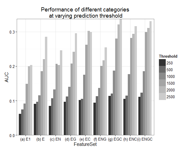
Figure 4: AUC versus Prediction Threshold

6.4 Comparison on Existing Datasets

To answer the third question, we experimented on the dataset of 595K users compiled by Weng et al. [35], made available on their website. We will refer to their dataset as WengDat. For our results to be directly comparable with Weng et al.’s approach on their dataset, we used their definition of virality, i.e., a hashtag is declared to be viral if it lies in the top $10\%$ of all the hashtags in a ranking based on the total number of tweets for each hashtag at the end of the observation period. We used their prediction threshold as used by them, i.e., $n=50$, and their learning setting as theirs i.e., Random Forests with 500 trees and 10 fold cross validation over a random split of the data. We did not perform any undersampling on this dataset. We compared our feature combinations with Weng et al.’s feature based approach. We refer to their approach as WFVP (Weng Feature based Virality Predictor). For WFVP, we directly use the results reported by them in their paper using their best combination of features.

Table 7 compares the performances of WFVP and CGNP using various feature combinations. Weng et al. already demonstrated the superior performance of their approach over a number of non-trivial baselines so we report their final results here. We do not have AUC numbers for WFVP as they are not reported by Weng et al. We did not have geography information for their dataset so we used CGNP with only the three feature groups E, N and C. First, note that as on TwitDat, adding sophisticated features to CGNP helps improve performance. The most improvement is obtained by adding conductance based features as was the case with TwitDat. Compared to WFVP, we are able to achieve a significantly high recall at the cost of a smaller loss in precision. In a scenario where it is important not to miss a potentially viral topic (as is the case with many of our motivating applications), obtaining a high recall becomes important. Note that overall, our precision-recall combination results in an F-measure which is 4.5% more than the best results reported by Weng et al. A more fine grained comparison with WFVP throws additional light. Using only evolution and network based features, CGNP performs worse than WFVP in terms of F-measure. We attribute this primarily to the community based features used by Weng et al. which have been shown to be quite effective for prediction. Significantly, once conductance based features are added, CGNP starts outperforming WFVP, even when we do not include network based features. Effectively, conductance is able to make-up for the lack of community based features for the task of virality prediction (and in fact, performs better). Further, we note that our conductance based features are local in the sense that they can be computed by examining the relevant portion of the network where the hashtag is currently diffusing and does not require the entire network to be taken into memory.

Algorithm	Precision	Recall	F-meas.	AUC
Random	10.00	50.0	16.66	10.0
CGNP(E1)	26.07	59.59	36.28	28.7
CGNP(E)	29.50	50.65	37.28	33.8
CGNP(E+N)	32.22	52.51	39.94	39.1
CGNP(E+C)	46.12	54.37	49.91	52.5
CGNP(E+N+C)	43.61	61.63	51.08	53.1
WFVP	66.00	36.00	46.58	-

Table 7: Results comparing CGNP using various feature combinations with WFVP on WengDat (all values in %)

6.5 Geographical Trends

We also evaluated the performance of CGNP over hashtags based on their spread within individual geographies, i.e., the graph of interest was restricted to the nodes lying within individual geographies in the dataset. In particular, we experimented with three different geographies, namely, London, India and Quito. Since the number of users across each geography varies, we appropriately scaled the prediction and virality thresholds for individual geographies. Virality threshold was maintained at 10 times the prediction threshold, in line with the ratio used for the entire dataset. The prediction threshold was hand tuned to ensure there was sufficient information in the data up to that point. Table 8 presents the details about number of active users (i.e. those who have tweeted at least once), prediction and virality thresholds, and % of viral hashtags for each of the above geographies. Table 9 presents the F-measure and AUC values for various feature combinations for each of the geographies. Note that since we are already within individual geographies, the feature category $G$ is absent in the combination. As seen in case of the full dataset, the performance increases with increasing sophistication in the feature set. For London and India, maximum benefit is obtained using the conductance based features. Network based features help improve this further. For Quito, network based features seem to give a larger gain. Best feature combination is still E+N+C.

Geogr-	# Active	Prediction	Virality	% of Viral
aphy	users	Threshold	Threshold	Hashtags
London	226906	150	1500	3.56
India	28935	100	1000	8.67
Quito	91871	50	500	3.14

Table 8: Individual Geography Statistics

	London		India		Quito
Algorithm	F	AUC	F	AUC	F	AUC
Random	6.7	3.6	14.8	8.7	5.9	3.1
CGNP(E1)	14.53	9.1	26.85	19.6	19.42	8.8
CGNP(E)	15.38	10.4	31.26	23.9	17.69	9.0
CGNP(E+N)	14.21	9.3	34.84	27.6	22.52	17.1
CGNP(E+C)	20.19	14.8	37.54	31.3	17.42	9.7
CGNP(E+N+C)	22.17	15.5	42.03	36.2	23.56	17.3

Table 9: Results on Individual Geographies.

7 Conclusions

In this work, we have carefully studied the effect of three different sets of feature categories, i.e., network based, geography based and conductance based, for the task of predicting hashtag virality in a large dataset. Our main contribution is a novel feature set that includes new features based on the network properties of the users tweeting a hashtag and the geographical information contained in their profiles and in their tweets. Building on the intuition that the spread of memes across communities is a critical discriminator of viral topics we have introduced a suite of conductance based features for the prediction task. We found that all our three feature categories (apart from the baseline evolution based features), have a significant impact on virality prediction, with conductance being the most effective. This justifies the intuition regarding the relationships of communities and virality and suggests that a more dynamic view of communities, centred around the diffusion pattern of individual hashtags, is more appropriate and effective for the prediction task. The fact that our feature set outperforms approaches relying on static communities detected in the network (such as the work of [35]) is doubly important in view of the fact that detecting static communities in the entire network is very expensive computationally at scale.

Future research directions include further investigating the use of our proposed feature sets for predicting spread of topics in individual geographies, more carefully examining the relative impact of community based and conductance based features and incorporating semantic features in our framework.

References

- [1] Pranay Agarwal. Prediction of trends in online social network. Master’s thesis, Indian Institute of Technology, Delhi, 2013.
- [2] Sinan Aral and Dylan Walker. Creating social contagion through viral product design: A randomized trial of peer influence in networks. Manag. Sci., 57(9):1623–1639, 2011.
- [3] Sebastien Ardon, Amitabha Bagchi, Anirban Mahanti, Amit Ruhela, Aaditeshwar Seth, Rudra Mohan Tripathy, and Sipat Triukose. Spatio-temporal and events based analysis of topic popularity in Twitter. In Proc. 22nd ACM Intl. Conf. on Information and Knowledge Management (CIKM 2013), pages 219–228. ACM, 2013.
- [4] Jonah Berger and Katherine L Milkman. What makes online content viral? J. Marketing Res., 49(2):192–205, 2012.
- [5] Peter Bright. How the london riots showed us two sides of social networking. Posted on http://arstechnica.com/, 11 August 2011, August 2011.
- [6] Justin Cheng, Lada A. Adamic, P. Alex Dow, Jon M. Kleinberg, and Jure Leskovec. Can cascades be predicted? In Proc. 23rd Intl. World Wide Web Conference (WWW ’14), pages 925–936, 2014.
- [7] F. Chierichetti, S. Lattanzi, and A Panconesi. Almost tight bounds for rumour spreading with conductance. In Proc. 42nd ACM Symp. on Theory of computing (STOC ’10), pages 399–408, 2010.
- [8] Jesse Davis and Mark Goadrich. The relationship between precision-recall and roc curves. In Proceedings of the 23rd international conference on Machine learning, pages 233–240. ACM, 2006.
- [9] Chris Drummond and Robert C. Holte. C4.5, class imbalance, and cost sensitivity: Why under-sampling beats over-sampling. In ICML Workshop on Learning from Imbalanced Datasets, pages 1–8, 2003.
- [10] R. Ghosh and K. Lerman. A framework for quantitative analysis of cascades on networks. In Proc. 4th ACM International Conference on Web search and data mining (WSDM ’11), pages 665–674, 2011.
- [11] David F. Gleich and C. Seshadhri. Vertex neighborhoods, low conductance cuts, and good seeds for local community methods. In Proc. 18th ACM SIGKDD Intl. Conf. on Knowledge Discovery and Data Mining (KDD ’12), pages 597–605, 2012.
- [12] Marco Guerini, Jacopo Staiano, and David Albanese. Exploring image virality in Google Plus. In Proc. ASE/IEEE Intl. Conference on Social Computing (SocialCom 2013), pages 671–678, 2013.
- [13] Marco Guerini, Carlo Strapparava, and Gözde Özbal. Exploring text virality in social networks. In Proc. Intl. AAAI Conf. on Weblogs and Social Media (ICWSM 2011), 2011.
- [14] Venkatesan Guruswami. Rapidly mixing Markov chains: A comparison of techniques. Available at: http://www.cs.cmu.edu/ venkatg/pubs/pubs.html, 2000.
- [15] Lars Kai Hansen, Adam Arvidsson, Finn Årup Nielsen, Elanor Colleoni, and Michael Etter. Good friends, bad news-affect and virality in twitter. In Future information technology, pages 34–43. Springer, 2011.
- [16] Steve Harenberg, Gonzalo Bello, L. Gjeltema, Stephen Ranshous, Jitendra Harlalka, Ramona Seay, Kanchana Padmanabhan, and Nagiza Samatova. Community detection in large-scale networks: a survey and empirical evaluation. WIREs Comput Stat, 6:426–439, 2014.
- [17] Maximilian Jenders, Gjergji Kasneci, and Felix Naumann. Analyzing and predicting viral tweets. In WWW (Companion Volume), pages 657–664, 2013.
- [18] M. R. Jerrum and A. J. Sinclair. Approximating the permanent. SIAM J. Comput., 18:1149–1178, 1989.
- [19] Maksim Kitsak, Lazaros K Gallos, Shlomo Havlin, Fredrik Liljeros, Lev Muchnik, H Eugene Stanley, and Hernán A Makse. Identification of influential spreaders in complex networks. Nature Phys., 6(11):888–893, 2010.
- [20] Juhi Kulshrestha, Farshad Kooti, Ashkan Nikravesh, and Krishna P. Gummadi. Geographic Dissection of the Twitter Network. In Proc. ICWSM 2012, 2012.
- [21] H. Kwak, C. Lee, H. Park, and S. Moon. What is Twitter, a social network or a news media? In Proc. 19th Intl. conference on World Wide Web (WWW ’10), pages 591–600, 2010.
- [22] Kristina Lerman and Tad Hogg. Using a model of social dynamics to predict popularity of news. In Proc. 19th Intl. conference on World Wide Web (WWW ’10), pages 621–630. ACM, 2010.
- [23] J. Leskovec, L. Backstrom, and J. Kleinberg. Meme-tracking and the dynamics of the news cycle. In Proc. KDD ’09, pages 497–506. ACM, 2009.
- [24] Jure Leskovec, Kevin J. Lang, and Michael W. Mahoney. Empirical comparison of algorithms for network community detection. In Proc. 19th Intl. Conf. on World Wide Web (WWW ’10), pages 631–640, 2010.
- [25] Zongyang Ma, Aixin Sun, and Gao Cong. On predicting the popularity of newly emerging hashtags in twitter. J. Assoc. Inf. Sci. Technol., 64(7):1399–1410, 2013.
- [26] J. McGee, J Caverlee, and Z. Cheng. Location prediction in social media based on tie strength. In Proc. 22nd ACM Intl. Conf. on Information and Knowledge Management (CIKM 2013), pages 459–468, 2013.
- [27] Seth A. Myers, Chenguang Zhu, and Jure Leskovec. Information diffusion and external influence in networks. In Proc. KDD ’12, pages 33–41, 2012.
- [28] Onook Oh, Manish Agrawal, and H Raghav Rao. Rumor and Communication in Asia in the Internet Age, chapter 8, pages 143–155. Taylor and Francis, 2013.
- [29] S Rajyalakshmi, Amitabha Bagchi, Soham Das, and Rudra M Tripathy. Topic diffusion and emergence of virality in social networks. arXiv preprint arXiv:1202.2215, 2012.
- [30] D. M. Romero, B. Meeder, and J. Kleinberg. Differences in the mechanics of information diffusion across topics: idioms, political hashtags, and complex contagion on twitter. In Proc. 20th Intl. conf. on World Wide Web (WWW ’11), pages 695–704, 2011.
- [31] Bongwon Suh, Lichan Hong, Peter Pirolli, and Ed H Chi. Want to be retweeted? large scale analytics on factors impacting retweet in twitter network. In IEEE/ASE SocialCom 2010, pages 177–184. IEEE, 2010.
- [32] Gabor Szabo and Bernardo A Huberman. Predicting the popularity of online content. Comm. ACM, 53(8):80–88, 2010.
- [33] Luam Catao Totti, Felipe Almeida Costa, Sandra Eliza Fontes de Avila, Eduardo Valle, Wagner Meira Jr., and Virgilio Almeida. The impact of visual attributes on online image diffusion. In Proc. ACM Web Science Conference (WebSci ’14), pages 42–51, 2014.
- [34] Lilian Weng, Alessandro Flammini, Alessandro Vespignani, and Filippo Menczer. Competition among memes in a world with limited attention. Sci. Rep., 2, 2012.
- [35] Lilian Weng, Filippo Menczer, and Yong-Yeol Ahn. Virality prediction and community structure in social networks. Sci. Rep., 3, 2013.
- [36] Lilian Weng, Filippo Menczer, and Yong-Yeol Ahn. Predicting successful memes using network and community structure. In 8th Intl. AAAI Conference on Weblogs and Social Media (ICWSM 2014), 2014.
- [37] Fang Wu and Bernardo A Huberman. Novelty and collective attention. Proc. Natl. Acad. Sci. U.S.A, 104(45):17599–17601, 2007.
- [38] T Zaman, E B Fox, and E T Bradlow. A bayesian approach for predicting the popularity of tweets. Ann. Appl. Stat., 8(3):1583–1611, 2014.