Formation of Rotational Discontinuities in Compressive three-dimensional MHD Turbulence

Abstract

Measurements of solar wind turbulence reveal the ubiquity of discontinuities. In this study, we investigate how the discontinuities, especially rotational discontinuities (RDs), are formed in magnetohydrodynamic (MHD) turbulence. In a simulation of the decaying compressive three-dimensional (3-D) MHD turbulence with an imposed uniform background magnetic field, we detect RDs with sharp field rotations and little variations of magnetic field intensity as well as mass density. At the same time, in the de Hoffman-Teller (HT) frame, the plasma velocity is nearly in agreement with the Alfvén speed, and is field-aligned on both sides of the discontinuity. We take one of the identified RDs to analyze in details its 3-D structure and temporal evolution. By checking the magnetic field and plasma parameters, we find that the identified RD evolves from the steepening of the Alfvén wave with moderate amplitude, and that steepening is caused by the nonuniformity of the Alfvén speed in the ambient turbulence.

1 INTRODUCTION

Since the beginning of the space age, the solar wind has been regarded as an excellent natural laboratory for studying the plasma turbulence. The endeavoring research over decades has revealed that the discontinuities are ubiquitous in the solar wind (Burlaga, 1969, 1971; Smith, 1973; Solodyna et al., 1977; Tsurutani & Smith, 1979; Neugebauer et al., 1984; Lepping & Behannon, 1986; Tsurutani et al., 1994, 1996; Lee et al., 1996; Horbury et al., 2001; Knetter et al., 2004; Tsurutani et al., 2005; Neugebauer, 2006; Vasquez et al., 2007; Li, 2008; Lin et al., 2009; Sonnerup et al., 2010; Teh et al., 2011; Haaland et al., 2012; Malaspina & Gosling, 2012; Wang et al., 2013; Paschmann et al., 2013). These discontinuities appear as large and rapid changes in properties of the plasma and magnetic field, and are identified as statically advected tangential discontinuities (TDs), or propagating rotational discontinuities (RDs). The TDs are characterized by small normal components of the magnetic field, large variations of magnetic field intensity and density jumps, while the RDs have large normal components of the magnetic field, but small variations of magnetic field intensity and density (Hudson, 1970).

By measurements of the magnetic field from Pioneer 6, Burlaga (1969) observed the discontinuities in the magnetic-field direction with special emphasis on their distribution in time. Based on interplanetary field measurements made by the vector helium magnetometers onboard Pioneer 10 and Pioneer 11, Tsurutani & Smith (1979) investigated a possible dependence of the occurrence rate and the properties of the discontinuities on radial distance between 1 and 8.5 AU. Lepping & Behannon (1986) surveyed the data from the Mariner 10 primary mission to study the characteristics of the discontinuities in the interplanetary magnetic field at heliographic distances of 1.0, 0.72, and 0.46 AU, and found an $r^{-1.3\pm 0.4}$ dependence for the daily average number of discontinuities per hour. With Ulysses magnetic field and plasma data obtained at radial distances ranging between 1 and 5 AU from the Sun and at high heliographic latitudes, Tsurutani et al. (1994) discovered two regions where the occurrence rate of interplanetary discontinuities is high: in stream-stream interaction regions and in Alfvén wave trains. To determine the normals of the discontinuities, Horbury et al. (2001) explored the discontinuities measured by three spacecraft WIND, IMP 8, and Geotail together with the solar wind velocity measured at Geotail, and obtained quite different distributions of the discontinuity types. With magnetic field data from the ACE spacecraft, Vasquez et al. (2007) extended the survey of discontinuity properties to small spread angles of the field vectors across the discontinuity, and found that solar wind discontinuities are far more abundant at small than at large spread angles. By measurements from the WIND spacecraft, Wang et al. (2013) studied the intermittent structures in solar wind turbulence, which are identified as being mostly rotational discontinuities (RDs) and rarely tangential discontinuities (TDs) based on the technique described by Smith (1973) and Tsurutani & Smith (1979). Paschmann et al. (2013) carried out a comprehensive study of directional discontinuties and Alfvénic fluctuations in the solar wind on the basis of Cluster data.

So far, there are still debates regarding the origin and nature of the discontinuities in the solar wind. Since RDs appear as a compressed Alfvén wave, nonlinear wave steepening has been suggested as the cause of its formation (Cohen & Kulsrud, 1974; Malara & Elaoufir, 1991; Tsurutani et al., 1994; Vasquez & Hollweg, 1996, 1998a, 1998b; Tsurutani et al., 2002; Marsch & Verscharen, 2011). By numerically calculating the evolution of an initially parallel-propagating, elliptically polarized wave train in a cold plasma, Cohen & Kulsrud (1974) were the first to investigate this possibility, and showed that this wave evolves to a constant-B solution with RDs that rotate the field by exactly $180^{\circ}$. Vasquez & Hollweg (1996) continued this study, but conducted a 1.5-D hybrid numerical simulation study of the evolution of obliquely propagating, linearly polarized Alfvén wave trains. They found that large-amplitude $dB/B_{0}>1$ wave trains steepen and produce RDs which always rotate the field by $<180^{\circ}$. Vasquez & Hollweg (1998a) also presented 2.5-D numerical simulations of a small group of nonplanar Alfvén waves to show the generation of imbedded RDs. It should be noted that in their models the formation of RDs probably occurs relatively near the Sun where most Alfvénic fluctuations originate.

There is another model suggesting that MHD turbulence dynamically generates these discontinuities as the solar wind flows outward. Recently, numerical simulations have been done to investigate this assertion (Greco et al., 2008, 2009, 2010; Servidio et al., 2011; Zhdankin et al., 2012a, b). Through analyses of MHD simulation data, Greco et al. (2008) examined the relationship between discontinuities identified by classical methods, and coherent structures identified by using intermittency statistics. They found that the two methods produce remarkably similar distributions of waiting times, and in fact identify many of the same events. Greco et al. (2009) further examined the link between intermittent turbulence and MHD discontinuities, directly comparing simulations of MHD turbulence with statistical analysis from ACE solar wind data. Their results support the notion that some solar wind discontinuities are consequences of intermittent turbulence. In direct numerical simulations of MHD turbulence with an imposed uniform magnetic field, Zhdankin et al. (2012a) investigated the statistical properties of magnetic discontinuities, and concluded that the discontinuities observed in the solar wind can be reproduced by MHD turbulence. However, these works conducted statistical studies, and did not give a clear illustration of how discontinuities, especially RDs, are formed in MHD turbulence.

In the present study, we utilize a compressible 3-D MHD model to illustrate and analyze the forming of RDs in the turbulence. By checking the magnetic field and plasma properties, it is found that RD is produced by the steepening of a moderate-amplitude Alfvén wave with nonuniform propagating speed. The paper is organized as follows. In Section 2, a general description of the numerical MHD model is given. Section 3 describes the results of the numerical simulation and its analysis. Section 4 is reserved for the summary and discussion.

2 NUMERICAL MHD MODEL

The description of the plasma is given by compressible 3-D MHD, which involves a fluctuating flow velocity $\mathbf{v}(x,y,z,t)$, magnetic field $\mathbf{b}(x,y,z,t)$, density $\rho(x,y,z,t)$, and temperature $T(x,y,z,t)$. An uniform guide field $B_{0}$ is assumed in the $z-$direction, so the total magnetic field is $\mathbf{B}=\mathbf{B_{0}}+\mathbf{b}$.

The MHD equations are written in the following non-dimensional form:

$$\frac{\partial\rho}{\partial t}+\nabla\cdot\rho\mathbf{u}=0\ ,$$ (1)

$$\frac{\partial\rho\mathbf{u}}{\partial t}+\nabla\cdot\left[\rho\mathbf{u}\mathbf{u}+(p+\frac{1}{2}\mathbf{B}^{2})\mathbf{I}-\mathbf{B}\mathbf{B}\right]=0\ ,$$ (2)

$$\frac{\partial e}{\partial t}+\nabla\cdot\left[\mathbf{u}(e+p+\frac{1}{2}\mathbf{B}^{2})-(\mathbf{u}\cdot\mathbf{B})\mathbf{B}\right]=\nabla\cdot(\mathbf{B}\times\eta\mathbf{j}),$$ (3)

$$\frac{\partial\mathbf{B}}{\partial t}+\nabla\cdot(\mathbf{u}\mathbf{B}-\mathbf{B}\mathbf{u})=\eta\nabla^{2}\mathbf{B}\ ,$$ (4)

where

$$e=\frac{1}{2}\rho\mathbf{u}^{2}+\frac{p}{\gamma-1}+\frac{1}{2}\mathbf{B}^{2},\ \ \ \ \mathbf{j}=\nabla\times\mathbf{B},$$ (5)

which corresponds to the total energy density and current density, respectively. Here, $\rho$ is the mass density; $\mathbf{u}=(v_{x},v_{y},v_{z})$ are the $x$, $y$, and $z-$components of velocity; $p$ is the thermal pressure; $\mathbf{B}$ denotes the magnetic field; $t$ is time; $\gamma=5/3$ is the adiabatic index; and $\eta$ is the magnetic resistivity.

Three independent parameters, an initial mean density $\rho_{0}$, a characteristic length $L$, and a characteristic plasma speed $v_{0}=\delta b/\sqrt{4\pi\rho_{0}}$ with $\delta b=\langle b^{2}\rangle^{1/2}$, are used to normalize the MHD equations. Other variables are normalized by their combinations. The dimensionless numbers appearing in the equations are the Mach number $M_{s}=v_{0}/c_{s}$, where $c_{s}=\sqrt{\gamma p_{0}/\rho_{0}}$ is the sound speed, and the magnetic Reynolds number $R_{m}=v_{0}L/\eta$. Here, we take $M_{s}$ to be 0.5, consistent with the solar wind observations at 1 AU, and $R_{m}$ to be 1000, which is limited by the available spatial resolution. The uniform guide field $B_{0}$ is two times of the fluctuating field $\mid\delta\mathbf{b}\mid$.

We consider periodic boundary conditions in a cube with a side length of $2\pi L$ and a resolution defined by the number of grid points which is $512^{3}$, and run a simulation from an initial state with kinetic and magnetic energy per unit mass $\langle v^{2}\rangle=\langle b^{2}\rangle=1$. The fluctuations initially populate an annulus in the Fourier $k-$space such that $1\leq k\leq 8$, with constant amplitude and random phases (Matthaeus et al., 1996; Dmitruk et al., 2004). The initial normalized cross helicity is set to be 0.9 such that the primordial fluctuations are highly Alfvénic. The initial density and thermal pressure are set to be uniform.

To solve the equations, we employ a splitting-based finite-volume numerical scheme. The fluid part is solved by the Godunov-type central scheme and the magnetic part by the constrained transport approach, in conjunction with the method called second-order Monotone Upstream Schemes for Conservation Laws (MUSCL) for reconstruction and with the approximate Riemann solvers of Harten-Lax-van Leer (HLL) for calculation of the numerical fluxes (Feng et al., 2011). The explicit second-order Runge-Kutta stepping with total variation diminishing is applied in time integration.

3 NUMERICAL RESULTS

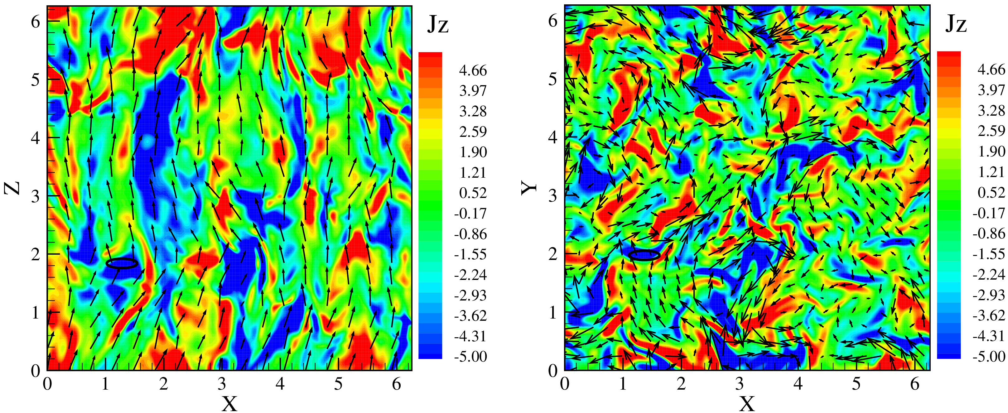
Figure 1: Distribution of the $z-$component of the current density $J_{z}$ in an $x$-$z$ (Left) and $x$-$y$ (Right) plane at $t=1.25$. Superposed by arrows are the projections of the magnetic field vectors in the $x$-$z$ (Left) and the $x$-$y$ plane (Right). The black ellipses mark the region where the identified RD is formed.

Figure 1 shows the distribution of the current density in the $z-$direction $J_{z}$ in the $x$-$z$ (Left) and $x$-$y$ (Right) plane at $t=1.25$. The arrows superposed on the images are the projections of the magnetic field vectors in the $x$-$z$ (Left) and the $x$-$y$ plane (Right). The black ellipses mark the region where the identified RD is formed. From this figure, we can see that a large-scale background magnetic field is clearly present in the $z-$direction. As a result of the well-known anisotropic behavior of magnetic field fluctuations in MHD with an imposed uniform guide field (Matthaeus et al., 1996), current density structures preferentially align along the guide field direction, as shown in the left panel, and become much more varying in the perpendicular cross section, as shown in the right panel. Also, $J_{z}$ appears to be large in magnitude at the location where the identified RD is formed.

In order to detect RD, we first seek the regions with large normalized partial variance of increments (PVI) of the magnetic field vector. PVI in 3-D space is defined as

$$\mbox{PVI}(x,y,z)=\frac{\mid\mathbf{B}(x+\Delta x,y+\Delta y,z+\Delta z)-\mathbf{B}(x-\Delta x,y-\Delta y,z-\Delta z)\mid}{\sqrt{\langle\mid\mathbf{B}(x+\Delta x,y+\Delta y,z+\Delta z)-\mathbf{B}(x-\Delta x,y-\Delta y,z-\Delta z)\mid^{2}\rangle}}$$

where $\Delta x,\ \Delta y$ and $\Delta z$ is the grid increment in the $x-$, $y-$ and $z-$direction, respectively. We first sample the magnetic field $\mathbf{B}$, plasma velocity $\mathbf{v}$, density $\rho$, and temperature $T$ along a linear path through the region with $\mbox{PVI}>2$, and then perform along that path the minimum variance analysis (MVA) (Sonnerup & Cahill, 1967) using the magnetic field data to find the maximum variance direction ($L$), intermediate variance direction ($M$), minimum variance direction ($N$), and their corresponding eigenvalues $\lambda_{1}$, $\lambda_{2}$, and $\lambda_{3}$. Finally, we check the 3-D plasma and field structure of the possible events.

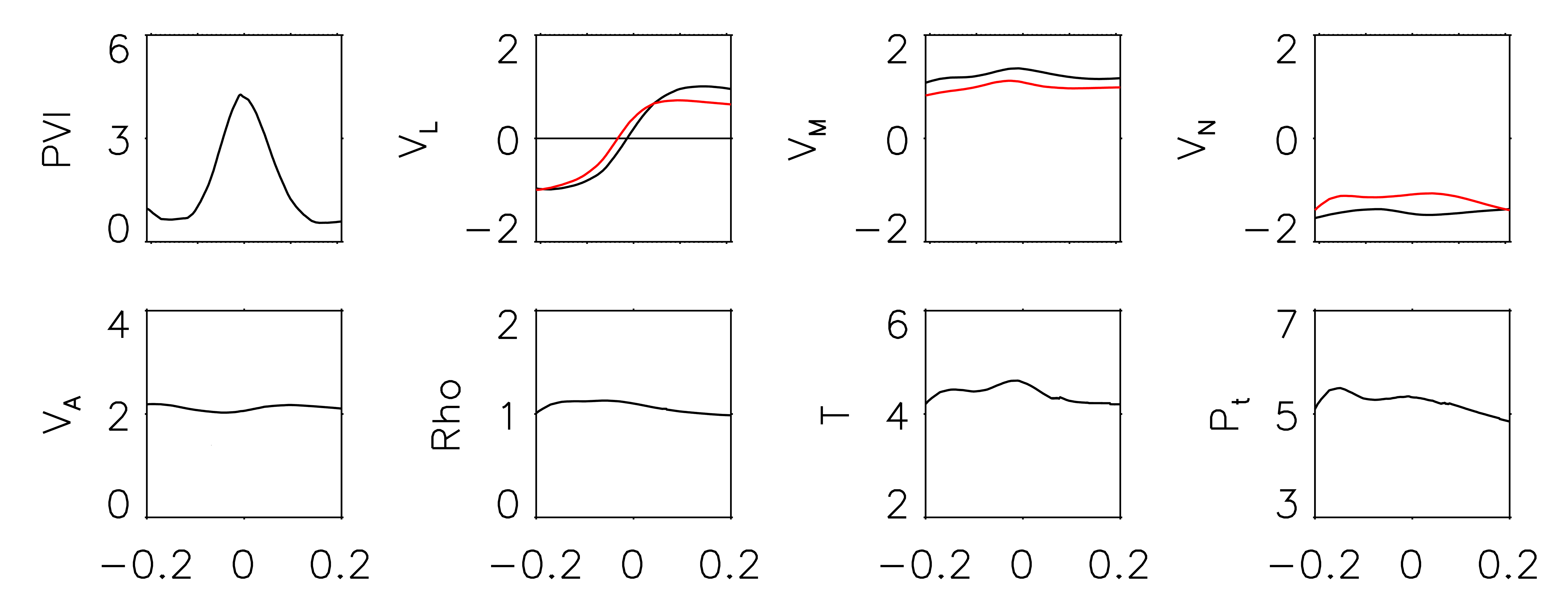
Figure 2: Magnetic field and plasma parameters along the sampling interval for an identified RD. $V_{L}$, $V_{M}$, and $V_{N}$ denote the $L,M,N$ components of the Alfvén velocity (black lines) and plasma velocity (red lines) respectively as derived from minimum variance analysis (MVA). The Horizontal axis displays the coordinate $s$ along the sampling path, with $s=0$ at the RD point.

Figure 2 shows the magnetic field and plasma parameters along the sampling interval for an identified RD. In this figure, the magnetic field has been converted into the Alfvén velocity $\mathbf{V_{A}}$, by using $\mathbf{V_{A}}=\mathbf{B}/\sqrt{\rho}$ . We can see that the sampling series of PVI is rather close to 0, except near the center. The large jumps of the Alfvén velocity and plasma velocity mainly occur along the $L$ direction, with $V_{L}$ jumping from -1.0 to 1.0. The $N-$components $V_{N}$ of them are nearly constant, and are equal to 1.6, along with a nearly negligible jump of $\mid\mathbf{V_{A}}\mid$, the magnitude of Alfvén speed. Also, the Alfvén speed and plasma speed are nearly in agreement over the entire interval, including the jump across the RD itself. The positive correlation between them implies the RD propagation anti-parallel to the magnetic field. The density $\rho$, temperature $T$ and total pressure $P_{t}$ (which consists of the summed magnetic pressure and thermal pressure) all exhibit relatively constant traces throughout the interval. To be noted, the jump of $V_{L}$ and the large value of $V_{N}$, together with the relatively slight change of $P_{t}$ as well as $\rho$, corroborate that this event is a RD.

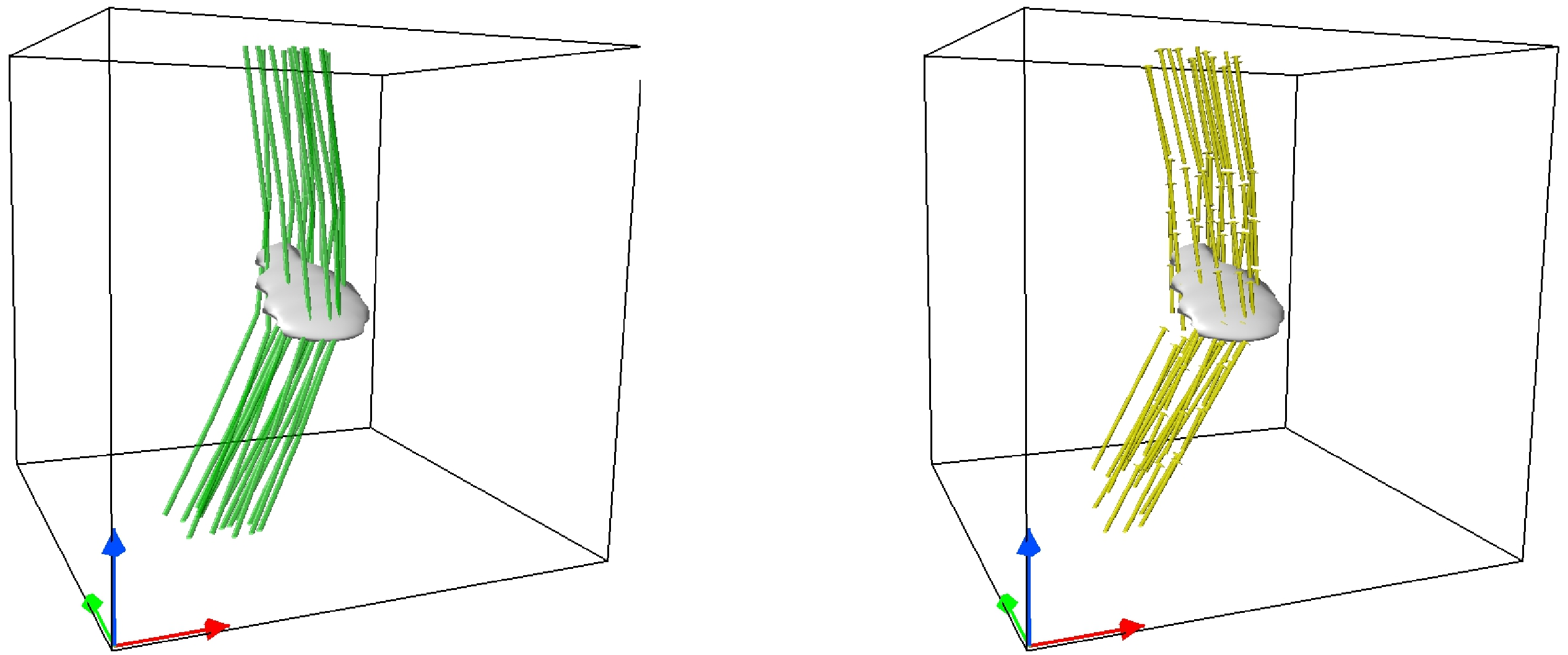
Figure 3: Three-dimensional structure of the identified RD. The green lines in the left panel denote magnetic field lines and the yellow arrows in the right panel are plasma velocity vectors, which are converted into de Hoffman-Teller (HT) frame. The light gray surface is the isosurface where $\mbox{PVI}=4$, showing the RD, and red, green as well as blue arrows display the $x-$, $y-$, and $z-$direction, respectively.

Figure 3 exhibits the 3-D structure of the identified RD. The green lines in the left panel denote magnetic field lines and the yellow arrows in the right panel are plasma velocity vectors, which are converted into the de Hoffman-Teller (HT) frame. The light gray surface is the isosurface where $\mbox{PVI}=4$, showing RD, and red, green as well as blue arrows display the $x-$, $y-$, and $z-$direction, respectively. This figure displays that in the HT frame, magnetic field and plasma velocity have evident normal components across the RD, and they both rotate by a certain angle. Also, the plasma velocity is field aligned on both sides of the discontinuity, in accordance with the Alfvénic nature of RD. The identified RD appears as a thin surface and its normal inclines to the $z-$axis.

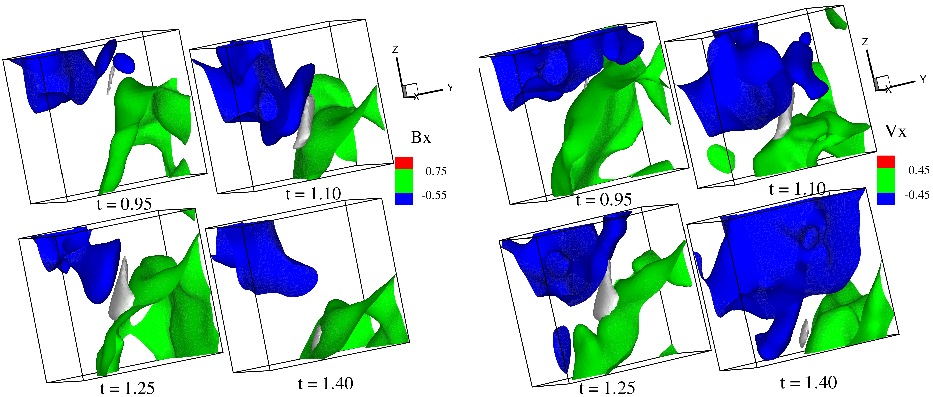
Figure 4: The isosurfaces of $B_{x}$ (Left) and $V_{x}$ (Right) at different moments in time, with the light gray surface being the isosurface where $\mbox{PVI}=3$, and exhibiting the identified RD.

To see how the identified RD is formed, Figure 4 shows the isosurfaces of $B_{x}$ (Left) and $V_{x}$ (Right) at different moments in time. These isosurfaces are associated with the Alfvén wave as shown below. $\mbox{PVI}=3$ is used here to exhibit the identified RD at these four moments, and is shown as the light gray surface. From this figure, it is notable that the mutual approaching of the two isosurfaces of $B_{x}$ ($V_{x}$), which describes the steepening of the Alfvén wave, leads to the formation of a RD. At $t=0.95$, the isosurface with $B_{x}=-0.55$ ($V_{x}=-0.45$) is relatively away from the isosurface with $B_{x}=0.75$ ($V_{x}=0.45$), and the transition of $B_{x}$ ($V_{x}$) from $B_{x}=-0.55$ ($V_{x}=-0.45$) to $B_{x}=0.75$ ($V_{x}=0.45$) is gentle. The isosurface where $\mbox{PVI}=3$ is small and thin. At $t=1.10$, the isosurfaces with $B_{x}=-0.55$ ($V_{x}=-0.45$) and $B_{x}=0.75$ ($V_{x}=0.45$) approach each other, and the transition between the two isosurfaces of $B_{x}$ ($V_{x}$) becomes steep. Correspondingly, the isosurface where $\mbox{PVI}=3$ grows. Afterwards, that is at $t=1.25$, the two isosurfaces of $B_{x}$ ($V_{x}$) are close enough to each other, and the transition between the two isosurfaces of $B_{x}$ ($V_{x}$) becomes steeper. The isosurface where $\mbox{PVI}=3$ grows larger and thicker, and the identified RD is fully grown. However, at $t=1.40$, the isosurfaces with $B_{x}=-0.55$ ($V_{x}=-0.45$) is far away from the isosurface with $B_{x}=0.75$ ($V_{x}=0.45$), and the transition between the two isosurfaces of $B_{x}$ ($V_{x}$) becomes gentle again. As a result, the isosurface where $\mbox{PVI}=3$ becomes small and thin. The identified RD starts to collapse.

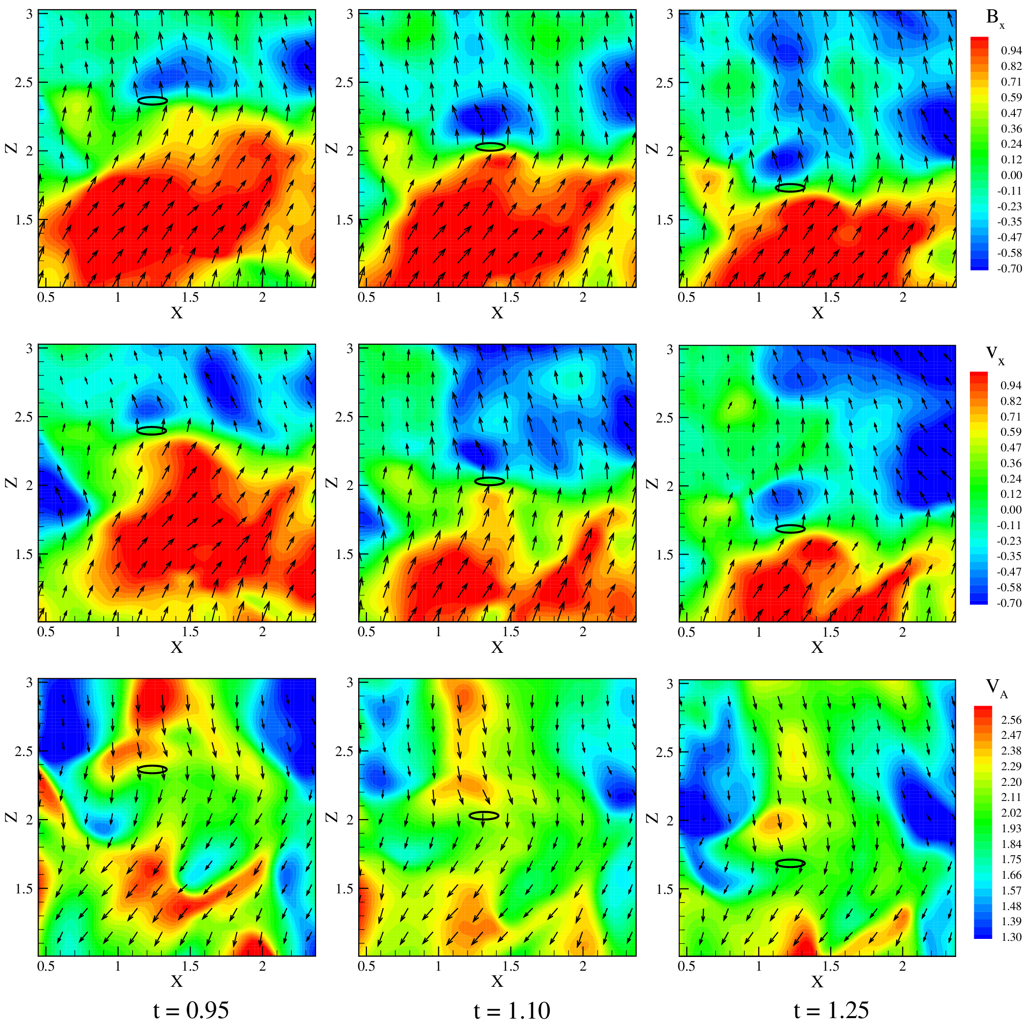
Figure 5: Distribution of $B_{x}$ (the first row), $V_{x}$ (the second row), and $V_{A}$ (the third row) in a subzone of the $x$-$z$ plane (which passes through the identified RD) at different moments in time. Superposed by arrows are the projections of the magnetic field (the first row), velocity field in the HT frame (the second row), and negative Alfvén speed field (the third row) vectors in the $x$-$z$ plane. The black ellipses mark the position where the identified RD is formed.

To understand the type of waves before the RD is formed and to investigate the process of the evolution of the isosurfaces mentioned above, Figure 5 exhibits the distribution of $B_{x}$ (the first row), $V_{x}$ (the second row), and $V_{A}$ (the third row) in the neighborhood of the identified RD in the plane $x$-$z$ at different moments in time. Superposed by arrows are the projections of the magnetic field (the first row), velocity field in the HT frame (the second row), and negative Alfvén speed field (the third row) vectors in the $x$-$z$ plane. The black ellipses mark the position where the identified RD is formed. Near the ellipses, the magnitudes of $B_{x}$ and $V_{x}$ are almost same (they are set to have the same color scales so that the same color stands for the same value), and the directions of the in-plane projection of the $\mathbf{B}$ and $\mathbf{V}$ vectors are almost identical. Hence in this vicinity, we have $\mathbf{V}=\mathbf{B}/\sqrt{\rho_{0}}$ (we recall that $\rho_{0}\approx 1$), which agrees with the polarity relations of an Alfvén wave. In other words, the RD is detected in a neighbouring Alfvénic environment that apparently favours RD formation.

Therefore, $V_{A}$ can be regarded as the propagation velocity of the structures relative to the location where the RD forms. Hence it is significant to trace the changes of the Alfvén speed. In the third row in Figure 5 where the evolution of the Alfvén speed is shown, we can see that at $t=0.95$, there is a difference of Alfvén speed across the black ellipse, which makes the layers with negative $B_{x}$ (blue in Figure 4), propagate faster than that with positive $B_{x}$ (green in Figure 4). At $t=1.10$, there is the evidence for approaching and squeezing of these two layers. The difference of Alfvén speed there remains. This will drive these two layers further to approach each other. At $t=1.25$, their transition becomes sharp, and the difference of Alfvén speed nearly disappears. This status continues until $t=1.40$, when the transition becomes gentle as a result of the faster propagation of the layers with positive $B_{x}$ than that with negative $B_{x}$. It is obvious that the difference of Alfvén speed makes the Alfvén wave steepen, a process which forms the identified RD.

4 SUMMARY AND DISCUSSION

In this study, we use a simulation of the decaying compressive 3-D MHD turbulence with an imposed uniform guide field as a test case to explore the formation of RDs in MHD turbulence. Motivated by solar wind observation at 1 AU, we consider a moderate fluctuation amplitude corresponding to $\delta b/B_{0}=0.5$ and high Alfvénic correlations with the normalized cross helicity initially of 0.9. A case study is thus conducted to illustrate the origin of RDs in MHD turbulence.

The numerical simulation shows the well-known anisotropic behavior of the turbulent MHD field, with the current density structures preferentially aligning along the guide field direction and scattering in the perpendicular plane. To detect the RDs in this simulated magnetofluid, we first seek the regions with large PVI, then conduct a MVA by sampling the parameters along a linear path, and finally check the 3-D structure of the possible RD events. One clear RD is identified with sharp field rotations and little variations of the magnetic field intensity as well as density. At the same time, in the HT frame, the plasma velocity is nearly in agreement with the Alfvén speed, and is field aligned on both sides of the discontinuity, satisfying the Walen relation that expresses the Alfvénic nature of an RD. The normal direction of the identified RD inclines to the $z-$axis, and propagates anti-parallel to the guide field.

The comprehensive information obtained by the simulation of the magnetic field and plasma parameters associated with the RD implies that the RD is produced by the steepening of the moderate-amplitude Alfvén wave with nonuniform Alfvén speed in the ambient turbulence. Before the RD is formed, the layers with negative $B_{x}$ smoothly transits to the layers with positive $B_{x}$. However, there is a difference of Alfvén speed across them, which makes the layers with negative $B_{x}$ chase after its counterpart with positive $B_{x}$. As they are driven by the neigbouring turbulence to approach and squeeze each other, the transition between them undergoes further steepening until the difference of Alfvén speed nearly disappears. At the same time, the identified RD is formed.

In this work we investigated only one RD. Certainly, there are many RDs generated in the simulation of decaying MHD turbulence. It will be worthwhile to conduct statistical studies to see whether all RDs are produced by this nonlinear steepening of an Alfvén wave. Meanwhile, TDs are also formed. It can be inspiring to investigate their generation mechanism in MHD turbulence. Furthermore, the parameters we adopted in the simulation (e.g. Mach number, cross helicity, plasma $\beta$) may influence the forming of RDs or TDs. In the future, we plan to conduct a parameter study to investigate the possible effects induced by parameter variation on the generation of discontinuties in MHD turbulence.

References

- Burlaga (1969) Burlaga, L. F. 1969, Sol. Phys., 7, 54
- Burlaga (1971) —. 1971, J. Geophys. Res., 76, 4360
- Cohen & Kulsrud (1974) Cohen, R. H. & Kulsrud, R. M. 1974, Physics of Fluids, 17, 2215
- Dmitruk et al. (2004) Dmitruk, P., Matthaeus, W. H., & Seenu, N. 2004, ApJ, 617, 667
- Feng et al. (2011) Feng, X., Zhang, S., Xiang, C., Yang, L., Jiang, C., & Wu, S. T. 2011, ApJ, 734, 50
- Greco et al. (2008) Greco, A., Chuychai, P., Matthaeus, W. H., Servidio, S., & Dmitruk, P. 2008, Geophys. Res. Lett., 35, 19111
- Greco et al. (2009) Greco, A., Matthaeus, W. H., Servidio, S., Chuychai, P., & Dmitruk, P. 2009, ApJ, 691, L111
- Greco et al. (2010) Greco, A., Servidio, S., Matthaeus, W. H., & Dmitruk, P. 2010, Planet. Space Sci., 58, 1895
- Haaland et al. (2012) Haaland, S., Sonnerup, B., & Paschmann, G. 2012, Annales Geophysicae, 30, 867
- Horbury et al. (2001) Horbury, T. S., Burgess, D., Fränz, M., & Owen, C. J. 2001, Geophys. Res. Lett., 28, 677
- Hudson (1970) Hudson, P. D. 1970, Planet. Space Sci., 18, 1611
- Knetter et al. (2004) Knetter, T., Neubauer, F. M., Horbury, T., & Balogh, A. 2004, J. Geophys. Res., 109, 6102
- Lee et al. (1996) Lee, L. C., Lin, Y., & Choe, G. S. 1996, Sol. Phys., 163, 335
- Lepping & Behannon (1986) Lepping, R. P. & Behannon, K. W. 1986, J. Geophys. Res., 91, 8725
- Li (2008) Li, G. 2008, ApJ, 672, L65
- Lin et al. (2009) Lin, C. C., Tsai, C. L., Chen, H. J., Weng, C. J., Chao, J. K., & Lee, L. C. 2009, J. Geophys. Res., 114, 8102
- Malara & Elaoufir (1991) Malara, F. & Elaoufir, J. 1991, J. Geophys. Res., 96, 7641
- Malaspina & Gosling (2012) Malaspina, D. M. & Gosling, J. T. 2012, J. Geophys. Res., 117, n/a
- Marsch & Verscharen (2011) Marsch, E. & Verscharen, D. 2011, Journal of Plasma Physics, 77, 385
- Matthaeus et al. (1996) Matthaeus, W. H., Ghosh, S., Oughton, S., & Roberts, D. A. 1996, J. Geophys. Res., 101, 7619
- Neugebauer (2006) Neugebauer, M. 2006, J. Geophys. Res., 111, 4103
- Neugebauer et al. (1984) Neugebauer, M., Clay, D. R., Goldstein, B. E., Tsurutani, B. T., & Zwickl, R. D. 1984, J. Geophys. Res., 89, 5395
- Paschmann et al. (2013) Paschmann, G., Haaland, S., Sonnerup, B., & Knetter, T. 2013, Annales Geophysicae, 31, 871
- Servidio et al. (2011) Servidio, S., Greco, A., Matthaeus, W. H., Osman, K. T., & Dmitruk, P. 2011, J. Geophys. Res., 116, 9102
- Smith (1973) Smith, E. J. 1973, J. Geophys. Res., 78, 2054
- Solodyna et al. (1977) Solodyna, C. V., Belcher, J. W., & Sari, J. W. 1977, J. Geophys. Res., 82, 10
- Sonnerup & Cahill (1967) Sonnerup, B. U. O. & Cahill, Jr., L. J. 1967, J. Geophys. Res., 72, 171
- Sonnerup et al. (2010) Sonnerup, B. U. Ö., Haaland, S. E., & Paschmann, G. 2010, Annales Geophysicae, 28, 1229
- Teh et al. (2011) Teh, W.-L., Sonnerup, B. U. Ö., Paschmann, G., & Haaland, S. E. 2011, J. Geophys. Res., 116, 4105
- Tsurutani et al. (2002) Tsurutani, B. T., Dasgupta, B., Galvan, C., Neugebauer, M., Lakhina, G. S., Arballo, J. K., Winterhalter, D., Goldstein, B. E., & Buti, B. 2002, Geophys. Res. Lett., 29, 86
- Tsurutani et al. (2005) Tsurutani, B. T., Guarnieri, F. L., Lakhina, G. S., & Hada, T. 2005, Geophys. Res. Lett., 32, 10103
- Tsurutani et al. (1996) Tsurutani, B. T., Ho, C. M., Arballo, J. K., Smith, E. L., Goldstein, B. E., Neugebauer, M., Balogh, A., & Feldman, W. C. 1996, J. Geophys. Res., 101, 11027
- Tsurutani et al. (1994) Tsurutani, B. T., Ho, C. M., Smith, E. J., Neugebauer, M., Goldstein, B. E., Mok, J. S., Arballo, J. K., Balogh, A., Southwood, D. J., & Feldman, W. C. 1994, Geophys. Res. Lett., 21, 2267
- Tsurutani & Smith (1979) Tsurutani, B. T. & Smith, E. J. 1979, J. Geophys. Res., 84, 2773
- Vasquez et al. (2007) Vasquez, B. J., Abramenko, V. I., Haggerty, D. K., & Smith, C. W. 2007, J. Geophys. Res., 112, 11102
- Vasquez & Hollweg (1996) Vasquez, B. J. & Hollweg, J. V. 1996, J. Geophys. Res., 101, 13527
- Vasquez & Hollweg (1998a) —. 1998a, J. Geophys. Res., 103, 349
- Vasquez & Hollweg (1998b) —. 1998b, J. Geophys. Res., 103, 335
- Wang et al. (2013) Wang, X., Tu, C., He, J., Marsch, E., & Wang, L. 2013, The Astrophysical Journal Letters, 772, L14
- Zhdankin et al. (2012a) Zhdankin, V., Boldyrev, S., & Mason, J. 2012a, ApJ, 760, L22
- Zhdankin et al. (2012b) Zhdankin, V., Boldyrev, S., Mason, J., & Perez, J. C. 2012b, Phys. Rev. Lett., 108, 175004