Valley coupling in finite-length metallic single-wall carbon nanotubes

Abstract

Degeneracy of discrete energy levels of finite-length, metallic single-wall carbon nanotubes depends on type of nanotubes, boundary condition, length of nanotubes and spin-orbit interaction. Metal-1 nanotubes, in which two non-equivalent valleys in the Brillouin zone have different orbital angular momenta with respect to the tube axis, exhibits nearly fourfold degeneracy and small lift of the degeneracy by the spin-orbit interaction reflecting the decoupling of two valleys in the eigenfunctions. In metal-2 nanotubes, in which the two valleys have the same orbital angular momentum, vernier-scale-like spectra appear for boundaries of orthogonal-shaped edge or cap-termination reflecting the strong valley coupling and the asymmetric velocities of the Dirac states. Lift of the fourfold degeneracy by parity splitting overcomes the spin-orbit interaction in shorter nanotubes with a so-called minimal boundary. Slowly decaying evanescent modes appear in the energy gap induced by the curvature of nanotube surface. Effective one-dimensional model reveals the role of boundary on the valley coupling in the eigenfunctions.

I Introduction

Metallic single-wall carbon nanotubes (m-SWNTs) are ideal one-dimensional (1D) conductors of nanometer to micrometer length. Due to the confinement in the finite-length, energy levels of electrons are quantized and the eigenfunctions show standing wave behavior. Venema et al. (1999); Lemay et al. (2001) Fourfold degeneracy of the discrete energy levels observed in the tunneling spectroscopy measurements has been considered as an intrinsic property of SWNTs reflecting the two non-equivalent, degenerate valleys at the $K$ and $K^{\prime}$ points in the two-dimensional (2D) Brillouin zone (BZ) together with two spins degrees of freedom. Liang et al. (2002); Cobden and Nygård (2002); Jarillo-Herrero et al. (2005a); Moriyama et al. (2005); Sapmaz et al. (2005); Maki et al. (2005); Cao et al. (2005); Makarovski et al. (2006); Moriyama et al. (2007); Holm et al. (2008) Recent measurements with ultraclean SWNTs have found fine structures of the order of sub-milli-electron-volt in tunneling conductance spectra caused by spin-orbit interaction, Kuemmeth et al. (2008); Jhang et al. (2010); Jespersen et al. (2011); Steele et al. (2013) which lifts the fourfold degeneracy by spin splitting in each valley. Ando (2000); Chico et al. (2004); Huertas-Hernando et al. (2006); Chico et al. (2009); Izumida et al. (2009); Jeong and Lee (2009) On the other hand, some experiments show degeneracy behaviors other than above, such as gate-dependent oscillation of twofold and fourfold degeneracy, Maki et al. (2005); Makarovski et al. (2006); Moriyama et al. (2007); Holm et al. (2008) and many of them have been owed to extrinsic effects such as impurities.

In our previous study, Izumida et al. (2012) we pointed out the asymmetric velocities in the same valley for the m-SWNTs because of the curvature of nanotube surface. That is, the left- and right-going waves in the same valley have different velocities, $v_{\rm L}^{(K)}>v_{\rm R}^{(K)}(>0)$, where $v_{\rm L}^{(K)}$ ($v_{\rm R}^{(K)}$) is the velocity of left-going (right-going) wave at the $K$ valley, and we have the relations $v_{\rm L}^{(K)}=v_{\rm R}^{(K^{\prime})}$ and $v_{\rm L}^{(K^{\prime})}=v_{\rm R}^{(K)}$ because of the time-reversal symmetry. At the same time, we claimed the formation of vernier-scale-like energy spectrum, in which two sets of the energy levels with a constant energy separation between the levels have a similar but not-exactly the same separation for each set, if the strong valley coupling occurs, in which each set of the wavefunction is formed from a left-going wave at one valley and a right-going wave at another valley. As the result of the quantization of the wavenumber in the axis direction, there are two different sets of equi-spaced discrete energy levels, $\hbar v_{\rm L}^{(K)}\pi/L_{\rm NT}$ and $\hbar v_{\rm R}^{(K)}\pi/L_{\rm NT}$, like the vernier scale, Izumida et al. (2012) showing two- and fourfold oscillations as observed in the experiments, Maki et al. (2005); Makarovski et al. (2006); Moriyama et al. (2007); Holm et al. (2008) where $L_{\rm NT}$ is the nanotube length. On the other hand, for the case of valley decoupling, in which each wavefunction is formed from a left- and right-going waves in the same valley, the fourfold degeneracy and its lift by the spin-orbit interaction Ando (2000); Chico et al. (2004); Huertas-Hernando et al. (2006); Chico et al. (2009); Izumida et al. (2009); Jeong and Lee (2009) would be observed. Thus, it is important to reveal the coupling of the two valleys as a function SWNT chirality or the boundary shape for understanding the degeneracy behavior.

As is known that the particle-in-a-1D-box model cannot be directly applied to the m-SWNTs because there are two left-going waves and two right-going waves, in general, the ratios of these traveling waves in a standing wave are determined by microscopic conditions such as the chirality and the boundary condition. Previous calculations have shown the standing waves oscillating in the length scale of carbon-carbon bond for the armchair nanotubes, in which each standing wave is constructed in the condition of strong valley coupling. Rubio et al. (1999); Yaguchi and Ando (2001) On the other hand for the zigzag nanotubes, the slowly oscillating standing waves for doubly degenerate levels can be constructed in the condition of valley decoupling. Bulusheva et al. (1998); Rocha et al. (2002) The SWNTs have been classified in terms of the boundary condition. Using generalized parameters, McCann and Fal’ko classified the boundary conditions for the Dirac electrons in the m-SWNTs. McCann and Fal’ko (2004) By employing microscopic analysis on the boundary modes for the honeycomb lattice, Akhmerov and Beenakker showed that, except for the armchair edge, zigzag-type boundary condition Brey and Fertig (2006), in which two valleys decouple each other in the eigenfunctions, is applicable for general boundary orientation with a so-called minimal boundary, in which the edge has minimum numbers of empty sites and dangling bonds, and these numbers are the same. Akhmerov and Beenakker (2008) Above theory, Akhmerov and Beenakker (2008) as well as assuming the slowly varying confinement potential, Bulaev et al. (2008) supports the decoupling of the two valley as a typical case for the m-SWNTs except the armchair nanotubes.

Here, we will show that the two valleys are strongly coupled in the chiral nanotubes classified into so-called metal-2 nanotubes (see §II), Saito et al. (1998) with certain boundaries, as well as the armchair nanotubes. The effect of the strong coupling combined with the asymmetric velocities appears as the vernier-scale-like spectrum. For the so-called metal-1 nanotubes, Saito et al. (1998) and for the metal-2 nanotubes with the minimal boundary, it will be shown the fourfold degeneracy and its small lift by the spin-orbit interaction as the result of decoupling of two valleys. In addition, it will be shown that parity splitting of the valley degeneracy overcomes the spin-orbit splitting for shorter metal-2 nanotubes with the minimal boundary.

In this paper, we mainly focus on the finite-length m-SWNTs in which the ends and the center have the same rotational symmetry. We will show that the degeneracy of discrete energy levels of m-SWNTs strongly depends on the chirality, boundary condition, length and the spin-orbit interaction. We will revisit and analyse the cutting lines with the point of view of the orbital angular momentum, then will perform numerical calculation for an extended tight-binding model and analytical calculation for an effective 1D model to investigate the degeneracy and the valley coupling.

This paper is organized as follows. In §II, occurrence of the valley coupling is discussed by analyzing the cutting lines. In §III, numerically calculated energy levels by using an extended tight-binding model for metal-2 nanotubes with a couple of boundaries are shown. In §IV, an effective 1D model for describing the valley coupling is derived and the microscopic mechanism of the valley coupling is analytically investigated for a couple of boundary conditions. Analytical forms of the discretized wavenumber are also given. The conclusion is given in §V. In the Appendix A, detailed analysis on the long cutting line is given. In the Appendix B, numerical calculation for metal-1, armchair and capped metal-2 nanotubes is given. In the Appendices C and D, we discuss detailed derivation and mode analysis of the 1D model, respectively. In the Appendix E, relation on coefficients of standing waves between A- and B-sublattices under a boundary is given.

II Cutting line

Let us consider a SWNT defined by rolling up the graphene sheet in the direction of the chiral vector $\mbox{\boldmath$C$}_{h}=n\mbox{\boldmath$a$}_{1}+m\mbox{\boldmath$a$}_{2}\equiv(n,m)$, where $n$ and $m$ are integers specifying the chirality of SWNT, $\mbox{\boldmath$a$}_{1}$ and $\mbox{\boldmath$a$}_{2}$ are the unit vectors of graphene. Saito et al. (1998) The m-SWNTs, which satisfy ${\rm mod}(2n+m,3)=0$, are further classified into metal-1 ($d_{R}=d$) or metal-2 ($d_{R}=3d$), where $d={\rm gcd}(n,m)$ is the greatest common divisor (gcd) of $n$ and $m$, $d_{R}={\rm gcd}(2n+m,2m+n)$, and it has been known that the $K$ and $K^{\prime}$ points sit on the center of the 1D BZ for the metal-1 nanotubes, while they sit on $1/6$ and $5/6$ positions for the metal-2 nanotubes. Saito et al. (1998)

In this section, we will show that the two valleys have different orbital angular momenta for the metal-1 nanotubes, whereas they have the same orbital angular momentum for the metal-2 nanotubes from analysis of the cutting line, 1D BZ plotted in 2D $k$-space. Samsonidze et al. (2003) Here the orbital angular momentum of the valley is that at the valley center [$K$ ($K^{\prime}$) point], and is given by an integer specifying the cutting line passing through the $K$ ($K^{\prime}$) point. The corresponding properties have been shown in the previous work numerically. Lunde et al. (2005) Here, we will show a proof of this property analytically.

States on a cutting line represent 1D wavevectors in the direction of nanotube axis with an orbital angular momentum with respect to the nanotube axis which corresponds to a wavevector in the circumference direction of the SWNT. For a finite-length SWNT, the 1D wavevectors are no longer good quantum numbers. If the boundaries have the same $C_{d}$ rotational symmetry around the nanotube axis with that of the SWNT, the orbital angular momentum specified by a cutting line is a conserved quantity. In this case, an electron with a wavevector is scattered at the boundary to 1D states with the same orbital angular momentum, that is, the scattering within the cutting line.

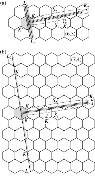
Figure 1: Cutting lines for (a) $(n,m)=(6,3)$, and (b) $(7,4)$ SWNTs. In each figure, shadow areas show three different choices of the 2D BZ of graphene. $S_{1}S_{2}$ short segments denote conventional cutting lines, while $L_{1}L_{2}$ long segment is another definition of 1D BZ. Here $d=3$, $d_{R}=3$, $T=\sqrt{21}a$, $|\mbox{\boldmath$C$}_{h}|=3\sqrt{7}a$ and $N=42$ for $(6,3)$ SWNT, and $d=1$, $d_{R}=3$, $T=\sqrt{31}a$, $|\mbox{\boldmath$C$}_{h}|=\sqrt{93}a$ and $N=62$ for $(7,4)$ SWNT.

Let us briefly review on the definition of the cutting lines for discussing their orbital angular momenta. There are arbitrary definitions for a complete set of the cutting lines as well as there are arbitrary definitions for 2D BZ of graphene as shown in Fig. 1. The detailed description on the definitions of the cutting lines is found in the review article. Samsonidze et al. (2003) Instead of the conventional definition of the cutting lines with short segments, Saito et al. (1998) the following definition of the cutting lines with long segments,

$$k\frac{\mbox{\boldmath$K$}_{2}}{|\mbox{\boldmath$K$}_{2}|}+\mu\mbox{\boldmath$K$}_{1},$$ (1)

with

$$-\frac{\pi}{T}\frac{N}{d}\leq k<\frac{\pi}{T}\frac{N}{d},~{}~{}\text{and}~{}~{}\mu=0,\cdots,d-1,$$ (2)

which is derived from the helical and rotational symmetries, White et al. (1993) is convenient to consider the properties under the $C_{d}$ rotational symmetry. [See the long segments $L_{1}L_{2}$ in Fig. 1 defined by Eqs. (1) and (2).] Here the separation of cutting lines $\mbox{\boldmath$K$}_{1}=(-t_{2}\mbox{\boldmath$b$}_{1}+t_{1}\mbox{\boldmath$b$}_{2})/N$ is perpendicular to the cutting lines and represents the discreteness of the wavevector in the circumference direction, and

$$\mbox{\boldmath$K$}_{2}=\frac{m\mbox{\boldmath$b$}_{1}-n\mbox{\boldmath$b$}_{2}}{N},$$ (3)

is the vector of short cutting lines in the conventional definition, Saito et al. (1998) where $\mbox{\boldmath$b$}_{1}=(2\pi/a)(1/\sqrt{3},1)$ and $\mbox{\boldmath$b$}_{2}=(2\pi/a)(1/\sqrt{3},-1)$ are the reciprocal lattice vectors of graphene, $t_{1}$ and $t_{2}$ are integers defined by $t_{1}=(2m+n)/d_{R}$, $t_{2}=-(2n+m)/d_{R}$. $T=a\sqrt{3(n^{2}+m^{2}+nm)}/d_{R}$ is the 1D nanotube lattice constant, $N=2(n^{2}+m^{2}+nm)/d_{R}$ is the number of A (B) atoms in the nanotube 1D unit cell, $a=2.46$Å is the lattice constant of graphene.

The rectangle defined by the two vectors $d\mbox{\boldmath$K$}_{1}$ and $N\mbox{\boldmath$K$}_{2}/d$ which surrounds the set of the longer cutting lines (see the vertically-long shadowed rectangle in Fig. 1) is equivalent to the 2D BZ of graphene. The corresponding unit vectors in the real space are the vector $\mbox{\boldmath$C$}_{h}/d$, and the vector given by $\mbox{\boldmath$R$}=p_{h}\mbox{\boldmath$a$}_{1}+q_{h}\mbox{\boldmath$a$}_{2}$ where $p_{h}$ and $q_{h}$ satisfy the relation of $mp_{h}-nq_{h}=d$. Jishi et al. (1993, 1994) The component of $R$ in the direction of nanotube axis is expressed by

$$a_{z}=\frac{Td}{N},$$ (4)

which corresponds to shortest distance between two A (B) atoms in the axis direction, because of the definition of $R$. Jishi et al. (1993, 1994) Note that the inversion of the range of $k/2\pi$ is equal to $a_{z}$. Because each cutting line defined by Eqs. (1) and (2) is equal to $N\mbox{\boldmath$K$}_{2}/d$, all independent $k$ states for the given angular momentum $\mu$ are represented in a single cutting line. Here, the orbital angular momentum of a state is defined by $\mu$ in Eq. (2).

It would be worthful to compare the present definition [Eq. ((2))] with conventional definition of the cutting lines, Saito et al. (1998) $-\pi/T\leq k<\pi/T$, and $\mu=0,\cdots,N-1$. [See the set of the short segments $S_{1}S_{2}$ in Fig. 1.] In the conventional definition, every $d$ cutting lines belongs to the same orbital angular momentum, that is, these cutting lines can mapped onto a single longer cutting line by translations with reciprocal lattice vectors. Therefore, the long cutting lines is convenient to consider the properties under the $C_{d}$ rotational symmetry since an orbital angular momentum and a cutting line are one-to-one correspondence.

Hereafter we focus on the m-SWNTs, in which there are cutting lines passing through the $K$ and $K^{\prime}$ points. As proven in the Appendix A (and shown in Figs. 1 (a) and (b) as examples), the long cutting line $L_{1}L_{2}$ of $\mu=0$ passes through both $K$ and $K^{\prime}$ points for the metal-2 nanotubes, whereas cutting line passes only through $K$ or $K^{\prime}$ points for the metal-1 nanotubes. The metal-2 nanotubes are further classified into metal-2$p$ and metal-2$m$ by the conditions, Saito et al. (2005)

$${\rm mod}\left(\frac{m}{d},3\right)=\left\{\begin{array}[]{cl}1&\text{~{}~{}for metal-2$p$},\\ 2&\text{~{}~{}for metal-2$m$}.\\ \end{array}\right.$$ (5)

It is also shown in the Appendix A [and in Fig. 1 (b) as an example] that the $K$ point is located at $1/6$ ($5/6$) position and the $K^{\prime}$ point is located at $5/6$ ($1/6$) position on the long cutting line of $\mu=0$ for metal-2$p$ (metal-2$m$) nanotubes. Note that the positions of the $K$ and $K^{\prime}$ points on the long 1D BZ are the opposite to these on the short 1D BZ. For the metal-1 nanotubes, the cutting lines of $\mu=\pm N/3$ ($\mu=\mp N/3$) pass through the $K$ and $K^{\prime}$, respectively, for $d_{X}=2$ ($d_{X}=1$) where $d_{X}={\rm mod}[(2n+m)/d,3)]$, as shown in the previous work for the conventional short cutting lines. Saito et al. (2005) Even though $\mu=\pm N/3$ may exceed the range $0\leq\mu\leq d-1$, the expression is convenient because the $K$ and $K^{\prime}$ points are mapped onto the center of the long cutting lines, which corresponds to 1D wavenumber of $k=0$. Other choices, e.g. $\mu={\rm mod}[(2n+m)/3,d]$ and $\mu={\rm mod}[(2m+n)/3,d]$ given in Ref.  Lunde et al., 2005, may map the $K$ and $K^{\prime}$ points away from the $\Gamma$ point of 1D BZ [see the longer cutting lines of $\mu=2$ and $\mu=1$ in Fig. 1 (a) for the $(n,m)=(6,3)$ metal-1 nanotube].

III Numerical Calculation

The two valleys $K$ and $K^{\prime}$ are decoupled for the finite-length metal-1 nanotubes with the $C_{d}$ rotational symmetry, since the two valleys belongs to states with different orbital angular momenta. For this case, energy levels show nearly fourfold degeneracy and its small lift by the spin-orbit interaction, as will be confirmed in numerical calculation in the Appendix §B.1. On the other hand, the two valleys can couple for the finite-length metal-2 nanotubes even both ends keep the $C_{d}$ rotational symmetry. Here we perform numerical calculation of finite-length SWNTs to investigate the valley coupling for the metal-2 nanotubes. Vernier-scale-like spectrum will be shown for an orthogonal-shaped boundary. Nearly fourfold degeneracy and its small lift, which is not due to the spin-orbit interaction for shorter nanotubes, will be shown for a so-called minimal boundary. Vernier-scale-like spectra for an armchair nanotube and a capped metal-2 nanotube will also be shown in the Appendix §B.2.

The numerical calculation is done using the extended tight-binding method, Samsonidze et al. (2004) in which $\pi$ and $\sigma$ orbitals at each carbon atom is considered, and the hopping and overlap integrals between the orbitals are evaluated from the ab initio calculation Porezag et al. (1995) for interatomic distances of up to 10 bohr. Since the systems we focus on are the finite-length nanotubes, the electronic states are calculated by solving the generalized eigenvalue problems with bases being from all orbitals in the systems. The optimized geometrical structure given by the previous energy band calculation Izumida et al. (2009) is utilized for determining the positions of carbon atoms. Three-dimensional structure is taken into account in the calculation, therefore the curvature effects Izumida et al. (2009, 2012) are automatically included. Spin degrees of freedom, and the atomic spin-orbit interaction $V_{\rm SO}=6$ meV on each carbon atom, Izumida et al. (2009) are also taken into account. A tiny magnetic field ($B=10^{-6}$ T, corresponding spin splitting is $\sim 10^{-8}$ meV) parallel to the nanotube axis is applied to separate the two degenerate states of the Kramers pairs in the calculation. The tube axis ($z$) is chosen as the spin quantization axis. In the following, two types of the boundaries are considered. The first type of the boundary has a geometry constructed simply cut by the plane orthogonal to the nanotube axis. Here we call this boundary orthogonal boundary. This boundary generally contains Klein-type terminations at which terminated site neighbors two empty sites Klein (1994) [see red site in Fig. 2 (a) for $(n,m)=(7,4)$]. The second type of the boundary has a geometry removing the Klein-terminations from the orthogonal boundary [see Fig. 3 (a) for $(n,m)=(7,4)$]. For both types, the edge has minimum number of empty sites [dashed circles in Figs. 2 (a) and 3 (a)]. Further, the number of empty sites are the same with that of dangling bonds for the second type. The second type of the boundary is called minimal boundary. Akhmerov and Beenakker (2008) In the numerical calculation, to eliminate the dangling bonds, each single dangling bond at the ends is terminated by a hydrogen atom, and the Klein-type termination is represented by two hydrogen atoms. Kusakabe and Maruyama (2003) Both boundaries keep the $C_{d}$ rotational symmetry of the SWNTs.

III.1 Vernier spectrum

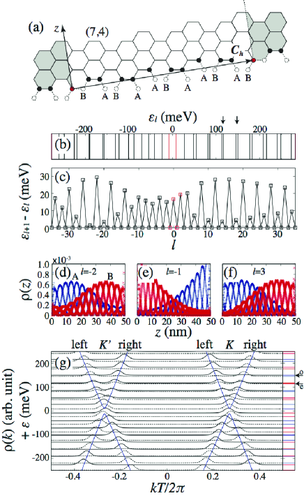
Figure 2: (Color online) Boundary shape, calculated energy levels and eigenstates for $(7,4)$ nanotube of $50.17$ nm length with the ends of orthogonal boundary. (a) Unfolded tube near the left end. The empty sites are represented by the dashed circles, and the carbon atoms at the boundary are marked by the solid circles. The red sites represent the Klein-type termination. The shadowed areas repeat the structure in the unshadowed area. (b) Energy levels $\varepsilon_{l}$ in $-35\leq l\leq 35$. $l$ is the energy level index numbered in ascending order of the energy and $l=0$ corresponds to the HOMO level. (c) Level separation, $\varepsilon_{l+1}-\varepsilon_{l}$, as a function of $l$. The levels of $-1\leq l\leq 2$ indicated by red color in (b) and (c) are slowly decaying modes. (d)-(f) Local density (d) $l=-2$, (e) $l=-1$ and (f) $l=3$. Blue shows that for A-sublattice, and red shows that for B-sublattice. (g) Zone-folded intensity plot of Fourier transform of wavefunction on A-sublattice for each level as a function of $k$. The energy for each level is added for each intensity plot. The intensities for states of spin-up-majority are shown. They are presented by either solid or dashed lines in turn in increasing the energy to show them clearly. The blue lines show the energy band calculated under the periodic boundary condition. Right figure in (g) shows the energy levels of the even parity (blue lines) and the odd parity (red lines) for $V_{\rm SO}=0$. The arrows with e (even) and o (odd) in (g) and in (b) show the states exhibiting intravalley coupling with the same parity. In (d)-(g), the components of orbital and spin are summed up for each site or each wavenumber.

Figure 2 (b) shows the calculated energy levels $\varepsilon_{l}$ near the charge neutral point for (7,4) nanotube of $50.17$ nm length with the orthogonal boundary for both ends. Here $l$ is the energy level index numbered in ascending order of the energy, and $l=0$ corresponds to the level of highest occupied molecular orbital (HOMO). To show the degeneracy behavior, the level separation, $\varepsilon_{l+1}-\varepsilon_{l}$, which corresponds to the addition energy in the tunneling spectroscopy measurements, Tarucha et al. (1996) is plotted in Fig. 2 (c). The levels of $-1\leq l\leq 2$ are slowly decaying modes that appear in the energy gap caused by the curvature of nanotube surface [the local densities of $l=-2$, $l=-1$ and $l=-3$ are shown in Figs. 2 (d)-(f) as examples]. The origin of the slowly decaying modes will be discussed in §IV. The level separation show oscillatory behavior between nearly fourfold [near $l\sim-25$ ($\varepsilon\sim-190$ meV) and $l\sim 13$ ($115$ meV)] and twofold [$l\sim-7$ ($\varepsilon\sim-55$ meV)] degeneracies. The behavior is understood by (i) the asymmetric velocities between left- and right-going waves in the same valley pointed out in the previous work, Izumida et al. (2012) and (ii) the strong intervalley coupling. The strong intervalley coupling is confirmed by the intensity plot in the wavenumber as shown in Fig. 2 (g). In this plot, the intensities for the states of spin-up-majority (with spin-up polarization more than $50\%$, in the calculation the polarization exceeds $99\%$) are shown. Note that the intensity at $k$ for the spin-up-majority and that at $-k$ for the spin-down-majority in spin degenerate levels are the same because of the time-reversal symmetry. For this case, the intensity plots for the spin-up-majority and that for the spin-down-majority almost coincides with each other for each of degenerate levels, that is, the orbital state of spin-up-majority and that of spin-down-majority are almost the same. Each eigenfunction shows the strong intensity only at the left-going wave at the $K$-valley ($K^{\prime}$-valley) and right-going wave at the $K^{\prime}$-valley ($K$-valley). The strong intervalley coupling combined with the asymmetric velocities causes the two types of the equal interval energy levels, $\hbar v_{\rm L}^{(K)}\pi/L_{\rm NT}$ and $\hbar v_{\rm R}^{(K)}\pi/L_{\rm NT}$, like the vernier scale. Izumida et al. (2012) The period of the two- to fourfold oscillation is not constant but has the energy dependence, for instance, the period becomes longer for the positive energy region. This is because the velocities has energy dependence reflecting the deviation from the linear energy band. The velocity difference between left- and right-going waves becomes smaller for the higher energy region in the conduction band. We can also see the intravalley coupling when the two levels are close to each other, for instance, $\varepsilon_{l}\sim$ 83 meV and 115 meV as shown by arrows in the left of Fig. 2 (g). The coupling occurs between the same parity states which will be discussed in §IV.

III.2 Valley degeneracy and lift of degeneracy

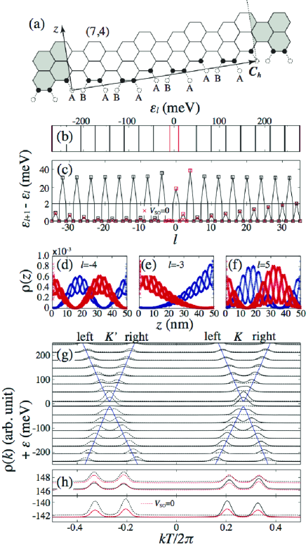
Figure 3: (Color online) Boundary shape, calculated energy levels and eigenstates for $(7,4)$ nanotube of $50.17$ nm length with the ends of minimal boundary. (a) Unfolded tube near the left end. (b) Energy levels $\varepsilon_{l}$ in $-35\leq l\leq 35$. (c) Level separation $\varepsilon_{l+1}-\varepsilon_{l}$ as a function of $l$. The case of absence of spin-orbit interaction is shown by the red cross in the lower panel. (d)-(f) Local density for (d) $l=-4$, (e) $l=-3$ and (f) $l=5$. (g) The zone-folded intensity plot of Fourier transform of wavefunction on A-sublattice for each level. The intensities for the states of spin-up-majority are shown. (h) Enlarged plot of (g) near $\varepsilon_{l}=147$ meV (upper panel) and $\varepsilon_{l}=-142$ meV (lower panel). The case of absence of spin-orbit interaction is shown by the red dashed lines.

Figure 3 (b) shows the calculated energy levels $\varepsilon_{l}$ for $50.17$ nm length (7,4) nanotube with the minimal boundary for both ends. The levels of $-3\leq l\leq 4$ indicated with red lines are the slowly decaying modes in the energy gap [the local density of $l=-3$ is shown in Fig. 3 (e) as an example]. Above and below the energy gap, the level separation shows almost equal interval reflecting the linear energy dispersion. Fig. 3 (c) shows that each of levels shows nearly fourfold degeneracy, which is very different from that in Fig. 2 (c). As shown in the lower panel of Fig. 3 (c), the degeneracy is lifted of the order of meV. The lift of the degeneracy is clearly observed even for the absence of the spin-orbit interaction in some energy region, for instance, $\varepsilon\mathrel{\mathchoice{\lower 2.58334pt\vbox{\halign{$\m@th\displaystyle\hfil#\hfil$\cr>\crcr\sim\crcr}}}{\lower 2.58334pt\vbox{\halign{$\m@th\textstyle\hfil#\hfil$\cr>\crcr\sim\crcr}}}{\lower 2.58334pt\vbox{\halign{$\m@th\scriptstyle\hfil#\hfil$\cr>\crcr\sim\crcr}}}{\lower 2.58334pt\vbox{\halign{$\m@th\scriptscriptstyle\hfil#\hfil$\cr>\crcr\sim\crcr}}}}100$ meV. From the intensity plot in the wavenumber in Fig. 3 (g), each level show almost equal intensity between the left- and right-going waves in the same valley, showing the valley degeneracy. The enlarged plot near $\varepsilon_{l}=147$ meV and $\varepsilon_{l}=-142$ meV in Fig. 3 (h) shows the effect of the spin-orbit interaction. The four levels near $\varepsilon_{l}=147$ meV show splitting into two spin-degenerate levels with $\Delta\varepsilon\sim 2$ meV when the spin-orbit interaction is absent. The splitting and the intensities does not change much when the spin-orbit interaction is turned on. The four levels near $\varepsilon_{l}=-142$ meV, on the other hand, show almost degeneracy when the spin-orbit interaction is absent. When the spin-orbit interaction is turned on, they splits into two spin-degenerate levels with the splitting $\Delta\varepsilon\sim 0.3$ meV. At the same time, the state of spin-up-majority in lower energy shows the intensity only at the $K$-valley ($kT/2\pi\sim 0.3$) whereas that in higher energy shows the intensity only at the $K^{\prime}$-valley ($kT/2\pi\sim-0.3$). The splitting is thus induced by both an intrinsic property of finite-length nanotubes with the minimal boundary and the spin-orbit interaction.

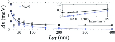
Figure 4: (Color online) Length dependence of splitting of fourfold degeneracy for $(7,4)$ nanotube with minimal boundary. Three same symbols at each length show the averaged splitting in the energy range $|\varepsilon_{l}|<250$ meV except the evanescent modes. The splittings are then also averaged for the three cases of the adjacent lengths, $L_{\rm NT}$, $L_{\rm NT}+a_{z}$, $L_{\rm NT}+2a_{z}$, because the splitting shows nearly three-fold oscillations with respect to the nanotube length in the unit of $a_{z}=0.022$ nm. Solid line shows the averaged splitting with the spin-orbit interaction, $V_{\rm SO}=6$ meV, dashed line shows that without the spin-orbit interaction. Inset shows the splitting as a function of the inverse of the length. The solid square with a bar (at $0.34$ meV) shows the absolute value of the spin-splitting averaged in the energy range $|\varepsilon_{l}|<250$ meV calculated from the energy band calculation.

Fig. 4 shows the splitting of the fourfold degeneracy for $(7,4)$ nanotube with minimal boundary as a function of nanotube length. The splitting is averaged in the energy range $|\varepsilon_{l}|<250$ meV except the evanescent modes. Further, because the splitting shows nearly three-fold oscillations with respect to the nanotube length in the unit of $a_{z}$, the average for the three cases is also taken. Without the spin-orbit interaction, the averaged splitting decreases when the length increases with $1/L_{\rm NT}$ dependence. For the actual case of the presence of spin-orbit interaction, the splitting for the longer nanotubes ($\mathrel{\mathchoice{\lower 2.58334pt\vbox{\halign{$\m@th\displaystyle\hfil#\hfil$\cr>\crcr\sim\crcr}}}{\lower 2.58334pt\vbox{\halign{$\m@th\textstyle\hfil#\hfil$\cr>\crcr\sim\crcr}}}{\lower 2.58334pt\vbox{\halign{$\m@th\scriptstyle\hfil#\hfil$\cr>\crcr\sim\crcr}}}{\lower 2.58334pt\vbox{\halign{$\m@th\scriptscriptstyle\hfil#\hfil$\cr>\crcr\sim\crcr}}}}200$ nm) are dominated by the spin-orbit interaction, as shown that the splitting is asymptotic to a constant value ($\sim 0.34$ meV).

IV Effective 1D model

The numerical calculation showed that the degeneracy of the energy levels, and the valley coupling in the eigenfunctions, are quite sensitive to the boundary shape. To investigate the microscopic mechanism of the valley coupling for given boundary conditions, we will introduce an effective 1D model, which extract the states near the two valleys remaining the atomic structure. This model can treat microscopic analysis of the coupling of two valleys, which can be an advantage from the conventional effective mass theory which treats each valley separately. It will be shown that the model shows evanescent and traveling nature of wavefunctions, and the comparison of the numbers of evanescent modes and the boundary conditions at the ends is an important key to understand the behaviors of valley coupling in the standing waves composed from the traveling modes. Analytical form of the discrete wavenumbers, the length dependence of the degeneracy lift, and the slowly decaying modes in the energy gap will also be shown.

IV.1 Effective 1D model

Let us consider the following nearest-neighbor tight-binding Hamiltonian,

$$H=\sum_{\vec{r}}\sum_{j=1}^{3}\gamma_{j}c_{{\rm A},\vec{r}}^{\dagger}c_{{\rm B},\vec{r}+\vec{\Delta}_{j}}+{\rm H.c.},$$ (6)

where $c_{{\rm A},\vec{r}}^{\dagger}$ is the creation operator of $\pi$ electron on A atom at site $\vec{r}$, and $c_{{\rm B},\vec{r}+\vec{\Delta}_{j}}$ is the annihilation operator of $\pi$ electron on the neighbor $j$-th B atom ($j=1,2,3$) at $\vec{r}+\vec{\Delta}_{j}$, $\vec{\Delta}_{j}$ is the vectors from A to nearest $j$-th B atoms (see $\vec{\Delta}_{j}$ in Fig. 11). The summation on $\vec{r}$ is taken over the finite-length SWNTs. $\gamma_{j}$ is the hopping integral between A and $j$-th B atom which is chosen as the real number, and, in general, they are different from one another because of the curvature of nanotube surface. For the simplicity, we ignore the spin degrees of freedom, the $\sigma$-orbitals, and the hopping to next nearest neighbor and further sites. The valley coupling in the standing waves can be discussed within this simplified model as shown later. The asymmetric velocities Izumida et al. (2012) and the spin-orbit interaction Izumida et al. (2009) are not able to be captured in this model, and they affect as the vernier-like spectrum and the spin-orbit splitting as shown in the numerical calculation in §III.

The construction of an effective 1D model is performed by projecting to an angular momentum $\mu$, as previously done for the achiral nanotubes. Balents and Fisher (1997) The effective 1D Hamiltonian for the metal-2 nanotubes is given by (see the Appendix C for the derivation),

$$H_{\mu=0}=\sum_{\ell}\sum_{j=1}^{3}\gamma_{j}a_{\ell}^{\dagger}b_{\ell+\Delta\ell_{j}}+{\rm H.c.},$$ (7)

where

$$\Delta\ell_{1}=t_{1}+t_{2},~{}~{}~{}~{}\Delta\ell_{2}=-t_{2},~{}~{}~{}~{}\Delta\ell_{3}=-t_{1},$$ (8)

and

$$a_{\ell}=\frac{1}{\sqrt{d}}\sum_{\vec{r}}c_{{\rm A},{\vec{r}}}\delta_{a_{z}\ell,z_{\vec{r}}},~{}~{}~{}~{}b_{\ell}=\frac{1}{\sqrt{d}}\sum_{\vec{r}}c_{{\rm B},{\vec{r}}}\delta_{a_{z}\ell,z_{\vec{r}}},$$ (9)

correspond to the $\mu=0$ Fourier components of the operators. The index $\ell$ is an integer specifying the 1D site. The summation is taken over for $d$ A atoms of $d$ B atoms which satisfy $z_{\vec{r}}=a_{z}\ell$ for $a_{\ell}$ and $b_{\ell}$, respectively. Note that there is a pair of A and B atoms on each $\ell$ because there are $d$ pairs of A and B atoms on the same $z$ for the metal-2 nanotubes. The model for $(n/d,m/d)=(7,4)$ SWNTs is depicted in Fig. 5. In Fig. 5, A_ℓ atom is connected to B_ℓ+6, B_ℓ-1, B_ℓ-5 atoms. Note that the Hamiltonian $H_{\mu=0}$ for $(7,4)$ SWNT is the total Hamiltonian since $d=1$. For this case the effective model has the same bond connection with the original model.

Figure 5: (Color online) Effective one-dimensional model for $(n/d,m/d)=(7,4)$ SWNTs in which $(t_{1},t_{2})=(5,-6)$. The solid lines show the hopping between atoms. The red lines denote the hopping from (and to) A atom at $\ell$-site.

IV.2 Modes of 1D model

Eigenfunctions of Eq. (7) are expressed as linear combinations of independent modes of the Hamiltonian. The modes of Eq. (7) are classified into traveling modes and evanescent modes. Coefficients of the traveling modes (and the evanescent modes) in each eigenfunction are determined by boundary conditions as will be discussed in the subsections below (§IV.3 - IV.5). Here we will show the independent modes of the Hamiltonian.

Hereafter we will consider the cases of $n\geq m>0$ for the metal-2 nanotubes, and then we have $|t_{2}|=-t_{2}>0$ and $t_{1}>0$. For an eigenstate $|\Phi\rangle=\sum_{\sigma\ell}\phi_{\sigma\ell}|\sigma\ell\rangle$ with energy $\varepsilon$ of the Hamiltonian (7), where $|\sigma\ell\rangle$ is the $\pi$-state at $\sigma$-atom ($\sigma={\rm A,B}$) on $\ell$-site, we have the following equations of motion,

$$\gamma_{1}\phi_{{\rm A}\ell+(|t_{2}|-t_{1})}+\gamma_{2}\phi_{{\rm A}\ell-|t_{2}|}+\gamma_{3}\phi_{{\rm A}\ell+t_{1}}=\varepsilon\phi_{{\rm B}\ell},$$ (10)

$$\gamma_{1}\phi_{{\rm B}\ell-(|t_{2}|-t_{1})}+\gamma_{2}\phi_{{\rm B}\ell+|t_{2}|}+\gamma_{3}\phi_{{\rm B}\ell-t_{1}}=\varepsilon\phi_{{\rm A}\ell}.$$ (11)

Substituting the following forms for the solutions,

$$\phi_{\sigma\ell+t}=\lambda^{t}\phi_{\sigma\ell},~{}~{}~{}~{}\phi_{{\rm B}\ell}=\eta\phi_{{\rm A}\ell},$$ (12)

for Eqs. (10) and (11), one gets the following simultaneous equations,

$$\gamma_{1}\lambda^{|t_{2}|-t_{1}}+\gamma_{2}\lambda^{-|t_{2}|}+\gamma_{3}\lambda^{t_{1}}=\varepsilon\eta,$$ (13)

$$\gamma_{1}\lambda^{-(|t_{2}|-t_{1})}+\gamma_{2}\lambda^{|t_{2}|}+\gamma_{3}\lambda^{-t_{1}}=\frac{\varepsilon}{\eta}.$$ (14)

Since $t_{1}+|t_{2}|=n/d+m/d$, there are $2(n/d+m/d)$ sets of solutions $(\lambda,\eta)$ for Eqs. (13) and (14) because each equation is the $(n/d+m/d)$-th order algebraic equation. For the case of $|\eta|<1$, we can call the mode A-like mode because the wavefunction is polarized at A atoms. On the other hand, we can call B-like mode for $|\eta|>1$. Further, we can call evanescent mode at left (right) side for $|\lambda|<1$ $(>1)$. The mode with $|\lambda|=|\eta|=1$ is called traveling mode. Let $\gamma$ be the average of $\gamma_{j}$, $\gamma=\sum\gamma_{j}/3$, and $\delta\gamma_{j}$ be the difference from the average, $\delta\gamma_{j}=\gamma_{j}-\gamma$. Because of the curvature of nanotube surface, $\delta\gamma_{j}\neq 0$. Hereafter we restrict our situation to consider the low energy states, $|\varepsilon/\gamma|\ll 1$, and small deviation of the hopping integrals from the average value, $|\delta\gamma_{j}/\gamma|\ll 1$. Hereafter of this subsection we will show main results for the total $2(n/d+m/d)$ modes. The detail derivation of the modes are given in Appendix D.

It is shown that there are $(n/d+m/d-2)$ A-like modes and $(n/d+m/d-2)$ B-like modes in the energy range considered. Further, by following Appendix B of Ref.  Akhmerov and Beenakker, 2008, the A-like modes are classified into $|t_{2}|-1$ evanescent modes at left side and $t_{1}-1$ evanescent modes at right side, whereas B-like modes are classified into $t_{1}-1$ evanescent modes at left side and $|t_{2}|-1$ evanescent modes at right side.

The remaining four modes are the traveling modes, or slowly decaying evanescent modes, depending on the energy. For the energy outside the energy gap induced by the curvature of nanotube surface, Hamada et al. (1992); Saito et al. (1992); Kane and Mele (1997); Ando (2000); Izumida et al. (2009) $|\varepsilon|>\varepsilon_{\rm gap}$, there are the following four traveling modes,

$$(\lambda,\eta)=\left(e^{{\rm i}k_{\ell}},e^{{\rm i}\Phi(k_{\ell})}\right),~{}~{}~{}~{}k_{\ell}=\tau^{\prime}k_{0}+k,$$ (15)

for the energies

$$\varepsilon=\pm|\gamma|\frac{\sqrt{3}a}{2a_{z}}\sqrt{k^{2}+k_{\rm I}^{2}}.$$ (16)

Here $k_{\ell}$ in Eq. (15) denotes four wavenumbers, where $\tau^{\prime}=\pm 1$ indicates the two valleys, and $k$, a wavenumber measured from $\tau^{\prime}k_{0}$, becomes either positive or negative, where $k_{0}=2\pi/3+k_{\rm R}$. [Note that $\tau=-\tau^{\prime}\beta$ corresponds to the index for the $K$ ($\tau=1$) or $K^{\prime}$ ($\tau=-1$) points, where $\beta=1$ ($\beta=-1$) is introduced for the metal-2$p$ (metal-2$m$) nanotubes.] $k_{\rm R}$ and $k_{\rm I}$ are the shift of the Dirac point in $\mbox{\boldmath$K$}_{2}$ and $\mbox{\boldmath$K$}_{1}$ direction, respectively, at the $\tau^{\prime}=1$ valley, because of the curvature of nanotube surface. From the previous energy band calculation with the extended tight-binding method, Izumida et al. (2009) they are evaluated to be

$$k_{\rm R}=-a_{z}\beta\zeta\frac{\sin 3\theta}{d_{t}^{2}},~{}~{}~{}~{}k_{\rm I}=a_{z}\beta^{\prime}\frac{\cos 3\theta}{d_{t}^{2}},$$ (17)

where $d_{t}=|\mbox{\boldmath$C$}_{h}|/\pi$ is the diameter of nanotube, $\theta=\arccos(2n+m)/2\sqrt{n^{2}+m^{2}+nm}$ is the chiral angle, and the coefficients are evaluated to be $\beta^{\prime}=0.0436$ nm and $\zeta=-0.185$ nm. The energy dispersion of Eq. (16) shows the energy gap

$$\varepsilon_{\rm gap}=|\gamma|\frac{\sqrt{3}a}{2a_{z}}|k_{\rm I}|.$$ (18)

The phase $\Phi$ in Eq. (15) is given by

$$\Phi(\tau^{\prime}k_{0}+k)=\tau^{\prime}\left(\frac{2\pi}{3}t_{2}+\beta\theta\right)+\arg\left[\frac{\gamma\left(k+{\rm i}k_{\rm I}\right)}{{\rm i}\varepsilon}\right].$$ (19)

Inside the gap, $|\varepsilon|<\varepsilon_{\rm gap}$, there are no traveling modes, but four slowly decaying evanescent modes, $(e^{i\tau^{\prime}k_{0}-\kappa},\eta)$, exist for the energies

$$\varepsilon=\pm|\gamma|\frac{\sqrt{3}a}{2a_{z}}\sqrt{k_{\rm I}^{2}-\kappa^{2}}.$$ (20)

Note that $\kappa$ can be either positive or negative. We have

$$|\eta|=\frac{|k_{\rm I}+\kappa|}{\sqrt{k_{\rm I}^{2}-\kappa^{2}}}.$$ (21)

For the case of $k_{\rm I}>0$, $|\eta|=\sqrt{\left(k_{\rm I}+\kappa\right)/\left(k_{\rm I}-\kappa\right)}$, then there are two B-like modes ($|\eta|>1$) which are slowly decaying near the left end ($\kappa>0$), and two A-like modes ($|\eta|<1$) which are slowly decaying modes near the right end ($\kappa<0$). The decay length is estimated to be $\sim 1/|k_{\rm I}|$, that could be much longer than that for the other $2(n/d+m/d-2)$ evanescent modes having the decay length of the order of carbon-carbon bond length. The slowly decaying modes appeared in the numerical calculation as shown in Fig. 2 (e) and Fig. 3 (e). Note that the appearance of slowly decaying modes for each sublattice depends on the sign of $k_{\rm I}$. Within the nearest-neighbor tight-binding model, the value might be estimated to be positive or negative with a small value depending on the application of the hopping parameters. Ando (2000) If $k_{\rm I}$ is estimated to be a negative value, the slowly decaying modes could appear by applying the Aharonov-Bohm (AB) flux. Sasaki et al. (2005, 2008); Margańska et al. (2011) We found that $k_{\rm I}$ is a positive value in the previous extended tight-binding calculation, Izumida et al. (2009) and the present numerical calculation showing the slowly decaying modes consistent with $k_{\rm I}>0$.

IV.3 Eigenfunctions of finite-length 1D model

An eigenstate of the finite-length 1D model is expressed by a linear combination of the modes derived in §IV.2. Let us extract only the traveling modes given in Eq. (15) in the eigenstate. Because of the real number of the hopping integrals in the Hamiltonian with $\mu=0$, the components of the traveling modes in the eigenstates are written by real functions of standing waves,

$$\phi_{{\rm A}\ell}=\sum_{r=\pm 1}c_{r}\cos\left[\left(k_{0}+k_{r}\right)\ell-\frac{\Phi(k_{0}+k_{r})}{2}+\theta_{r}\right],$$ (22)

$$\phi_{{\rm B}\ell}=\sum_{r=\pm 1}c_{r}\cos\left[\left(k_{0}+k_{r}\right)\ell+\frac{\Phi(k_{0}+k_{r})}{2}+\theta_{r}\right],$$ (23)

where $r=+1$ ($r=-1$) denotes the branch of right-going (left-going) wave at $k_{\ell}=k_{0}$. $k_{r}$ is the wavenumber of left-going or right-going waves measured from $k_{\ell}=k_{0}$. The cosine function for $r=+1$ ($r=-1$) is the linear combination of the right-going (left-going) wave at $k_{\ell}=k_{0}$ and its time-reversal state of the left-going (right-going) wave at $k_{\ell}=-k_{0}$. For the case that the left and right-going waves have the same velocity, the relation $k_{r=-1}=-k_{r=+1}$ holds in Eqs. (22) and (23) because the left- and right-going waves which compose $\phi_{{\rm A}\ell}$ and $\phi_{{\rm B}\ell}$ should have the same energy. For the asymmetric velocity case, Izumida et al. (2012) however, they are different from each other. We can choose that the coefficients to be positive, $c_{r}\geq 0$, and the phase $\theta_{r}$ to be real numbers. The coefficients, the phases, and the discretized wavenumbers $k_{r}$ are determined by applying boundary conditions at the left and the right ends.

It should be noted that the functions of Eqs. (22) and (23) themselves do not always describe the strong intervalley coupling, even though they have the functional form of linear combination of two valley states. For instance, when the two valleys are completely decoupled, each valley state as a linear combination of left- and right-going wave in the same valley is an eigenstate. Since the two valley states are degenerate, a linear combination of the two states, $c_{+1}=c_{-1}$ in Eqs. (22) and (23), is also an eigenstate of the Hamiltonian. When the spin-orbit interaction is introduced, the splitting of the doubly degenerate energy band occurs because of the lack of the inversion symmetry for the chiral nanotubes. Chico et al. (2004); Izumida et al. (2009) The valley degeneracy is lifted by the spin-orbit interaction, and the $K$-valley state with spin-up (spin-down) function and the $K^{\prime}$-valley state with spin-down (spin-up) function are the set of eigenfunctions for each Kramers pairs, as shown in the negative energy region in Figs. 3 (g) and (h). For this case, Eqs. (22) and (23) do not describe the orbital states for each spin state. However, for cases that the spin-orbit interaction is irrelevant such as Fig. 2 and $\varepsilon_{l}\mathrel{\mathchoice{\lower 2.58334pt\vbox{\halign{$\m@th\displaystyle\hfil#\hfil$\cr>\crcr\sim\crcr}}}{\lower 2.58334pt\vbox{\halign{$\m@th\textstyle\hfil#\hfil$\cr>\crcr\sim\crcr}}}{\lower 2.58334pt\vbox{\halign{$\m@th\scriptstyle\hfil#\hfil$\cr>\crcr\sim\crcr}}}{\lower 2.58334pt\vbox{\halign{$\m@th\scriptscriptstyle\hfil#\hfil$\cr>\crcr\sim\crcr}}}}100$ meV region in Fig. 3, Eqs. (22) and (23) could express the approximated orbital parts of the eigenstates in the finite-length metal-2 nanotubes.

IV.4 Parity symmetry

In order to discuss the boundary conditions, let us consider the parity symmetry of the 1D model, that is, the Hamiltonian is invariance by exchanging $a_{\ell}\leftrightarrow b_{N_{s}+1-\ell}$, where $N_{s}$ is the site index at the right end. This corresponds to an inversion symmetry of 1D lattice of Fig. 5. Using the parity symmetry, it is enough to consider only one of the two ends instead of both ends for the boundary conditions. We have the following relation on the wavefunctions,

$$\phi_{{\rm A}\ell}=p\phi_{{\rm B}N_{s}+1-\ell}~{}~{}\text{for any}~{}\ell,$$ (24)

where $p=\pm 1$ are the parity eigenvalues. Applying Eq. (24) to the standing waves in Eqs. (22) and (23), it is shown that one of the following three conditions should be satisfied,

$$\left\{\begin{array}[]{l}c_{+1}=0,\\ \exp\left({\rm i}\left[\left(k_{0}+k_{-1}\right)\left(N_{s}+1\right)+2\theta_{-1}\right]\right)=p,\\ \end{array}\right.$$ (25)

or

$$\left\{\begin{array}[]{l}c_{-1}=0,\\ \exp\left({\rm i}\left[\left(k_{0}+k_{+1}\right)\left(N_{s}+1\right)+2\theta_{+1}\right]\right)=p,\\ \end{array}\right.$$ (26)

or

$$\left\{\begin{array}[]{l}c_{r}\neq 0,\\ \exp\left({\rm i}\left[\left(k_{0}+k_{r}\right)\left(N_{s}+1\right)+2\theta_{r}\right]\right)=p,\\ \end{array}\right.$$ (29)

$$\text{for both }r=\pm 1.$$

The selection from Eqs. (25) - (29) depends on the boundary type, as is discussed below. Note that the parity symmetry of the 1D model corresponds to the $C_{2}$ rotational symmetry around the $C_{2}$ axis at center of a carbon-carbon bond in the direction perpendicular to the nanotube axis in the original SWNT. Barros et al. (2006) This is not an inversion symmetry of the original SWNT. Unlike the inversion operation, the $C_{2}$ rotation change the spin-direction. The parity symmetry for the eigenfunctions is broken in the presence of the spin-orbit interaction since the orbital state and the spin state are coupled. This is the reason why the parity states for the absence of the spin-orbit interaction are shown in Fig. 2 (g).

IV.5 Boundary conditions

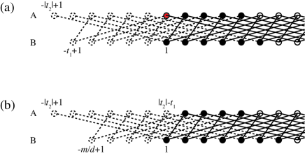
Figure 6: (Color online) Two examples of the left end classified into (a) orthogonal boundary condition in which $|t_{2}|$ A sites and $t_{1}$ B sites are empty, and (b) minimal boundary condition in which $n/d$ A sites and $m/d$ B sites are empty, for $(n/d,m/d)=(7,4)$ nanotubes. The dashed circles represent the empty atomic sites and the dashed lines represent the missing bonds. The solid circles represent the carbon atoms at the boundary, and the red circle represents the Klein-type termination.

There is a variety on the geometry of the boundary shape. Here we explicitly consider two types of boundary, one gives strong valley coupling and another gives decoupling of two valleys. For a moment we exclude the armchair nanotubes which are classified into metal-2 nanotubes. The first type of the boundary is depicted in Fig. 6 (a). At the left end, both A and B atoms are terminated at the same $z$ coordinate (at $\ell=1$). The end is constructed by cutting nanotube orthogonal to the axis direction. This is the orthogonal boundary. Each A atom in $1\leq\ell\leq|t_{2}|-t_{1}$ connects to a B atom, corresponds to the Klein-type termination. Klein (1994) Each A atom in $|t_{2}|-t_{1}+1\leq\ell\leq t_{1}$ connects to two B atoms, and each B atom in $1\leq\ell\leq|t_{2}|$ connects to two A atoms. For this case, the following boundary conditions are imposed,

$$\phi_{{\rm A}\ell}=0~{}~{}\text{at}~{}~{}\ell=-|t_{2}|+1,\cdots,0.$$ (30)

$$\phi_{{\rm B}\ell}=0~{}~{}\text{at}~{}~{}\ell=-t_{1}+1,\cdots,0.$$ (31)

The number of boundary conditions for $\phi_{{\rm A}\ell}$ is $|t_{2}|$, and that for $\phi_{{\rm B}\ell}$ is $t_{1}$. As shown in §IV.2, in the low energy region, there are totally $|t_{2}|+1$ relevant modes (two traveling and $|t_{2}|-1$ evanescent modes) for $\phi_{{\rm A}\ell}$, and $t_{1}+1$ relevant modes for $\phi_{{\rm B}\ell}$ at the left end. Therefore, the wavefunctions for A- and B-sublattices can be determined with an arbitrarity of the amplitude. In addition, as shown in the Appendix E, the wavefunctions of A- and B-sublattices share a common coefficient for this case. Therefore, we have two solutions for the wavefunctions of Eqs. (22) and (23): $c_{+1}=0$ and $\theta_{-1}$ is determined, or, $c_{-1}=0$ and $\theta_{+1}$ is determined. The coefficient of $c_{+1}=0$ or $c_{-1}=0$ reflects only the intervalley scattering at the ends. For this case, either Eq. (25) or Eq. (26) should be satisfied. Therefore, we get the following discretization for the wavenumbers,

$$k_{r}=\frac{l_{p}\pi}{N_{s}+1}+\delta k_{r},$$ (32)

where $l_{p}$ is an even (odd) integer for $p=1$ ($p=-1$), $\delta k_{r}=(2L\pi-2\theta_{r})/(N_{s}+1)-k_{0}$ is a small offset, an integer $L$ may be chosen as $L=[2\theta_{r}+k_{0}(N_{s}+1)]/2\pi$, where $[x]$ is Gauss’s symbol representing the greatest integer that is less than or equal to $x$. In general, $\delta k_{r=+1}\neq\delta k_{r=-1}$, therefore the energy levels are not degenerate between $r=+1$ and $r=-1$. The corresponding expression is used in the previous articles Rubio et al. (1999); Yaguchi and Ando (2001); Mayrhofer and Grifoni (2006, 2007); del Valle et al. (2011) for the armchair nanotubes. Eq. (32) simply shows the discretization for the standing waves of $r=1$ and $r=-1$. The discrete energy levels have generally twofold degeneracy reflecting the spin degrees of freedom. When we consider the asymmetric velocities, Izumida et al. (2012) vernier-scale-like discrete energy levels are obtained as shown in Fig. 2. Note that the integer $L$, then the offset $\delta k$ shows nearly three-fold oscillations when the nanotube length $N_{s}$ changes because $L\simeq[(N_{s}+1)/3]$ for $k_{0}\simeq 2\pi/3$. Energy levels for finite-length of $N_{s}$ and $N_{s}+3$ are almost identical while that of $N_{s}+1$ and $N_{s}+2$ are generally different one another, which is confirm in our numerical calculation (not shown). Because the analysis above relies on the low energy condition, deviation such as the intravalley coupling in the same parity state as shown in Fig. 2 could occur for a larger energy region.

The second type of the boundary is depicted in Fig. 6 (b). Each A atom in $|t_{2}|-t_{1}+1\leq\ell\leq t_{1}$ connects to two B atoms in the body, and each B atom in $1\leq\ell\leq|t_{2}|$ connects to two A atoms in the body. This boundary is the minimal boundary in Fig. 3. The following conditions are imposed for the wavefunctions,

$$\phi_{{\rm A}\ell}=0~{}~{}\text{at}~{}~{}\ell=-|t_{2}|+1,\cdots,|t_{2}|-t_{1}.$$ (33)

$$\phi_{{\rm B}\ell}=0~{}~{}\text{at}~{}~{}\ell=-m/d+1,\cdots,0.$$ (34)

The number of conditions for $\phi_{{\rm A}\ell}$ is $n/d$, and that for $\phi_{{\rm B}\ell}$ is $m/d$. Akhmerov and Beenakker (2008) Because the number of boundary conditions for $\phi_{{\rm A}\ell}$ is larger than or equal to the number of relevant modes of A-sublattice at the left end, $n/d\geq|t_{2}|+1$, the standing wave for A-sublattice should be zero at the left end, which corresponds to “fixed boundary condition” for the standing waves. Then we get the condition $c_{-1}=c_{+1}$ so that the envelope function of the A-sublattice becomes zero at the left end. This condition, $c_{-1}=c_{+1}$, reflects that only the intravalley scattering occurs at the ends. We also have that the phase difference $\theta_{+1}-\theta_{-1}$ is fixed to be $\pi/2$ in the linear dispersion region in which the relation $\Phi(k_{0}-k)=\Phi(k_{0}+k)+\pi$ holds. Therefore, the wavefunction of A-sublattice vanishes at the left end because of the envelope function $\sin(k\ell)$. For this case, Eq. (29) should be satisfied for both $r=1$ and $r=-1$. We have the following discretized wavenumbers,

$$\frac{k_{+1}-k_{-1}}{2}=\frac{l\pi+\theta_{+1}-\theta_{-1}}{N_{s}+1},$$ (35)

for both parity states $p=\pm 1$, where $l$ is an integer. Note that the left hand side of Eq. (35) is $k$ if $k=k_{+1}=-k_{-1}$ holds for the case of symmetric Dirac cone in which the energy is given by Eq. (16). The corresponding expression is shown for the zigzag nanotubes. Rocha et al. (2002); del Valle et al. (2011) For a given $l$, the two parity states has the same wavenumber. Therefore the two states have the same energy. In larger energy region, we may have a parity dependent deviation for the phase difference from $\pi/2$ such as $\theta_{+1}-\theta_{-1}=\pi/2-\vartheta_{p}k$, where $-\vartheta_{p}k$ represents the deviation from $\pi/2$ and $\vartheta_{p}$ is a coefficient of the deviation. For this case we have $k=(l+1/2)\pi/(N_{s}+1+\vartheta_{p})$, then there are the parity splitting for the degenerate energy levels,

$$\Delta\varepsilon=\left|\gamma\right|\frac{\sqrt{3}a}{2a_{z}}k\frac{\delta\vartheta}{N_{s}},$$ (36)

where $\delta\vartheta=\vartheta_{p=1}-\vartheta_{p-1}$. The dependence of the inverse of the length on the energy splitting is consistent with the numerical calculation in Fig. 4.

For the armchair nanotubes, the orthogonal and the minimal boundary conditions are identical. (Note that $n/d=m/d=t_{1}=|t_{2}|=1$ for the armchair nanotubes.) Both for $\phi_{{\rm A}\ell}$ and $\phi_{{\rm B}\ell}$, the number of boundary conditions is one and there are two relevant modes. Therefore the same discussion with the orthogonal boundary condition is available.

IV.6 Slowly decaying modes

Finally we comment on the number of slowly decaying modes in the calculation. For a SWNT which is longer than the slowly decaying modes, the modes appear at the zero energy. As shown in §IV.2, the number of B-like evanescent modes, including the two slowly decaying modes, at the left end is $t_{1}+1$ for the metal-2 nanotubes with $\mu=0$ states. For the orthogonal boundary, the number of boundary conditions for the B-sublattice at the left end is $t_{1}$ Therefore, the number of independent evanescent modes is $t_{1}+1-t_{1}=1$ for each spin and each end. There are total 4 independent evanescent modes for both ends orthogonal boundary. Since the longest evanescent mode dominates in each eigenstate, 4 slowly decaying modes appear.

For the minimal boundary, the number of boundary conditions for the B-sublattice at the left end is $m/d$, then the number of the independent evanescent modes is $t_{1}+1-m/d=(n-m)/3d+1$ for each spin and each end. Since the number of slowly decaying modes is two in the independent evanescent modes, 8 slowly decaying modes appear for both ends minimal boundary, as shown in Fig. 3. The remaining independent evanescent modes with shorter decay length would also appear for the case of $(n-m)/3d+1\geq 3$.

For the SWNTs shorter than the decay length of the slowly decaying modes, the slowly decaying modes appear at finite energies to satisfy the boundary conditions, as shown in Figs. 2 and 3. Note that the A-like evanescent modes do not appear at the left end because the number of A-like evanescent modes, $|t_{2}|-1$, is smaller than that of the boundary conditions for the above boundaries, $|t_{2}|$ or $n/d$.

V Conclusion

In summary, we studied the discrete energy levels in the finite-length m-SWNTs. For the metal-1 nanotubes with the $C_{d}$ rotational symmetry, the two valleys are decoupled in the eigenfunctions because they have different orbital angular momenta. The energy levels have nearly fourfold degeneracy and the spin-orbit interaction lifts the degeneracy in the order of meV. For the metal-2 nanotubes, on the other hand, the two valley states have the same orbital angular momentum and they are strongly coupled for the orthogonal boundary and the cap-termination as well as the armchair nanotubes. The energy levels showed the vernier-like spectrum reflecting the asymmetric velocities and the strong valley coupling. For the metal-2 nanotubes with minimal boundary, nearly fourfold behavior was observed, reflecting nearly decoupling of two valleys. For this case, the parity splitting overcomes the spin-orbit splitting for the short nanotubes. The effective one-dimensional model explained the coupling of the two valleys, appearance of the slowly decaying modes caused by the curvature-induced shift of the Dirac point, the length dependence of the parity splitting. The spectrum types for nanotube types discussed in this paper are summarized in Table 1.

Table 1: Summary of the degeneracy for the finite-length m-SWNTs with $C_{d}$ rotational symmetry around the tube axis, and with $C_{2}$ rotational symmetry around the axis perpendicular to the tube axis. Metal-1 nanotubes satisfy the relation $d_{R}=d$, and metal-2 nanotubes satisfy the relation $d_{R}=3d$. OB means the orthogonal boundary, MB means the minimal boundary, and SO means spin-orbit. The armchair nanotubes with armchair edges are categorized in Metal-2 (OB). Chirality dependence of the spin-orbit splitting for each valley is given in Ref.  Izumida et al., 2009.

Type	Spectrum
Metal-1	nearly fourfold, SO splitting
Metal-2 (OB)	vernier-scale-like
Metal-2 (MB)	nearly fourfold, SO splitting, parity splitting

In this paper we restrict the finite-length SWNTs without any external field. The finite-length effects studied in this paper will directly checked in devices made of all nano-carbons including SWNTs. In the many experimental setup with the metal-gated SWNTs, additional potentials could be created to confine the electrons inside the tubes. However, the nanotube ends may still influence to the electrons in a center region because of the Klein tunneling through the barriers Steele et al. (2009) or for the nanotubes on the metal electrodes. Nygård et al. (1999) Furthermore we did not consider effects of Coulomb interaction between electrons, which can be the same order of the level spacing of the single-particle energy. One of the main feature could be captured within the so-called constant interaction model, Sapmaz et al. (2005) which simply increase the label-independent constant term in the addition energy. The degeneracy behavior studied in this paper could be useful for understanding the orbital-related correlated electrons such as the Kondo effect Liang et al. (2002); Jarillo-Herrero et al. (2005b); Makarovski et al. (2007); Cleuziou et al. (2013) and the Pauli blockade. Pei et al. (2012) The interaction could also cause intervalley scattering as well as intravalley scattering, and might affects especially on the valley decoupling features. The effective 1D model derived in this paper could be a lattice model to treat the Coulomb interaction for the given geometry of the chirality with the boundary for the recent observed 1D correlated electron effects such as the Mott insulator Deshpande et al. (2009) and the Wigner crystallization. Deshpande and Bockrath (2008); Pecker et al. (2013) The effects of additional potential effects as well as the Coulomb interaction in the finite-length SWNTs with boundaries should be clarified in future study.

Appendix A Long cutting lines passing through $K$ and $K^{\prime}$ points for metal-1 and metal-2 nanotubes

Here, we will show the fact that a long cutting line passes through both $K$ and $K^{\prime}$ points for the metal-2 nanotubes, whereas cutting line passes only through $K$ or $K^{\prime}$ points for the metal-1 nanotubes.

If a cutting line passes through both $K$ and $K^{\prime}$ points, the cutting line should also passes through a $\Gamma$ point because the $K^{\prime}$ point sits on the opposite side of $K$ point with respect to the $\Gamma$ point. Therefore, the cutting line should be $\mu=0$. If the $\mu=0$ cutting line does not pass a $K$ point, there is no cutting line which passes both $K$ and $K^{\prime}$ points for a given $(n,m)$.

The condition that the $\mu=0$ cutting line passes through a $K$ point is expressed by,

$$\left(\alpha+\frac{1}{3}\beta\right)\mbox{\boldmath$K$}_{2}=\overrightarrow{\Gamma K}+j_{1}\mbox{\boldmath$b$}_{1}+j_{2}\mbox{\boldmath$b$}_{2},$$ (37)

where $\overrightarrow{\Gamma K}=(2\mbox{\boldmath$b$}_{1}+\mbox{\boldmath$b$}_{2})/3$ is the vector from $\Gamma$ point to $K$ point in a hexagonal BZ, $\alpha$, $\beta$, $j_{1}$ and $j_{2}$ are integers. Here $\beta$ is introduced as follows;

$$\beta=\left\{\begin{array}[]{cl}0&\text{~{}~{}for metal-1},\\ +1&\text{~{}~{}for metal-2$p$},\\ -1&\text{~{}~{}for metal-2$m$}.\\ \end{array}\right.$$ (38)

In Eq. (37), we used the already known fact that a $K$ point is mapped onto the center of a short cutting line for the metal-1 nanotubes, whereas it is mapped onto 5/6 (1/6) position of a short cutting line for the metal-2$p$ metal-2$m$ nanotubes. Saito et al. (2005) It should be noted that the following relation holds for the metal-2 nanotubes,

$${\rm mod}\left(\frac{n}{d},3\right)={\rm mod}\left(\frac{m}{d},3\right),$$ (39)

because of the relation $(n-m)/3d=[(2n+m)-(2m+n)]/d_{R}=-t_{1}-t_{2}$. In order to satisfy Eq. (37), $j_{1}$, $j_{2}$ and $\alpha$ should satisfy the following equations. By comparing the coefficients of $\mbox{\boldmath$b$}_{1}$ and $\mbox{\boldmath$b$}_{2}$ in Eq. (37), we have,

$$j_{1}n+j_{2}m=-\frac{1}{3}\left(2n+m\right),$$ (40)

$$\alpha=\left(\frac{2}{3}+j_{1}\right)\frac{N}{m}-\frac{\beta}{3}.$$ (41)

For the case of metal-2 nanotubes, it will be shown that the following $j_{1}$ and $j_{2}$ satisfy the conditions Eqs. (40) and (41),

$$j_{1}=-\frac{1}{3}\left(\beta\frac{m}{d}+2\right),$$ (42)

$$j_{2}=-\frac{1}{3}\left(-\beta\frac{n}{d}+1\right).$$ (43)

Note that the right hand sides of Eqs. (42) and (43) are integers because of Eqs. (5) and (39) for the metal-2 nanotubes. By substituting Eq. (42) for Eq. (41), $\alpha$ is given by

$$\alpha=-\frac{\beta}{3}\left(\frac{N}{d}+1\right).$$ (44)

Because $N=2(n^{2}+m^{2}+nm)/d_{R}=[(2m+n)(2n+m)-3nm]/d_{R}$ and $d_{R}=3d$ for the metal-2 nanotubes, the following relation folds,

$$\frac{N}{d}=-3t_{1}t_{2}-\frac{nm}{d^{2}}.$$ (45)

Using this, Eq. (44) becomes

$$\alpha=\beta t_{1}t_{2}+\frac{\beta}{3}\left(\frac{nm}{d^{2}}-1\right).$$ (46)

The right hand side of Eq. (46) is an integer because of the relation ${\rm mod}(nm/d^{2},3)=1$, which can be derived from Eqs. (5) and (39). Therefore, Eq. (37) is satisfied by the set of integers of Eqs. (42), (43) and (46) for the metal-2 nanotubes. From the left hand side of Eq. (37) and Eq. (44), it is shown that the $K$ point is located at $1/6$ ($5/6$) position of the longer cutting line defined by Eqs. (1) and (2) with $\mu=0$ for the metal-2$p$ (metal-2$m$) nanotubes.

For the case of metal-1 nanotubes, dividing Eq. (40) by $d$, one gets,

$$j_{1}\frac{n}{d}+j_{2}\frac{m}{d}=\frac{1}{3}t_{2}.$$ (47)

Because $t_{2}$ is not a multiple of 3 for the metal-1 nanotubes, any integers of $j_{1}$ and $j_{2}$ cannot satisfy Eq. (47). Therefore, there is no cutting line passing through both $K$ and $K^{\prime}$ points for the metal-1 nanotubes.

Appendix B Numerical calculation for metal-1, armchair and capped metal-2 nanotubes

Here we will show some numerical calculation of the finite-length metal-1, armchair, and capped metal-2 nanotubes using the extended tight-binding model. As expected, the metal-1 with $C_{d}$ rotational symmetry will exhibit nearly fourfold degeneracy and its lift by the spin-orbit interaction. On the other hand, the armchair and the capped metal-2 nanotubes will exhibit the vernier-like spectra as well as Fig. 2.

B.1 Energy levels for metal-1 nanotubes

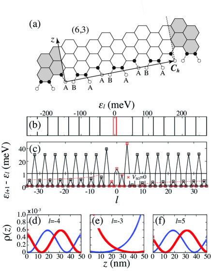
Figure 7: (Color online) Boundary shape, calculated energy levels and eigenstates for $(6,3)$ nanotube of $50.15$ nm length with both ends minimal boundary as shown in (a). (b) Energy levels $\varepsilon_{l}$ in $-35\leq l\leq 35$. (c) Level separation, $\varepsilon_{l+1}-\varepsilon_{l}$, as a function of $l$. The dashed lines in the lower panel show the spin-orbit splitting for corresponding energy calculated by the energy band calculation. (d)-(f) Local density for (c) $l=-4$, (d) $l=-3$ and (e) $l=5$.

Figure 7 (b) shows the energy levels for (6,3) nanotube with $50.15$ nm length with the minimal boundary for both ends keeping $C_{3}$ ($d=3$) rotational symmetry. The left end is depicted in Fig. 7 (a). There are the slowly decaying modes ($-3\leq l\leq 4$) in the energy gap between $\varepsilon_{l=-4}=-44$ meV and $\varepsilon_{l=5}=53$ meV. Above and below the energy gap, the level separation shows almost equal interval reflecting the quantization of the linear energy dispersion. Fig. 7 (c) shows that each levels show nearly fourfold degeneracy. The levels show complete fourfold degeneracy for the case of absence of spin-orbit interaction. The spin-orbit interaction lifts the fourfold degeneracy as expected in the energy band calculation. Izumida et al. (2009) Other metal-1 nanotubes, for instance, metallic (9,0)-zigzag nanotubes, also show similar behaviors with Fig. 7, nearly fourfold degeneracy and lift of the degeneracy by the spin-orbit interaction (not shown). In addition, finite length (9,0) nanotubes show the edge states decaying in the length scale of carbon-carbon bond, not on but below the charge neutral point, as the effect of the next nearest-neighbor hopping process. Sasaki et al. (2006)

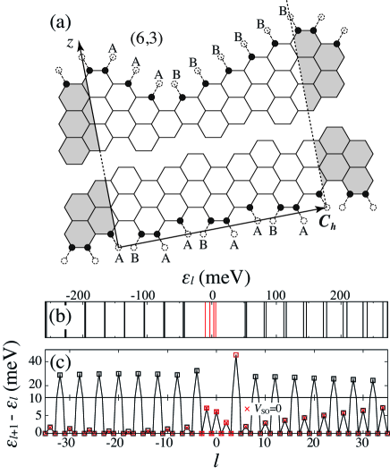
Figure 8: (Color online) Boundary shape and calculated energy levels $\varepsilon_{l}$ for $(6,3)$ nanotube of $50.63$ nm length. (a) Unfolded tube near the left (lower) and right (upper) ends. The upper end is cut along the $n\mbox{\boldmath$a$}_{1}$ and $m\mbox{\boldmath$a$}_{2}$. Note that both ends are classified into the minimal boundary. (b) Energy levels $\varepsilon_{l}$ in $-35\leq l\leq 35$. (c) Level separation, $\varepsilon_{l+1}-\varepsilon_{l}$, as a function of $l$.

When the rotational symmetry at the end is broken, the valley degeneracy and its lift by the spin-orbit interaction will not be clearly observed. Figure 8 shows the energy level for (6,3) nanotube with $50.63$ nm length, in which the one side of the end is cut along the $n\mbox{\boldmath$a$}_{1}$ and $m\mbox{\boldmath$a$}_{2}$ and the other side is the same with Fig. 7. The system loses the $C_{3}$ rotational symmetry which is possessed in the case of Fig. 7. The large lift of the fourfold degeneracy, for instance, $\Delta\epsilon\mathrel{\mathchoice{\lower 2.58334pt\vbox{\halign{$\m@th\displaystyle\hfil#\hfil$\cr>\crcr\sim\crcr}}}{\lower 2.58334pt\vbox{\halign{$\m@th\textstyle\hfil#\hfil$\cr>\crcr\sim\crcr}}}{\lower 2.58334pt\vbox{\halign{$\m@th\scriptstyle\hfil#\hfil$\cr>\crcr\sim\crcr}}}{\lower 2.58334pt\vbox{\halign{$\m@th\scriptscriptstyle\hfil#\hfil$\cr>\crcr\sim\crcr}}}}$ 6 meV in $\varepsilon\mathrel{\mathchoice{\lower 2.58334pt\vbox{\halign{$\m@th\displaystyle\hfil#\hfil$\cr>\crcr\sim\crcr}}}{\lower 2.58334pt\vbox{\halign{$\m@th\textstyle\hfil#\hfil$\cr>\crcr\sim\crcr}}}{\lower 2.58334pt\vbox{\halign{$\m@th\scriptstyle\hfil#\hfil$\cr>\crcr\sim\crcr}}}{\lower 2.58334pt\vbox{\halign{$\m@th\scriptscriptstyle\hfil#\hfil$\cr>\crcr\sim\crcr}}}}200$ meV, is not caused by the spin-orbit interaction, but due to the mixing of the two valley degrees of freedom by breaking of the rotational symmetry.

In the end of this subsection, we comment on valley mixing effect by the spin-orbit interaction. Strictly speaking, the spin-orbit interaction could mix the states in two valleys because spin-up states in $\mu=1$ cutting line, which passes the $K^{\prime}$ point, and spin-down states in $\mu=2$ cutting line, which passes the $K$ point, have the same total angular momentum, $3/2$ (see Fig. 1 (a) for the cutting lines). Mixing of the two valleys may give an additional effect from the spin-orbit splitting, such as the parity splitting in Fig. 3 or the splitting in Fig. 8 for the absence of $C_{3}$ rotational symmetry. Such valley mixing effects, however, seem to be irrelevant in Fig. 7, which simply shows the splitting as expected from the band calculation.

B.2 Vernier spectra for (6,6)-armchair and capped (7,4) nanotubes

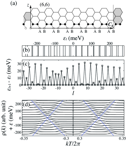
Figure 9: (Color online) Boundary shape, calculated energy levels and intensity plot in wavenumber for $(6,6)$ armchair nanotube of $50.05$ nm length. (a) Unfolded tube near the left end. (b) Energy levels in $\varepsilon_{l=-35}\leq\varepsilon\leq\varepsilon_{l=35}$. (b) Level separation, $\varepsilon_{l+1}-\varepsilon_{l}$, as a function of $l$. (c) Intensity plot of Fourier transform of wavefunction on A-sublattice for each level. The intensities for the states of spin-up-majority are shown. The blue lines show the energy band calculation under the periodic boundary condition.

Figure 9 shows the energy levels for (6,6)-armchair nanotube with $50.05$ nm length. The energy levels show the similar behaviors with the vernier-like spectrum in Fig. 2. This can be understood by (i) the strong intervalley coupling and (ii) the asymmetric velocities, as well as Fig. 2. For the armchair nanotubes, it can be shown using the effective 1D model that even channel from $(a_{\ell}+b_{\ell})/\sqrt{2}$ states and odd channel from $(a_{\ell}-b_{\ell})/\sqrt{2}$ states are decoupled each other for this boundary, and the even (odd) channel has the energy band with left-going states at the $K$-valley ($K^{\prime}$-valley) and right-going states at the $K^{\prime}$-valley ($K$-valley). Therefore, no intravalley mixing is seen in Fig. 9 (c). The period of the two- to fourfold oscillation is not constant but has the energy dependence, for instance, the period becomes longer for the positive energy region. This is because the velocities has energy dependence reflecting the deviation from the linear energy band. The velocity difference between left- and right-going waves becomes smaller for the higher energy region in the conduction band as well as the (7,4) nanotube.

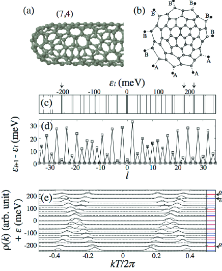
Figure 10: (Color online) Boundary shape, calculated energy levels and intensity plot in wavenumber for $(7,4)$ nanotube of $49.56$ nm length with both-ends-capped. (a) 3D and (b) 2D representation of the cap structure. In (b), the solid circles indicate the A and B atoms connected to the cap region, and the open circle indicate the carbon atoms in the cap region at the left end. (c) Energy levels $\varepsilon_{l}$ in $-35\leq l\leq 35$. (d) Level separation $\varepsilon_{l+1}-\varepsilon_{l}$ as a function of $l$. (e) Intensity plot of Fourier transform of wavefunction on A-sublattice for each level. Right figure in (e) shows the energy levels of the even parity (blue lines) and the odd parity (red lines) for $V_{\rm SO}=0$. The arrows in (c) and (e) show the states exhibiting intravalley coupling.

We show another case exhibiting the vernier-like spectrum for a capped nanotube, which would be more abundant than the orthogonal boundary containing the Klein-terminations. Figure 10 shows the calculated energy levels for both-side-capped (7,4) nanotubes of $49.56$ nm length. In the calculation, the cap structure is formed by using the graph theory, Brinkmann et al. (2002, 2010) in which the cap region is defined outside the end cut along the $n\mbox{\boldmath$a$}_{1}$ and $m\mbox{\boldmath$a$}_{2}$. There are two cap obeying the isolated pentagon rule for (7,4) nanotube, one has 55 and the other has 57 carbon atoms at the cap region. The cap with 57 carbon atoms is used in the calculation. To connect the cap and the body smoothly, the structure is optimized by the molecular mechanics method with the Universal force field (UFF) in the Gaussian program. Frisch et al. Even the optimization method gives less accuracy on the electronic fine structure such as the curvature-induced energy gap and the spin-orbit interaction, we could discuss the intervalley coupling in the eigenfunctions from the semi-quantitative calculation. The vernier-like spectrum is seen in the calculated energy levels. As shown in the plot of Fourier transform, in general, each level is formed from a left-going wave of one valley and a right-going wave of another valley, that corresponds to $|c_{r}/c_{-r}|\ll 1$ ($r=1$ or $-1$) in Eqs. (22) and (23) reflecting the strong intervalley coupling. For closer two levels, the intravalley mixing between the same parity states is also seen, for instance, $\varepsilon_{l}\sim-208$ meV, $181$ and $213$ meV. The vernier-like spectrum similar with Fig. 10 is also obtained for another cap obeying the isolated pentagon rule with 55 carbon atoms in the numerical calculation (not shown).

The strong valley coupling for the case of cap-termination may be understood in the 1D model as follows. The boundary conditions at the left end can be given by $\phi_{{\rm A}\ell}=\phi_{{\rm c}\ell_{\rm c}}$ for $n$ sets of $(\ell_{\rm A},\ell_{\rm c})$ and $\phi_{{\rm B}\ell}=\phi_{{\rm c}\ell_{\rm c}}$ for $m$ sets of $(\ell_{\rm A},\ell_{\rm c})$, where $\ell_{\rm A}$ ($\ell_{\rm B}$) is the index of the coordinate of A-sublattice (B-sublattice) and $\ell_{\rm c}$ is that of cap. For the amplitudes $\phi_{{\rm c}\ell_{\rm c}}$, there are $N_{\rm c}$ equations of motion. In general, $\phi_{{\rm c}\ell_{\rm c}}$ shows oscillation in the length scale of carbon-carbon bond. Therefore, one also expects the fast oscillations for the wavefunctions of A- and B-sublattices, which can be formed under the strong intervalley coupling of $|c_{r}/c_{-r}|\ll 1$ for $r=1$ or $-1$.

Appendix C Derivation of effective 1D Model

Here we will show the detailed of the derivation of the effective 1D model given in §IV.1.

In the cylindrical coordinate system in which the tube axis coincides the $z$ axis, the components of $\vec{\Delta}_{j}$ appearing in Eq. (6) ($\vec{\Delta}_{j}$ is depicted in Fig. 11) is given by

$$\Delta\theta_{1}=\pi\frac{n+m}{n^{2}+m^{2}+nm},$$ (48)

$$\Delta\theta_{2}=-\pi\frac{m}{n^{2}+m^{2}+nm},$$ (49)

$$\Delta\theta_{3}=-\pi\frac{n}{n^{2}+m^{2}+nm},$$ (50)

and

$$\Delta z_{1}=-a_{z}\frac{n-m}{3d},$$ (51)

$$\Delta z_{2}=a_{z}\frac{2n+m}{3d},$$ (52)

$$\Delta z_{3}=-a_{z}\frac{2m+n}{3d}.$$ (53)

Let us consider the following Fourier transform in the circumference direction for the operators,

$$c_{\sigma(\mu,z)}=\frac{1}{\sqrt{d}}\sum_{\vec{r}}{\rm e}^{-{\rm i}\mu\theta_{\vec{r}}}c_{\sigma{\vec{r}}}\delta_{z,z_{\vec{r}}},$$ (54)

where $\sigma={\rm A,B}$, and $z=a_{z}\ell$ denotes the lattice position of A atoms on the nanotube axis, $\ell$ is the integer for the lattice position. The summation on $\vec{r}$ is taken place for a given $z$. The inverse Fourier transform is given by

$$c_{\sigma{\vec{r}}}=\frac{1}{\sqrt{d}}\sum_{\mu=0}^{d-1}{\rm e}^{{\rm i}\mu\theta_{\vec{r}}}c_{\sigma(\mu,z_{\vec{r}})}.$$ (55)

Substituting Eq. (55) for the Hamiltonian Eq. (6), the Hamiltonian can be decomposed into projected Hamiltonian for $\mu$-th angular momentum $H_{\mu}$,

$$H=\sum_{\mu}H_{\mu},$$ (56)

$$H_{\mu}=\sum_{z}\sum_{j=1}^{3}\gamma_{j}{\rm e}^{{\rm i}\mu\Delta\theta_{j}}c_{{\rm A}(\mu,z)}^{\dagger}c_{{\rm B}(\mu,z+\Delta z_{j})}+{\rm H.c.},$$ (57)

By selecting the $\mu$ values in which $H_{\mu}$ contains states near the Fermi energy, one gets an effective 1D Hamiltonian.

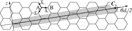
Figure 11: Coordinates for $(7,4)$ nanotube. The dashed lines show the interval of the 1D lattice constant $a_{z}=Td/N$. For this case, $d=1$, $T=\sqrt{31}a$ and $N=62$ .

Because of our main interest, let us focus on the metal-2 nanotubes. For the metal-2 nanotubes, $\Delta z_{j}$ can be expressed by

$$\Delta z_{1}=a_{z}(t_{1}+t_{2}),$$ (58)

$$\Delta z_{2}=-a_{z}t_{2},$$ (59)

$$\Delta z_{3}=-a_{z}t_{1}.$$ (60)

It should be mentioned that there is a B atom at $\beta\mbox{\boldmath$C$}_{h}/d_{R}$ from each A atom, that is, there are $d$ pairs of A and B atoms on the same $z$ for the metal-2 nanotubes. [For example, see Fig. 11 for the coordinates of $(n,m)=(7,4)$ metal-2$p$ nanotube ($d=1$).] We consider only $H_{\mu=0}$ and use the simplified notation,

$$c_{{\rm A}(\mu=0,z=a_{z}\ell)}\rightarrow a_{\ell},~{}~{}~{}~{}c_{{\rm B}(\mu=0,z=a_{z}\ell)}\rightarrow b_{\ell}.$$ (61)

and $\Delta\ell_{j}=\Delta z_{j}/a_{z}$, then we get Eq. (7) for the effective 1D Hamiltonian for the metal-2 nanotubes.

Appendix D Mode analysis of effective 1D model

Here we will discuss the detail derivation of the modes of Eqs. (13) and (14).

As a general property, when $(\lambda,\eta)$ is a set of solution of Eqs. (13) and (14), $(1/\lambda,1/\eta)$ is another set of solution since the equations are equivalent by changing $(\lambda,\eta)\leftrightarrow(1/\lambda,1/\eta)$. For a solution $(\lambda,\eta)$, the complex conjugates, $(\lambda^{*},\eta^{*})$ is also another set of solution since $\gamma_{j}$ and $\varepsilon$ are real numbers.

We will start from the traveling modes ($|\lambda|=|\eta|=1$) in the solutions of Eqs. (13) and (14). For the traveling modes, Eqs. (13) and (14) are equivalent as mutual complex conjugate. Let us first consider the flat graphene case, $\delta\gamma_{j}=0$. By noting the fact that the left hand side of Eq. (13) is zero for $\lambda=e^{\pm{\rm i}2\pi/3}$ because of the relations Eqs. (5) and (39), we can expand at the wavenumbers $k_{\ell}=\pm 2\pi/3$ which correspond to the two Dirac points. It is shown that there are four traveling modes for a given energy; $(\lambda,\eta)=\left(e^{{\rm i}k_{\ell}},e^{{\rm i}\Phi(k_{\ell})}\right)$, where $k_{\ell}=\tau^{\prime}2\pi/3+k^{\prime}$ denotes four wavenumbers for a given energy. We restricted in the linear dispersion regime, in which the energy and $k^{\prime}$ has the relation,

$$\varepsilon=\pm|\gamma|\frac{\sqrt{3}a}{2a_{z}}|k^{\prime}|.$$ (62)

The phase in Eq. (15) is given by

$$\Phi\left(\tau^{\prime}\frac{2\pi}{3}+k^{\prime}\right)=\tau^{\prime}\left(\frac{2\pi}{3}t_{2}+\beta\theta\right)+\arg\left(\frac{\gamma k^{\prime}}{{\rm i}\varepsilon}\right),$$ (63)

$\beta=\pm 1$ is the value defined in Eq. (38) for the metal-2 nanotubes, and $\theta$ is the chiral angle. Because of the time-reversal symmetry, we have $\Phi(k_{\ell})=-\Phi(-k_{\ell})$.

When $\delta\gamma_{j}\neq 0$, the above analysis should be modified as follows. For a state with wavenumber $k_{\ell}=\tau^{\prime}2\pi/3+k^{\prime}$, by considering the contribution of lowest order of $k^{\prime}$ and $\delta\gamma_{j}/\gamma$, Eq. (13) is written as,

$$-{\rm i}\gamma e^{\tau^{\prime}{\rm i}\left(\frac{2\pi}{3}t_{2}+\beta\theta\right)}\frac{\sqrt{3}a}{2a_{z}}\left[\left(k^{\prime}-\tau^{\prime}k_{\rm R}\right)+{\rm i}k_{\rm I}\right]=\varepsilon\eta.$$ (64)

Here $k_{\rm R}$ and $k_{\rm I}$ satisfy the following relations,

$$k_{\rm R} =\frac{2a_{z}}{\sqrt{3}a}\beta\sum_{j=1}^{3}\frac{\delta\gamma_{j}}{\gamma}\sin\left[\theta+\frac{2\pi}{3}\left(j-2\right)\right],$$ (65)

$$k_{\rm I} =\frac{2a_{z}}{\sqrt{3}a}\sum_{j=1}^{3}\frac{\delta\gamma_{j}}{\gamma}\cos\left[\theta+\frac{2\pi}{3}\left(j-2\right)\right].$$ (66)

$k_{\rm R}$ and $k_{\rm I}$ relate to the shift of the Dirac point in $\mbox{\boldmath$K$}_{1}$ and $\mbox{\boldmath$K$}_{2}$ direction, respectively, from the $K$ or $K^{\prime}$ points in 2D BZ because of the curvature of nanotube surface. By comparing with the energy band calculation with the extended tight-binding method, Izumida et al. (2009) they have the relations in Eq. (17). From Eq. (64), it is shown that there are the following four traveling modes,

$$(\lambda,\eta)=\left(e^{{\rm i}k_{\ell}},e^{{\rm i}\Phi(k_{\ell})}\right),~{}~{}~{}~{}k_{\ell}=\tau^{\prime}k_{0}+k,$$ (67)

for the energy outside the energy gap, $|\varepsilon|>\varepsilon_{\rm gap}$, where the energy gap

$$\varepsilon_{\rm gap}=|\gamma|\frac{\sqrt{3}a}{2a_{z}}|k_{\rm I}|$$ (68)

is induced by the curvature of nanotube surface. Kane and Mele (1997); Ando (2000); Izumida et al. (2009) After Eq. (67), $k$ is the wavenumber measured from $\tau^{\prime}k_{0}=\tau^{\prime}\left(2\pi/3+k_{\rm R}\right)$, which is the bottom (top) position of the conduction (valence) band. The energy and $k$ has the following relation

$$\varepsilon=\pm|\gamma|\frac{\sqrt{3}a}{2a_{z}}\sqrt{k^{2}+k_{\rm I}^{2}},$$ (69)

and the phase is given by

$$\Phi(\tau^{\prime}k_{0}+k)=\tau^{\prime}\left(\frac{2\pi}{3}t_{2}+\beta\theta\right)+\arg\left[\frac{\gamma\left(k+{\rm i}k_{\rm I}\right)}{{\rm i}\varepsilon}\right].$$ (70)

Inside the gap, $|\varepsilon|<\varepsilon_{\rm gap}$, there are no traveling modes, but four slowly decaying evanescent modes exist. Near the band edges, the modes can be analyzed by changing $\left(k^{\prime}-\tau^{\prime}k_{\rm R}\right)\rightarrow i\kappa$ in Eq. (64) and in a pair equation derived from (14). Then it is shown straightforwardly that the modes $(e^{i\tau^{\prime}k_{0}-\kappa},\eta)$ have the energy

$$\varepsilon=\pm|\gamma|\frac{\sqrt{3}a}{2a_{z}}\sqrt{k_{\rm I}^{2}-\kappa^{2}}.$$ (71)

Note that $\kappa$ can be either positive or negative. From Eqs. (64) and (71), we have

$$|\eta|=\frac{|k_{\rm I}+\kappa|}{\sqrt{k_{\rm I}^{2}-\kappa^{2}}}.$$ (72)

The remaining $2(n/d+m/d)-4$ modes can be classified into $(n/d+m/d-2)$ A-like modes and $(n/d+m/d-2)$ B-like modes. For the A-like modes, using $|\varepsilon/\gamma|\ll 1$, $|\delta\gamma_{j}/\gamma|\ll 1$ and $|\eta|<1$, Eqs. (13) and (14) can be simplified as

$$\lambda^{n/d+m/d}+\lambda^{n/d}+1=0,$$ (73)

$$\eta=\frac{\varepsilon}{\gamma}\frac{1}{\lambda^{-(|t_{2}|-t_{1})}+\lambda^{|t_{2}|}+\lambda^{-t_{1}}}.$$ (74)

The first equation (73) has the roots $\lambda=e^{\pm{\rm i}2\pi/3}$ and the properties for these modes have already been captured as the traveling modes or the slowly decaying modes in the previous paragraphs. For the remaining $(n/d+m/d-2)$ solutions, the analysis given by Akhmerov and Beenakker Akhmerov and Beenakker (2008) is applicable. Note that Eq. (73) for $\lambda^{\prime}=\lambda^{n/d+m/d}$ is the same with Eq. (3.7a) in Ref.  Akhmerov and Beenakker, 2008. By following Appendix B of Ref.  Akhmerov and Beenakker, 2008, it is shown that there are $|t_{2}|-1$ roots which satisfy $|\lambda|<1$ (evanescent modes at the left side), and $t_{1}-1$ roots which satisfy $|\lambda|>1$ (evanescent modes at the right side) for Eq. (73). The second equation (74) determines $\eta$ for each $\lambda$. The similar discussion can be done for the B-like modes with the equations which are given by changing $n\leftrightarrow m$ (then $t_{1}\leftrightarrow|t_{2}|$) and $\eta\rightarrow 1/\eta$ in Eqs. (73) and (74). Then it is shown that there are $t_{1}-1$ modes which satisfy $|\lambda|<1$, and there are $|t_{2}|-1$ modes which satisfy $|\lambda|>1$ for the B-like modes.

Appendix E Traveling modes for A- and B-sublattices for a given boundary

Here we will show that one of the following relations should be hold for the orthogonal boundary: $c_{+1}=0$ and $\theta_{-1}$ is determined, or, $c_{-1}=0$ and $\theta_{+1}$ determined in Eqs. (22) and (23).

Let us first show a useful relation. The left hand side of Eq. (13) is rewritten as

$$\frac{1}{\lambda^{|t_{2}|}}\prod_{\tau^{\prime}=\pm}\left(\lambda-\lambda_{\tau^{\prime}}\right)\prod_{m_{1}=1}^{t_{2}-1}\left(\lambda-\lambda_{m_{1}}^{<}\right)\prod_{m_{2}=1}^{|t_{1}|-1}\left(\lambda-\lambda_{m_{2}}^{>}\right),$$

$$= \frac{1}{\lambda}\prod_{\tau^{\prime}=\pm}\left(\lambda-\lambda_{\tau^{\prime}}\right)\prod_{m_{1}=1}^{t_{2}-1}\left(-\lambda_{m_{1}}^{<}\right)$$

$$\times\prod_{m_{1}=1}^{t_{2}-1}\left(\frac{1}{\lambda}-\frac{1}{\lambda_{m_{1}}^{<}}\right)\prod_{m_{2}=1}^{|t_{1}|-1}\left(\lambda-\lambda_{m_{2}}^{>}\right),$$ (75)

where $\lambda_{\tau^{\prime}}=e^{{\rm i}\tau^{\prime}k_{0}}$, $\lambda_{m_{1}}^{<}$, and $\lambda_{m_{2}}^{>}$ are the roots of the left hand side, and we have $|\lambda_{m_{1}}^{<}|<1$, $|\lambda_{m_{2}}^{>}|>1$. In Eq. (75), it is shown that the value $\prod_{m_{1}=1}^{t_{2}-1}\left(-\lambda_{m_{1}}^{<}\right)$ is a real number because there is another root of $\lambda_{m_{1}}^{<*}$ for a complex root $\lambda_{m_{1}}^{<}$. For a traveling mode of $\lambda$ which has almost the same wavenumber with $k_{0}$ or $-k_{0}$, $\lambda^{-1}\prod_{\tau^{\prime}=\pm}\left(\lambda-\lambda_{\tau^{\prime}}\right)$ is a small real number. Let us explicitly consider a traveling mode close to $\lambda_{+}$, $(\lambda_{+},e^{{\rm i}\Phi})$. From Eqs. (13) and (75), we have the following relation, which will be used later,

$$\prod_{m_{1}=1}^{t_{2}-1}\left(\frac{1}{\lambda_{+}}-\frac{1}{\lambda_{m_{1}}^{<}}\right)\prod_{m_{2}=1}^{|t_{1}|-1}\left(\lambda_{+}-\lambda_{m_{2}}^{>}\right)=Re^{{\rm i}\Phi},$$ (76)

where $R$ is a finite real number.

For the limit of $|\varepsilon/\gamma|\ll 1$, the equations of motion for A- and B-sublattice are decoupled [see Eqs. (10) and (11)]. For this case, the wavefunctions of A- and B-sublattices under a boundary are determined separately, in general. We will show that, for the orthogonal boundary, the wavefunctions of A- and B-sublattices share a common coefficient for the traveling modes. The wavefunctions near the left end are written as the linear combination of the relevant modes as follows:

$$\phi_{{\rm A}\ell}=\sum_{\tau^{\prime}=\pm}c_{{\rm A}\tau^{\prime}}e^{-\tau^{\prime}{\rm i}\frac{\Phi}{2}}\lambda_{\tau^{\prime}}^{\ell}+\sum_{m_{1}=1}^{|t_{2}|-1}c_{{\rm A}m_{1}}\lambda_{m_{1}}^{<\ell},$$ (77)

$$\phi_{{\rm B}\ell}=\sum_{\tau^{\prime}=\pm}c_{{\rm B}\tau^{\prime}}e^{\tau^{\prime}{\rm i}\frac{\Phi}{2}}\lambda_{\tau^{\prime}}^{\ell}+\sum_{m_{2}=1}^{t_{1}-1}c_{{\rm B}m_{2}}\frac{1}{\lambda_{m_{2}}^{>\ell}}.$$ (78)

Note that there are two traveling modes for each sublattice in the limit of $|\varepsilon/\gamma|\ll 1$. The factors $e^{\mp\tau^{\prime}{\rm i}\frac{\Phi}{2}}$ are attached for the convenience of the discussion. Here we used that each evanescent mode of B-sublattice at the left end has a pair with that of A-sublattice at the right end, that is, for each pair of roots, the relation $\lambda_{\rm A}=1/\lambda_{\rm B}$ holds where $\lambda_{\rm A}$ is a root of Eq. (13) and $\lambda_{\rm B}$ is the corresponding root of Eq. (14). The coefficients are determined by employing boundary conditions. If $c_{{\rm A}\tau^{\prime}}=c_{{\rm B}\tau^{\prime}}$ is satisfied for both $\tau^{\prime}=\pm 1$, one of the following relations should be hold in Eqs. (22) and (23): $c_{+1}=0$ and $\theta_{-1}$ is determined, or, $c_{-1}=0$ and $\theta_{+1}$ is determined.

Let us consider the orthogonal boundary expressed in Eqs. (30) and (31). If $c_{{\rm A}\tau^{\prime}}=c_{{\rm B}\tau^{\prime}}$ is satisfied for both $\tau^{\prime}=\pm 1$ for this boundary, the following determinant should be zero.

$$D=\left|\begin{array}[]{cccccccc}e^{-{\rm i}\frac{\Phi}{2}}&e^{{\rm i}\frac{\Phi}{2}}&1&\cdots&1&0&\cdots&0\\ e^{-{\rm i}\frac{\Phi}{2}}\lambda_{+}^{-1}&e^{{\rm i}\frac{\Phi}{2}}\lambda_{-}^{-1}&\left(\lambda_{1}^{<}\right)^{-1}&\cdots&\left(\lambda_{|t_{2}|-1}^{<}\right)^{-1}&0&\cdots&0\\ \vdots&\vdots&\vdots&\ddots&\vdots&\vdots&\ddots&\vdots\\ e^{-{\rm i}\frac{\Phi}{2}}\lambda_{+}^{-|t_{2}|+1}&e^{{\rm i}\frac{\Phi}{2}}\lambda_{-}^{-|t_{2}|+1}&\left(\lambda_{1}^{<}\right)^{-|t_{2}|+1}&\cdots&\left(\lambda_{|t_{2}|-1}^{<}\right)^{-|t_{2}|+1}&0&\cdots&0\\ e^{{\rm i}\frac{\Phi}{2}}&e^{-{\rm i}\frac{\Phi}{2}}&0&\cdots&0&1&\cdots&1\\ e^{{\rm i}\frac{\Phi}{2}}\lambda_{+}^{-1}&e^{-{\rm i}\frac{\Phi}{2}}\lambda_{-}^{-1}&0&\cdots&0&\left(\frac{1}{\lambda_{1}^{>}}\right)^{-1}&\cdots&\left(\frac{1}{\lambda_{t_{1}-1}^{>}}\right)^{-1}\\ \vdots&\vdots&\vdots&\ddots&\vdots&\vdots&\ddots&\vdots\\ e^{{\rm i}\frac{\Phi}{2}}\lambda_{+}^{-t_{1}+1}&e^{-{\rm i}\frac{\Phi}{2}}\lambda_{-}^{-t_{1}+1}&0&\cdots&0&\left(\frac{1}{\lambda_{1}^{>}}\right)^{-t_{1}+1}&\cdots&\left(\frac{1}{\lambda_{t_{1}-1}^{>}}\right)^{-t_{1}+1}\\ \end{array}\right|.$$ (79)

By cofactor expansion and use the relation on the Vandermonde matrix, one gets the following relation,

$$D=\left(-1\right)^{\frac{t_{1}(t_{1}-1)}{2}+\frac{|t_{2}|(|t_{2}|-1)}{2}}\prod_{1\leq m_{1}<m_{2}\leq|t_{2}|-1}\left(\frac{1}{\lambda_{m_{1}}^{<}}-\frac{1}{\lambda_{m_{2}}^{<}}\right)\prod_{1\leq m_{1}<m_{2}\leq t_{1}-1}\left(\lambda_{m_{1}}^{>}-\lambda_{m_{2}}^{>}\right)$$

$$\times\left\{e^{{\rm i}\Phi}\prod_{m_{1}=1}^{t_{2}-1}\left(\frac{1}{\lambda_{-}}-\frac{1}{\lambda_{m_{1}}^{<}}\right)\prod_{m_{2}=1}^{|t_{1}|-1}\left(\lambda_{-}-\lambda_{m_{2}}^{>}\right)-e^{-{\rm i}\Phi}\prod_{m_{1}=1}^{t_{2}-1}\left(\frac{1}{\lambda_{+}}-\frac{1}{\lambda_{m_{1}}^{<}}\right)\prod_{m_{2}=1}^{|t_{1}|-1}\left(\lambda_{+}-\lambda_{m_{2}}^{>}\right)\right\}.$$ (80)

By using Eq. (76) in the second line of Eq. (80), one gets $D=0$. Therefore, one of the the following two relations should be held for the orthogonal boundary; $c_{+1}=0$ and $\theta_{-1}$ is determined, or, $c_{-1}=0$ and $\theta_{+1}$ is determined.

References

- Venema et al. (1999) L. C. Venema, J. W. G. Wildöer, J. W. Janssen, S. J. Tans, H. L. J. T. Tuinstra, L. P. Kouwenhoven, and C. Dekker, Science 283, 52 (1999).
- Lemay et al. (2001) S. G. Lemay, J. W. Janssen, M. van den Hout, M. Mooij, M. J. Bronikowski, P. A. Willis, R. E. Smalley, L. P. Kouwenhoven, and C. Dekker, Nature 412, 617 (2001).
- Liang et al. (2002) W. Liang, M. Bockrath, and H. Park, Phys. Rev. Lett. 88, 126801 (2002).
- Cobden and Nygård (2002) D. H. Cobden and J. Nygård, Phys. Rev. Lett. 89, 046803 (2002).
- Jarillo-Herrero et al. (2005a) P. Jarillo-Herrero, J. Kong, H. S. J. van der Zant, C. Dekker, L. P. Kouwenhoven, and S. De Franceschi, Phys. Rev. Lett. 94, 156802 (2005a).
- Moriyama et al. (2005) S. Moriyama, T. Fuse, M. Suzuki, Y. Aoyagi, and K. Ishibashi, Phys. Rev. Lett. 94, 186806 (2005).
- Sapmaz et al. (2005) S. Sapmaz, P. Jarillo-Herrero, J. Kong, C. Dekker, L. P. Kouwenhoven, and H. S. J. van der Zant, Phys. Rev. B 71, 153402 (2005).
- Maki et al. (2005) H. Maki, Y. Ishiwata, M. Suzuki, and K. Ishibashi, Jpn. J. Appl. Phys. 44, 4269 (2005).
- Cao et al. (2005) J. Cao, Q. Wang, and H. Dai, Nat. Mater. 4, 745 (2005).
- Makarovski et al. (2006) A. Makarovski, L. An, J. Liu, and G. Finkelstein, Phys. Rev. B 74, 155431 (2006).
- Moriyama et al. (2007) S. Moriyama, T. Fuse, and K. Ishibashi, Phys. Stat. Sol. B 244, 2371 (2007).
- Holm et al. (2008) J. V. Holm, H. I. Jørgensen, K. Grove-Rasmussen, J. Paaske, K. Flensberg, and P. E. Lindelof, Phys. Rev. B 77, 161406 (2008).
- Kuemmeth et al. (2008) F. Kuemmeth, S. Ilani, D. C. Ralph, and P. L. McEuen, Nature 452, 448 (2008).
- Jhang et al. (2010) S. H. Jhang, M. Marganska, Y. Skourski, D. Preusche, B. Witkamp, M. Grifoni, H. van der Zant, J. Wosnitza, and C. Strunk, Phys. Rev. B 82, 041404(R) (2010).
- Jespersen et al. (2011) T. S. Jespersen, K. Grove-Rasmussen, J. Paaske, K. Muraki, T. Fujisawa, J. Nygård, and K. Flensberg, Nat. Phys. 7, 348 (2011).
- Steele et al. (2013) G. A. Steele, F. Pei, E. A. Laird, J. M. Jol, H. B. Meerwaldt, and L. P. Kouwenhoven, Nat. Commun. 4, 1573 (2013).
- Ando (2000) T. Ando, J. Phys. Soc. Jpn. 69, 1757 (2000).
- Chico et al. (2004) L. Chico, M. P. Lopez-Sancho, and M. C. Munoz, Phys. Rev. Lett. 93, 176402 (2004).
- Huertas-Hernando et al. (2006) D. Huertas-Hernando, F. Guinea, and A. Brataas, Phys. Rev. B 74, 155426 (2006).
- Chico et al. (2009) L. Chico, M. P. López-Sancho, and M. C. Muñoz, Phys. Rev. B 79, 235423 (2009).
- Izumida et al. (2009) W. Izumida, K. Sato, and R. Saito, J. Phys. Soc. Jpn. 78, 074707 (2009).
- Jeong and Lee (2009) J.-S. Jeong and H.-W. Lee, Phys. Rev. B 80, 075409 (2009).
- Izumida et al. (2012) W. Izumida, A. Vikström, and R. Saito, Phys. Rev. B 85, 165430 (2012).
- Rubio et al. (1999) A. Rubio, D. Sánchez-Portal, E. Artacho, P. Ordejón, and J. M. Soler, Phys. Rev. Lett. 82, 3520 (1999).
- Yaguchi and Ando (2001) T. Yaguchi and T. Ando, J. Phys. Soc. Jpn. 70, 1327 (2001).
- Bulusheva et al. (1998) L. G. Bulusheva, A. V. Okotrub, D. A. Romanov, and D. Tomanek, J. Phys. Chem. A 102, 975 (1998).
- Rocha et al. (2002) C. G. Rocha, T. G. Dargam, and A. Latgé, Phys. Rev. B 65, 165431 (2002).
- McCann and Fal’ko (2004) E. McCann and V. I. Fal’ko, J. Phys.: Condens. Matter 16, 2371 (2004).
- Brey and Fertig (2006) L. Brey and H. A. Fertig, Phys. Rev. B 73, 235411 (2006).
- Akhmerov and Beenakker (2008) A. R. Akhmerov and C. W. J. Beenakker, Phys. Rev. B 77, 085423 (2008).
- Bulaev et al. (2008) D. V. Bulaev, B. Trauzettel, and D. Loss, Phys. Rev. B 77, 235301 (2008).
- Saito et al. (1998) R. Saito, G. Dresselhaus, and M. S. Dresselhaus, Physical Properties of Carbon Nanotubes (Imperial College Press, London, 1998).
- Samsonidze et al. (2003) G. G. Samsonidze, R. Saito, A. Jorio, M. A. Pimenta, A. G. Souza Filho, A. Grüneis, G. Dresselhaus, and M. S. Dresselhaus, J. Nanosci. Nanotechnol. 3, 431 (2003).
- Lunde et al. (2005) A. M. Lunde, K. Flensberg, and A.-P. Jauho, Phys. Rev. B 71, 125408 (2005).
- White et al. (1993) C. T. White, D. H. Robertson, and J. W. Mintmire, Phys. Rev. B 47, 5485 (1993).
- Jishi et al. (1993) R. A. Jishi, M. S. Dresselhaus, and G. Dresselhaus, Phys. Rev. B 47, 16671 (1993).
- Jishi et al. (1994) R. A. Jishi, D. Inomata, K. Nakao, M. S. Dresselhaus, and G. Dresselhaus, J. Phys. Soc. Jpn. 63, 2252 (1994).
- Saito et al. (2005) R. Saito, K. Sato, Y. Oyama, J. Jiang, G. G. Samsonidze, G. Dresselhaus, and M. S. Dresselhaus, Phys. Rev. B 72, 153413 (2005).
- Samsonidze et al. (2004) G. G. Samsonidze, R. Saito, N. Kobayashi, A. Grüneis, J. Jiang, and A. Jorio, Appl. Phys. Lett. 85, 5703 (2004).
- Porezag et al. (1995) D. Porezag, T. Frauenheim, T. Köhler, G. Seifert, and R. Kaschner, Phys. Rev. B 51, 12947 (1995).
- Klein (1994) D. Klein, Chem. Phys. Lett. 217, 261 (1994).
- Kusakabe and Maruyama (2003) K. Kusakabe and M. Maruyama, Phys. Rev. B 67, 092406 (2003).
- Tarucha et al. (1996) S. Tarucha, D. G. Austing, T. Honda, R. J. van der Hage, and L. P. Kouwenhoven, Phys. Rev. Lett. 77, 3613 (1996).
- Balents and Fisher (1997) L. Balents and M. P. A. Fisher, Phys. Rev. B 55, R11973 (1997).
- Hamada et al. (1992) N. Hamada, S. I. Sawada, and A. Oshiyama, Phys. Rev. Lett. 68, 1579 (1992).
- Saito et al. (1992) R. Saito, M. Fujita, G. Dresselhaus, and M. S. Dresselhaus, Phys. Rev. B 46, 1804 (1992).
- Kane and Mele (1997) C. L. Kane and E. J. Mele, Phys. Rev. Lett. 78, 1932 (1997).
- Sasaki et al. (2005) K. Sasaki, S. Murakami, R. Saito, and Y. Kawazoe, Phys. Rev. B 71, 195401 (2005).
- Sasaki et al. (2008) K. Sasaki, M. Suzuki, and R. Saito, Phys. Rev. B 77, 045138 (2008).
- Margańska et al. (2011) M. Margańska, M. del Valle, S. H. Jhang, C. Strunk, and M. Grifoni, Phys. Rev. B 83, 193407 (2011).
- Barros et al. (2006) E. B. Barros, A. Jorio, G. G. Samsonidze, R. B. Capaz, A. G. S. Filho, J. M. Filho, G. Dresselhaus, and M. S. Dresselhaus, Phys. Rep. 431, 261 (2006).
- Mayrhofer and Grifoni (2006) L. Mayrhofer and M. Grifoni, Phys. Rev. B 74, 121403(R) (2006).
- Mayrhofer and Grifoni (2007) L. Mayrhofer and M. Grifoni, Eur. Phys. J. B 56, 107 (2007).
- del Valle et al. (2011) M. del Valle, M. Margańska, and M. Grifoni, Phys. Rev. B 84, 165427 (2011).
- Steele et al. (2009) G. A. Steele, G. Gotz, and L. P. Kouwenhoven, Nat. Nanotech. 4, 363 (2009).
- Nygård et al. (1999) J. Nygård, D. Cobden, M. Bockrath, P. McEuen, and P. Lindelof, Appl. Phys. A 69, 297 (1999).
- Jarillo-Herrero et al. (2005b) P. Jarillo-Herrero, J. Kong, H. S. van der Zant, C. Dekker, L. P. Kouwenhoven, and S. D. Franceschi, Nature 434, 484 (2005b).
- Makarovski et al. (2007) A. Makarovski, J. Liu, and G. Finkelstein, Phys. Rev. Lett. 99, 066801 (2007).
- Cleuziou et al. (2013) J. P. Cleuziou, N. V. N’Guyen, S. Florens, and W. Wernsdorfer, Phys. Rev. Lett. 111, 136803 (2013).
- Pei et al. (2012) F. Pei, E. A. Laird, G. A. Steele, and L. P. Kouwenhoven, Nat. Nanotech. 7, 630 (2012).
- Deshpande et al. (2009) V. V. Deshpande, B. Chandra, R. Caldwell, D. S. Novikov, J. Hone, and M. Bockrath, Science 323, 106 (2009).
- Deshpande and Bockrath (2008) V. V. Deshpande and M. Bockrath, Nat. Phys. 4, 314 (2008).
- Pecker et al. (2013) S. Pecker, F. Kuemmeth, A. Secchi, M. Rontani, D. C. Ralph, P. L. McEuen, and S. Ilani, Nat. Phys. 9, 576 (2013).
- Sasaki et al. (2006) K. Sasaki, S. Murakami, and R. Saito, Appl. Phys. Lett. 88, 13110 (2006).
- Brinkmann et al. (2002) G. Brinkmann, U. Nathusius, and A. Palser, Discrete Appl. Math. 116, 55 (2002).
- Brinkmann et al. (2010) G. Brinkmann, O. D. Friedrichs, S. Lisken, A. Peeters, and N. V. Cleemput, MATCH Commun. Math. Comput. Chem. 63, 533 (2010).
- (67) M. J. Frisch et al., Gaussian 09, Revision D.01, Gaussian, Inc., Wallingford CT, 2009.