Distance-based species tree estimation under the coalescent: information-theoretic trade-off between number of loci and sequence length

Abstract

We consider the reconstruction of a phylogeny from multiple genes under the multispecies coalescent. We establish a connection with the sparse signal detection problem, where one seeks to distinguish between a distribution and a mixture of the distribution and a sparse signal. Using this connection, we derive an information-theoretic trade-off between the number of genes, $m$, needed for an accurate reconstruction and the sequence length, $k$, of the genes. Specifically, we show that to detect a branch of length $f$, one needs $m=\Theta(1/[f^{2}\sqrt{k}])$ genes.

1 Introduction

In the sparse signal detection problem, one is given $m$ i.i.d. samples $X_{1},\ldots,X_{m}$ and the goal is to distinguish between a distribution $\mathbb{P}_{0}^{(m)}$

$$H_{0}^{(m)}:X_{i}\sim\mathbb{P}_{0}^{(m)},$$

and the same distribution corrupted by a sparse signal $\mathbb{P}_{1}^{(m)}$

$$H_{1}^{(m)}:X_{i}\sim\mathbb{Q}^{(m)}:=(1-\sigma_{m})\,\mathbb{P}_{0}^{(m)}+\sigma_{m}\,\mathbb{P}_{1}^{(m)}.$$

Typically one takes $\sigma_{m}=m^{-\beta}$, where $\beta\in(0,1)$. This problem arises in a number of applications [Dob58, JCL10, CJT05, KHH⁺05]. The Gaussian case in particular is well-studied [Ing97, DJ04, CJJ11]. For instance it is established in [Ing97, DJ04] that, in the case $\mathbb{P}_{0}^{(m)}\sim N(0,1)$ and $\mathbb{P}_{1}^{(m)}\sim N(\lambda_{m},1)$ with $\lambda_{m}=\sqrt{2r\log m}$, a test with vanishing error probability exists if and only if $r$ exceeds an explicitly known detection boundary $r^{*}(\beta)$.

In this paper, we establish a connection between sparse signal detection and the reconstruction of phylogenies from multiple genes or loci under the multispecies coalescent, a standard population-genetic model [RY03]. The latter problem is of great practical interest in computational evolutionary biology and is currently the subject of intense study. See e.g. [LYK⁺09, DR09, ALPE12, Nak13] for surveys. The problem is also related to the reconstruction of demographic history in population genetics [MFP08, BS14, KMRR15].

By taking advantage of the connection to sparse signal detection, we derive a “detection boundary” for the multilocus phylogeny problem and use it to characterize the trade-off between the number of genes needed to accurately reconstruct a phylogeny and the quality of the signal that can be extracted from each separate gene. Our results apply to distance-based methods, an important class of reconstruction methods. Before stating our results more formally, we begin with some background. See e.g. [SS03] for a more general introduction to mathematical phylogenetics.

Species tree estimation

An evolutionary tree, or phylogeny, is a graphical representation of the evolutionary relationships between a group of species. Each leaf in the tree corresponds to a current species while internal vertices indicate past speciation events. In the classical phylogeny estimation problem, one sequences a single common gene (or other locus such as pseudogenes, introns, etc.) from a representative individual of each species of interest. One then seeks to reconstruct the phylogeny by comparing the genes across species. The basic principle is simple: because mutations accumulate over time during evolution, more distantly related species tend to exhibit more differences between their genes.

Formally, phylogeny estimation boils down to learning the structure of a latent tree graphical model from i.i.d. samples at the leaves. Let $T=(V,E,L,r)$ be a rooted leaf-labelled binary tree, with $n$ leaves denoted by $L=\{1,\ldots,n\}$ and a root denoted by $r$. In the Jukes-Cantor model [JC69], one of the simplest Markovian models of molecular evolution, we associate to each edge $e\in E$ a mutation probability

$$p_{e}=1-e^{-\nu_{e}t_{e}},$$ (1)

where $\nu_{e}$ is the mutation rate and $t_{e}$ is the time elapsed along the edge $e$. (The analytical form of (1) derives from a continuous-time Markov process of mutation along the edge. See e.g. [SS03].) The Jukes-Cantor process is defined as follows:

• Associate to the root a sequence $\mathbf{s}_{r}=(s_{r,1},\ldots,s_{r,k})\in\{\mathtt{A},\mathtt{C},\mathtt{G},\mathtt{T}\}^{k}$ of length $k$ where each site $s_{r,i}$ is uniform in $\{\mathtt{A},\mathtt{C},\mathtt{G},\mathtt{T}\}$.

• Let $U$ denote the set of children of the root.

• Repeat until $U=\emptyset$:

  • Pick a $u\in U$.

  • Let $u^{-}$ be the parent of $u$.

  • Associate a sequence $\mathbf{s}_{u}\in\{\mathtt{A},\mathtt{C},\mathtt{G},\mathtt{T}\}^{k}$ to $u$ as follows: $\mathbf{s}_{u}$ is obtained from $\mathbf{s}_{u^{-}}$ by mutating each site in $\mathbf{s}_{u^{-}}$ independently with probability $p_{(u^{-},u)}$; when a mutation occurs at a site $i$, replace $s_{u,i}$ with a uniformly chosen state in $\{\mathtt{A},\mathtt{C},\mathtt{G},\mathtt{T}\}$.

  • Remove $u$ from $U$ and add the children (if any) of $u$ to $U$.

Let $T^{-r}$ be the tree $T$ where the root is suppressed, i.e., where the two edges adjacent to the root are combined into a single edge. We let $\mathcal{L}[T,(p_{e})_{e},k]$ be the distribution of the sequences at the leaves $\mathbf{s}_{1},\ldots,\mathbf{s}_{n}$ under the Jukes-Cantor process. We define the single-locus phylogeny estimation problem as follows:

Given sequences at the leaves $(\mathbf{s}_{1},\ldots,\mathbf{s}_{n})\sim\mathcal{L}[T,(p_{e})_{e},k]$, recover the (leaf-labelled) unrooted tree $T^{-r}$.

(One may also be interested in estimating the $p_{e}$s, but we focus on the tree. The root is in general not identifiable.) This problem has a long history in evolutionary biology. A large number of estimation techniques have been developed. See e.g. [Fel04]. For a survey of the learning perspective on this problem, see e.g. [MSZ⁺13]. On the theoretical side, much is known about the sequence length—or, in other words, the number of samples—required for a perfect reconstruction with high probability, including both information-theoretic lower bounds [SS02, Mos03, Mos04, MRS11] and matching algorithmic upper bounds [ESSW99a, DMR11a, DMR11b, Roc10]. More general models of molecular evolution have also been considered in this context; see e.g. [ESSW99b, CGG02, MR06, DR13, ADHR12].

Nowadays, it is common for biologists to have access to multiple genes—or even full genomes. This abundance of data, which on the surface may seem like a blessing, in fact comes with significant challenges. See e.g. [DBP05, Nak13] for surveys. One important issue is that different genes may have incompatible evolutionary histories—represented by incongruent gene trees. In other words, if one were to solve the phylogeny estimation problem separately for several genes, one may in fact obtain different trees. Such incongruence can be explained in some cases by estimation error, but it can also result from deeper biological processes such as horizontal gene transfer, gene duplications and losses, and incomplete lineage sorting [Mad97]. The latter phenomenon, which will be explained in Section 2, is the focus of this paper.

Accounting for this type of complication necessitates a two-level hierarchical model for the input data. Let $S=(V,E,L,r)$ be a rooted leaf-labelled binary species tree, i.e., a tree representing the actual succession of past divergences for a group of organisms. To each gene $j$ shared by all species under consideration, we associate a gene tree $T_{j}=(V_{j},E_{j},L)$, mutation probabilities $(p^{j}_{e})_{e\in E_{j}}$, and sequence length $k_{j}$. The triple $(T_{j},(p^{j}_{e})_{e\in E_{j}},k_{j})$ is picked at random according to a given distribution $\mathcal{G}[S,(\nu_{e},t_{e})_{e\in E}]$ which depends on the species tree, mutation parameters $\nu_{e}$ and inter-speciation times $t_{e}$. It is standard to assume that the gene trees are conditionally independent given the species tree. In the context of incomplete lineage sorting, the distribution of the gene trees, $\mathcal{G}$, is given by the so-called multispecies coalescent, which is a canonical model for combining speciation history and population genetic effects [RY03]. (Readers familiar with the multispecies coalescent may observe that our model is a bit richer than the standard model, as it includes mutational parameters in addition to branch length information. Note that we also incorporate sequence length in the model.) The detailed description of the model is deferred to Section 2, as it is not needed for a high-level overview of our results. For the readers not familiar with population genetics, it is useful to think of $T_{j}$ as a noisy version of $S$ (which, in particular, may result in $T_{j}$ having a different (leaf-labelled) topology than $S$).

Our two-level model of sequence data is then as follows. Given a species tree $S$, parameters $(\nu_{e},t_{e})_{e\in E}$ and a number of genes $m$:

1. [First level: gene trees] Pick $m$ independent gene trees and parameters

   $$(T_{j},(p^{j}_{e})_{e\in E_{j}},k_{j})\sim\mathcal{G}[S,(\nu_{e},t_{e})_{e\in E}],\qquad j=1,\ldots,m.$$

2. [Second level: leaf sequences] For each gene $j=1,\ldots,m$, generate sequence data at the leaves $L$ according to the (single-locus) Jukes-Cantor process, as described above,

   $$(\mathbf{s}_{1}^{j},\ldots,\mathbf{s}_{n}^{j})\sim\mathcal{L}[T_{j},(p^{j}_{e})_{e},k_{j}],\qquad j=1,\ldots,m,$$

   independently of the other genes.

We define the multi-locus phylogeny estimation problem as follows:

Given sequences at the leaves $(\mathbf{s}^{j}_{1},\ldots,\mathbf{s}^{j}_{n})$, $j=1,\ldots,m$, generated by the process above, recover the (leaf-labelled) unrooted species tree $S^{-r}$.

In the context of incomplete lineage sorting, this problem is the focus of very active research in statistical phylogenetics [LYK⁺09, DR09, ALPE12, Nak13]. In particular, there is a number of theoretical results, including [DR06, DDBR09, DD10, MR10, LYP10, ADR11, Roc13, DNR15, RS15, RW15]. However, many of these results concern the statistical properties (identifiability, consistency, convergence rate) of species tree estimators that (unrealistically) assume perfect knowledge of the $T_{j}$s. A very incomplete picture is available concerning the properties of estimators based on sequence data, i.e., that do not require the knowledge of the $T_{j}$s. (See below for an overview of prior results.)

Here we consider the data requirement of such estimators based on sequences. To simplify, we assume that all genes have the same length, i.e., that $k_{j}=k$ for all $j=1,\ldots,m$ for some $k$. (Because our goal is to derive a lower bound, such simplification is largely immaterial.) Our results apply to an important class of methods known as distance-based methods, which we briefly describe now. In the single-locus phylogeny estimation problem, a natural way to infer $T^{-r}$ is to use the fraction of substitutions between each pair, i.e., letting $\|\cdot\|_{1}$ denote the $\ell_{1}$-distance,

$$\theta(\mathbf{s}_{a},\mathbf{s}_{b}):=\|\mathbf{s}_{a}-\mathbf{s}_{b}\|_{1},\qquad\forall a,b\in[n].$$ (2)

We refer to reconstruction methods relying solely on the $\theta(\mathbf{s}_{a},\mathbf{s}_{b})$s as distance-based methods. Assume for instance that $\nu_{e}=\nu$ for all $e$, i.e., the so-called molecular clock hypothesis. Then it is easily seen that single-linkage clustering (e.g., [HTF09]) applied to the distance matrix $(\theta(\mathbf{s}_{a},\mathbf{s}_{b}))_{a,b\in[n]}$ converges to $T^{-r}$ as $k\to+\infty$. (In this special case, the root can be recovered as well.) In fact, $T$ can be reconstructed perfectly as long as, for each $a$, $b$, $\frac{1}{k}\theta(\mathbf{s}_{a},\mathbf{s}_{b})$ is close enough to its expectation (e.g. [SS03])

$$\theta_{a,b}:=k^{-1}\mathbb{E}[\theta(\mathbf{s}_{a},\mathbf{s}_{b})]=\frac{3}{4}(1-e^{-d_{ab}})\quad\text{with}\quad d_{ab}:=\sum_{e\in P(a,b)}\nu_{e}t_{e},$$

where $P(a,b)$ is the edge set on the unique path between $a$ and $b$ in $T$. Here “close enough” means $O(f)$ where $f:=\min_{e}\nu_{e}t_{e}$. This observation can been extended to general $\nu_{e}$s. See e.g. [ESSW99a] for explicit bounds on the sequence length required for perfect reconstruction with high probability.

Finally, to study distance-based methods in the multi-locus case, we restrict ourselves to the following multi-locus distance estimation problem:

Given an accuracy $\varepsilon>0$ and distance matrices $\theta(\mathbf{s}_{a}^{j},\mathbf{s}_{b}^{j})_{a,b\in[n]}$, $j=1,\ldots,m$, estimate $d_{ab}$ as defined above within $\varepsilon$ for all $a,b$.

Observe that, once the $d_{ab}$s are estimated within sufficient accuracy, i.e., within $O(f)$, the species tree can be reconstructed using the techniques referred to in the single-locus case.

Our results

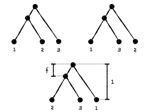
Figure 1: Three species trees.

How is this related to the sparse signal detection problem? Our main goal is to provide a lower bound on the amount of data required for perfect reconstruction, in terms of $m$ (the number of genes) and $k$ (the sequence length). Consider the three possible (rooted, leaf-labelled) species trees with three leaves, as depicted in Figure 1, where we let the time to the most recent divergence be $1-f$ (from today) and the time to the earlier divergence be $1$. Thus $f$ is the time between the two divergence events. In order for a distance-based method to distinguish between these three possibilities, i,e., to determine which pair is closest, we need to estimate the $d_{ab}$s within $O(f)$ accuracy. Put differently, within the multi-locus distance estimation problem, it suffices to establish a lower bound on the data required to distinguish between a two-leaf species tree $S$ with $d_{12}=2$ and a two-leaf species tree $S^{+}$ with $d_{12}=2-2f$, where in both cases $\nu_{e}=1$ for all $e$. We are interested in the limit $f\to 0$.

Let $\mathbb{P}_{0}$ and $\mathbb{Q}$ be the distributions of $\theta(\mathbf{s}^{1}_{1},\mathbf{s}^{1}_{2})$ for a single gene under $S$ and $S^{+}$ respectively, where for ease of notation the dependence on $k$ is implicit. For $m$ genes, we denote the corresponding distributions by $\mathbb{P}_{0}^{\otimes m}$ and $\mathbb{Q}^{\otimes m}$. To connect the problem to sparse signal detection we observe below that, under the multispecies coalescent, $\mathbb{Q}$ is in fact a mixture of $\mathbb{P}_{0}$ and a sparse signal $\mathbb{P}_{1}$, i.e.,

$$\mathbb{Q}=(1-\sigma_{f})\,\mathbb{P}_{0}+\sigma_{f}\,\mathbb{P}_{1},$$ (3)

where $\sigma_{f}=O(f)$ as $f\to 0$.

When testing between $\mathbb{P}_{0}^{\otimes m}$ and $\mathbb{Q}^{\otimes m}$, the optimal sum of Type-I (false positive) and Type-II (false negative) errors is given by (see, e.g., [CT91])

$$\inf_{A}\{\mathbb{P}_{0}^{\otimes m}(A)+\mathbb{Q}^{\otimes m}(A^{c})\}=1-\|\mathbb{P}_{0}^{\otimes m}-\mathbb{Q}^{\otimes m}\|_{\mathrm{TV}},$$ (4)

where $\|\cdot\|_{\mathrm{TV}}$ denotes the total variation distance. Because $\sigma_{f}=O(f)$, for any $k$, in order to distinguish between $\mathbb{P}_{0}$ and $\mathbb{Q}$ one requires that, at the very least, $m=\Omega(f^{-1})$. Otherwise the probability of observing a sample originating from $\mathbb{P}_{1}$ under $\mathbb{Q}$ is bounded away from $1$. In [MR10] it was shown that, provided that $k=\Omega(f^{-2}\log f^{-1})$, $m=\Omega(f^{-1})$ suffices. At the other end of the spectrum, when $k=O(1)$, a lower bound for the single-locus problem obtained by [SS02] implies that $m=\Omega(f^{-2})$ is needed. An algorithm achieving this bound under the multispecies coalescent was recently given in [DNR15].

We settle the full spectrum between these two regimes. Our results apply when $k=f^{-2+2\kappa}$ and $m=f^{-1-\mu}$ where $0<\kappa,\mu<1$ as $f\to 0$.

Theorem 1 (Lower bound).

For any $\delta>0$, there is a $c>0$ such that

$$\|\mathbb{P}_{0}^{\otimes m}-\mathbb{Q}^{\otimes m}\|_{\mathrm{TV}}\leq\delta,$$

whenever

$$m\leq c\frac{1}{f^{2}\sqrt{k}}.$$

Notice that the lower bound on $m$ interpolates between the two extreme regimes discussed above. As $k$ increases, a more accurate estimate of the gene trees can be obtained and one expects that the number of genes required for perfect reconstruction should indeed decrease. The form of that dependence is far from clear however. We in fact prove that our analysis is tight.

Theorem 2 (Matching upper bound).

For any $\delta>0$, there is a $c^{\prime}>0$ such that

$$\|\mathbb{P}_{0}^{\otimes m}-\mathbb{Q}^{\otimes m}\|_{\mathrm{TV}}\geq 1-\delta,$$

whenever

$$m\geq c^{\prime}\frac{1}{f^{2}\sqrt{k}}.$$

Moreover, there is an efficient test to distinguish between $\mathbb{P}_{0}^{\otimes m}$ and $\mathbb{Q}^{\otimes m}$ in that case.

Our proof of the upper bound actually gives an efficient reconstruction algorithm under the molecular clock hypothesis. We expect that the insights obtained from proving Theorem 1 and 2 will lead to more accurate practical methods as well in the general case.

Our results were announced without proof in abstract form in [MR15].

Proof sketch

Let $Z$ be an exponential random variable with mean $1$. We first show that, under $\mathbb{P}_{0}$ (respectively $\mathbb{Q}$), $\theta(\mathbf{s}^{1}_{1},\mathbf{s}^{1}_{2})$ is binomial with $k$ trials and success probability $\frac{3}{4}\left(1-e^{-2(\zeta+Z)}\right)$, where $\zeta=1$ (respectively $\zeta=1-f$). Equation (3) then follows from the memoryless property of the exponential, where $\sigma_{f}$ is the probability that $Z\leq f$.

A recent result of [CW14] gives a formula for the detection boundary of the sparse signal detection problem for general $\mathbb{P}_{0}$, $\mathbb{P}_{1}$. However, applying this formula here is non-trivial. Instead we bound directly the total variation distance between $\mathbb{P}_{0}^{\otimes m}$ and $\mathbb{Q}^{\otimes m}$. Similarly to the approach used in [CW14], we work with the Hellinger distance $H^{2}(\mathbb{P}_{0}^{\otimes m},\mathbb{Q}^{\otimes m})$ which tensorizes as follows (see e.g. [CT91])

$$\frac{1}{2}H^{2}(\mathbb{P}_{0}^{\otimes m},\mathbb{Q}^{\otimes m})=1-\left(1-\frac{1}{2}H^{2}(\mathbb{P}_{0},\mathbb{Q})\right)^{m},$$ (5)

and further satisfies

$$\|\mathbb{P}_{0}^{\otimes m}-\mathbb{Q}^{\otimes m}\|^{2}_{\mathrm{TV}}\leq H^{2}(\mathbb{P}_{0}^{\otimes m},\mathbb{Q}^{\otimes m})\left[1-\frac{1}{4}H^{2}(\mathbb{P}_{0}^{\otimes m},\mathbb{Q}^{\otimes m})\right].$$ (6)

All the work is in proving that, as $f\to 0$,

$$H^{2}(\mathbb{P}_{0},\mathbb{Q})=O\left(f^{2}\sqrt{k}\right).$$

The details are in Section 3.

The proof of Theorem 2 on the other hand involves the construction of a statistical test that distinguishes between $\mathbb{P}_{0}^{\otimes m}$ and $\mathbb{Q}^{\otimes m}$. In the regime $k=O(1)$, an optimal test (up to constants) compares the means of the samples [DNR15]. See also [LYPE09] for a related method (without sample complexity). In the regime $k=\omega(f^{-2})$, an optimal test (up to constants) compares the minima of the samples [MR10]. A natural way to interpolate between these two tests is to consider an appropriate quantile. We show that a quantile of order $1/\sqrt{k}$ leads to the optimal choice.

Organization.

The gene tree generating model is defined in Section 2. The proof of Theorem 1 can be found in Section 3. The proof of Theorem 2 can be found in Section 4.

2 Further definitions

In this section, we give more details on the model.

Some coalescent theory

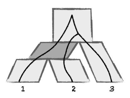
Figure 2: An incomplete lineage sorting event. Although $1$ and $2$ are more closely related in the species tree (fat tree), $2$ and $3$ are more closely related in the gene tree (thin tree). This incongruence is caused by the failure of the lineages originating from $1$ and $2$ to coalesce within the shaded branch.

As we mentioned in the previous section, our gene tree distribution model $\mathcal{G}[S,(\nu_{e},t_{e})_{e\in E}]$ is the multispecies coalescent [RY03]. We first explain the model in the two-species case. Let $1$ and $2$ be two species and consider a common gene $j$. One can trace back in time the lineages of gene $j$ from an individual in $1$ and from an individual in $2$ until the first common ancestor. The latter event is called a coalescence. Here, because the two lineages originate from different species, coalescence occurs in an ancestral population. Let $\tau$ be the time of the divergence between $1$ and $2$ (back in time). Then, under the multispecies coalescent, the coalescence time is $\tau+Z$ where $Z$ is an exponential random variable whose mean depends on the effective population size of the ancestral population. Here we scale time so that the mean is $1$. (See, e.g., [Dur08] for an introduction to coalescent theory.)

We get for the two-level model of sequence data:

Lemma 1 (Distance distribution).

Let $S$ be a two-leaf species tree with $d_{12}=2\tau$ and $\nu_{e}=1$ for all $e$ and let $\theta(\mathbf{s}^{1}_{1},\mathbf{s}^{1}_{2})$ be as in (2) for some $k$. Then the (random) distribution of $\theta(\mathbf{s}^{1}_{1},\mathbf{s}^{1}_{2})$ is binomial with $k$ trials and success probability $\frac{3}{4}\left(1-e^{-2(\tau+Z)}\right)$.

The memoryless property of the exponential gives:

Lemma 2 (Mixture).

Let $S$ be a two-leaf species tree with $d_{12}=2$ and let $S^{+}$ be a two-leaf species tree with $d_{12}=2-2f$, where in both cases $\nu_{e}=1$ for all $e$. Let $\mathbb{P}_{0}$ and $\mathbb{Q}$ be the distributions of $\theta(\mathbf{s}^{1}_{1},\mathbf{s}^{1}_{2})$ for a single gene under $S$ and $S^{+}$ respectively. Then, there is $\mathbb{P}_{1}$ such that,

$$\mathbb{Q}=(1-\sigma_{f})\,\mathbb{P}_{0}+\sigma_{f}\,\mathbb{P}_{1},$$

where $\sigma_{f}=O(f)$, as $f\to 0$.

Proof.

The proof of the lemma is straightforward: We couple perfectly the coalescence time for $\mathbb{Q}$ conditioned on $Z\geq f$ and the unconditional coalescence time for $\mathbb{P}_{0}$ and this extends to a coupling of the distances between the sequences. Thus $\mathbb{P}_{1}$ is obtained by conditioning $\mathbb{Q}$ on the event that $Z$ is $\leq f$ and $\sigma_{f}$ is the probability of that event. ∎

More generally (this paragraph may be skipped as it will not play a role below), consider a species tree $S=(V,E;L,r)$ with $n$ leaves. Each gene $j=1,\ldots,m$ has a genealogical history represented by its gene tree $T_{j}$ distributed according to the following process: looking backwards in time, on each branch of the species tree, the coalescence of any two lineages is exponentially distributed with rate 1, independently from all other pairs; whenever two branches merge in the species tree, we also merge the lineages of the corresponding populations, that is, the coalescence proceeds on the union of the lineages. More specifically, the probability density of a realization of this model for $m$ independent genes is

$$\prod_{j=1}^{m}\prod_{e\in E}\exp\left(-\binom{O_{j}^{e}}{2}\left[\sigma_{j}^{e,O_{j}^{e}+1}-\sigma_{j}^{e,O_{j}^{e}}\right]\right)\prod_{\ell=1}^{I_{j}^{e}-O_{j}^{e}}\exp\left(-\binom{\ell}{2}\left[\sigma_{j}^{e,\ell}-\sigma_{j}^{e,\ell-1}\right]\right),$$

where, for gene $j$ and branch $e$, $I_{j}^{e}$ is the number of lineages entering $e$, $O_{j}^{e}$ is the number of lineages exiting $e$, and $\sigma_{j}^{e,\ell}$ is the $\ell^{th}$ coalescence time in $e$; for convenience, we let $\sigma_{j}^{e,0}$ and $\sigma_{j}^{e,I_{j}^{e}-O_{j}^{e}+1}$ be respectively the divergence times of $e$ and of its parent population. The resulting trees $T_{j}$s may have topologies that differ from that of the species tree $S$. This may occur as a result of an incomplete lineage sorting event, i.e., the failure of two lineages to coalesce in a population. See Figure 2 for an illustration.

A more abstract setting

Before proving Theorem 1, we re-set the problem in a more generic setting that will make the computations more transparent. Let $\mathbb{P}_{0}$ and $\mathbb{P}_{1}$ denote two different distributions for a random variable $X$ supported on $[0,1]$. Given these distributions, we define two distributions, which we will also denote by $\mathbb{P}_{0}$ and $\mathbb{P}_{1}$, for a random variable $\theta$ taking values in $\{0,\ldots,k\}$ for some $k$. These are defined by

$$\mathbb{P}_{i}[\theta=\ell]=\binom{k}{\ell}\mathbb{E}_{i}[X^{\ell}(1-X)^{k-\ell}],$$ (7)

where $\mathbb{E}_{i}$ is the expectation operator corresponding to $\mathbb{P}_{i}$ for the random variable $X$ defined on $[0,1]$. As before, we let

$$\mathbb{Q}=(1-\sigma_{f})\,\mathbb{P}_{0}+\sigma_{f}\,\mathbb{P}_{1},$$

for some $\sigma_{f}=O(f)$. We make the following assumptions which are satisfied in the setting of the previous section.

1. Disjoint supports: $X$ admits a density whose support is $(p_{0},p^{0})$ under $\mathbb{P}_{0}$ and $(p_{0}-\phi_{f},p_{0})$ under $\mathbb{P}_{1}$, where $0<p_{0}<p^{0}<1$ (independent of $f$) and $\phi_{f}=O(f)$. (In the setting of Lemma 2, $p_{0}=\frac{3}{4}(1-e^{-2})$, $p_{0}-\phi_{f}=\frac{3}{4}(1-e^{-(2-2f)})$, and $p^{0}=3/4$.)

2. Bounded density around $p^{0}$: There exist $\rho\in(0,1)$ and $\bar{p}\in(p_{0},p^{0})$, not depending on $f$, such that the following holds. Under $\mathbb{P}_{0}$, the density of $X$ on $(p_{0},\bar{p})$ lies in the interval $[\rho,\rho^{-1}]$, i.e., for any measurable subset $\mathcal{X}\subseteq(p_{0},\bar{p})$ we have

   $$\mathbb{P}_{0}[X\in\mathcal{X}]\in\left[\rho|\mathcal{X}|,\rho^{-1}|\mathcal{X}|\right],$$

   where $|\mathcal{X}|$ is the Lebesgue measure of $\mathcal{X}$. (In the setting of Lemma 2, under $\mathbb{P}_{0}$ the density of $X$ on $(p_{0},p^{0})$ is $\frac{4e^{1/2}}{3}(1-4x/3)^{-3/4}$. Notice that this density is not bounded from below over the entire interval $(p_{0},p^{0})$.)

The first assumption asserts that the supports of $X$ under $\mathbb{P}_{0}$ and $\mathbb{P}_{1}$ are disjoint, while also being highly concentrated under $\mathbb{P}_{1}$ (as $f\to 0$). The key point being that, under $\mathbb{P}_{1}$, $X$ lies near the lower end of the support under $\mathbb{P}_{0}$, which partly explains the effectiveness of a quantile-based test to distinguish between $\mathbb{P}_{0}$ and $\mathbb{Q}$. The second, more technical, assumption asserts that, under $\mathbb{P}_{0}$, the density of $X$ is bounded from above and below in a neighborhood of the lower end of its support. As we will see in Section 3, the dominant contribution to the difference between $\mathbb{P}_{0}$ and $\mathbb{Q}$ comes from the regime where $X$ lies close to $p_{0}$ and we will need to control the probability of observing $X$ there.

3 Lower bound

The proof of the lower bound is based on establishing an upper bound on the Hellinger distance between $\mathbb{P}_{0}$ and $\mathbb{Q}$. The tensoring property of the Hellinger distance then allows to directly obtain an upper bound on the Hellinger distance between $\mathbb{P}_{0}^{\otimes m}$ and $\mathbb{Q}^{\otimes m}$. Using a standard inequality, this finally gives the desired bound on the total variation distance between $\mathbb{P}_{0}^{\otimes m}$ and $\mathbb{Q}^{\otimes m}$.

We first rewrite the Hellinger distance in a form that is convenient for asymptotic expansion. In the abstract setting of Section 2, the Hellinger distance can be written as

$$H^{2}(\mathbb{P}_{0},\mathbb{Q}) = \sum_{j=0}^{k}\left[\sqrt{\mathbb{Q}[\theta=j]}-\sqrt{\mathbb{P}_{0}[\theta=j]}\right]^{2}$$ (8)

$$= \sum_{j=0}^{k}\left[\sqrt{1+\sigma_{f}\left(\frac{\mathbb{P}_{1}[\theta=j]}{\mathbb{P}_{0}[\theta=j]}-1\right)}-1\right]^{2}\mathbb{P}_{0}[\theta=j]$$

$$= \sum_{j=0}^{k}\left[\sqrt{1+\sigma_{f}\left(\frac{\mathbb{E}_{1}[X^{j}(1-X)^{k-j}]}{\mathbb{E}_{0}[X^{j}(1-X)^{k-j}]}-1\right)}-1\right]^{2}\mathbb{P}_{0}[\theta=j]$$

$$= \sum_{j=0}^{k}h_{\sigma_{f}}\left(\frac{\mathbb{E}_{1}[X^{j}(1-X)^{k-j}]}{\mathbb{E}_{0}[X^{j}(1-X)^{k-j}]}\right)\mathbb{P}_{0}[\theta=j],$$

where we define

$$h_{b}(s):=(\sqrt{1+b(s-1)}-1)^{2}.$$ (9)

We will refer to

$$\frac{\mathbb{E}_{1}[X^{j}(1-X)^{k-j}]}{\mathbb{E}_{0}[X^{j}(1-X)^{k-j}]}=\frac{\binom{k}{j}\mathbb{E}_{1}[X^{j}(1-X)^{k-j}]}{\binom{k}{j}\mathbb{E}_{0}[X^{j}(1-X)^{k-j}]}=\frac{\mathbb{P}_{1}[\theta=j]}{\mathbb{P}_{0}[\theta=j]},$$

as the likelihood ratio and to

$$\mathbb{P}_{0}[\theta=j],$$

as the null probability.

We prove the following proposition, which implies Theorem 1.

Proposition 1.

Assume that $k=f^{-2+2\kappa}$ where $0<\kappa<1$ and that Assumptions A1 and A2 hold. As $f\to 0$,

$$H^{2}(\mathbb{P}_{0},\mathbb{Q})=O\left(f^{2}\sqrt{k}\right).$$

The proof of Proposition 1 follows in the next section.

Finally:

Proof of Theorem 1.

The tensorization property of the Hellinger distance, as stated in (5), together with Proposition 1 imply that

$$\frac{1}{2}H^{2}(\mathbb{P}_{0}^{\otimes m},\mathbb{Q}^{\otimes m})=1-\left(1-\frac{1}{2}H^{2}(\mathbb{P}_{0},\mathbb{Q})\right)^{m}=1-\left(1-O\left(f^{2}\sqrt{k}\right)\right)^{m}<\delta,$$

if $m\leq cf^{-2}k^{-1/2}$ for a small enough constant $c$. Thus, by (6), we have

$$\|\mathbb{P}_{0}^{\otimes m}-\mathbb{Q}^{\otimes m}\|^{2}_{\mathrm{TV}}\leq H^{2}(\mathbb{P}_{0}^{\otimes m},\mathbb{Q}^{\otimes m})\left[1-\frac{1}{4}H^{2}(\mathbb{P}_{0}^{\otimes m},\mathbb{Q}^{\otimes m})\right]<\delta,$$

as needed.

∎

3.1 Proof of Proposition 1

From (8), in order to bound the Hellinger distance from above, we need upper bounds on the likelihood ratio $\frac{\mathbb{E}_{1}[X^{j}(1-X)^{k-j}]}{\mathbb{E}_{0}[X^{j}(1-X)^{k-j}]}$ and on the null probability $\mathbb{P}_{0}[\theta=j]$ for each term in the sum. The basic intuition is that the contributions of those terms where $\theta$ is far from its mean under $\mathbb{P}_{1}$ (which is $\approx p_{0}$) are negligible. Indeed:

• When $\theta$ is much smaller than $p_{0}$, the null probability is negligible because, under $\mathbb{P}_{0}$, $X$ is almost surely greater than $p_{0}$. We establish that this leads to an overall contribution to the Hellinger distance of $o(f^{2}\sqrt{k})$. See (21).

• When $\theta$ is much larger than $p_{0}$, the likelihood ratio is negligible because $X$ has a much broader support under $\mathbb{P}_{0}$ than it does under $\mathbb{P}_{1}$. In that case, we show that the overall contribution to the Hellinger distance is $O(f^{2})$. To get a sense of why that is, note that as $f\to 0$

  $$h_{\sigma_{f}}(0)=[\sqrt{1-\sigma_{f}}-1]^{2}=O(f^{2}).$$

  See Claims 1, 2 and 3.

On the other hand, by (7), under both $\mathbb{P}_{0}$ and $\mathbb{P}_{1}$, the random variable $\theta$ conditioned on $X$ is binomial with mean $kX$ and standard deviation of order $\sqrt{k}$. In the regime considered under Theorem 1, i.e., $k=f^{-2+2\kappa}$, we have further that $f=o(1/\sqrt{k})$. Hence by Assumption A1, under $\mathbb{P}_{1}$, $X$ has support of size $O(f)$ and the unconditional random variable $\theta$ also has standard deviation of order $\sqrt{k}$. In this bulk regime, our analysis relies on the following insight:

• How big is each term in the Hellinger sum? In order for $\mathbb{E}_{0}[X^{j}(1-X)^{k-j}]$ to be non-negligible, $X$ must lie within roughly $\sqrt{k}$ of $p_{0}$, which under Assumption A2 has probability $\Theta(1/\sqrt{k})$. On the other hand, under $\mathbb{P}_{1}$, $X$ is almost surely close to $p_{0}$. That produces a likelihood ratio of order $\sqrt{k}$. Therefore, recalling that $f\sqrt{k}=o(1)$, the term

  $$h_{\sigma_{f}}\left(\frac{\mathbb{E}_{1}[X^{j}(1-X)^{k-j}]}{\mathbb{E}_{0}[X^{j}(1-X)^{k-j}]}\right)=\left[\sqrt{1+\sigma_{f}\left(\frac{\mathbb{E}_{1}[X^{j}(1-X)^{k-j}]}{\mathbb{E}_{0}[X^{j}(1-X)^{k-j}]}-1\right)}-1\right]^{2},$$

  is of order $f^{2}k$. Moreover, by the argument above, the overall null probability of the bulk is of order $1/\sqrt{k}$. Thus, we expect that the Hellinger distance in this regime is of order $\sqrt{k}f^{2}$ as stated in Proposition 1. It will be convenient to divide the analysis into $\theta$-values below $p_{0}$ (see Claims 4, 5, 6 and 7) and above $p_{0}$ (see Claims 8, 9, 10 and 11).

The full details are somewhat delicate, as we need to carefully consider various intervals of summands $j$ according to the behavior of the null probability $\mathbb{P}_{0}[\theta=j]$ and the likelihood ratio $\frac{\mathbb{E}_{1}[X^{j}(1-X)^{k-j}]}{\mathbb{E}_{0}[X^{j}(1-X)^{k-j}]}$.

In the next subsection we introduce some notation and prove some simple estimates that will be used in the proofs.

3.2 Some useful lemmas

The following is Lemma 4 in [CW14]:

Lemma 3.

For $b>0$, let $h_{b}(s)=(\sqrt{1+b(s-1)}-1)^{2}$

1. For any $b>0$, the function $h_{b}(s)$ is strictly decreasing on $[0,1]$ and strictly increasing on $[1,+\infty)$.

2. For any $b>0$ and $s\geq 1$,

   $$h_{b}(s)\leq[b(s-1)]\land[b(s-1)]^{2}\leq[bs]\land[bs]^{2}.$$

The following lemmas follow from straightforward calculus.

Lemma 4.

For $j\in\{0,\ldots,k\}$ and $x\in(0,1)$, let

$$\Phi_{j}(x)=\frac{j}{k}\log x+\frac{k-j}{k}\log(1-x).$$

Then

$$\Phi^{\prime}_{j}(x)=\frac{j}{k}\frac{1}{x}-\frac{k-j}{k}\frac{1}{1-x}=\frac{1}{x(1-x)}\left(\frac{j}{k}-x\right).$$

As a result $\Phi_{j}$ is increasing on $[0,\frac{j}{k}]$ and decreasing on $[\frac{j}{k},1]$, and $\Phi^{\prime}_{j}(\frac{j}{k})=0.$

Lemma 5.

For $j\in\{0,\ldots,k\}$, $p\in(0,1)$, and $x\in[0,p)$, let

$$\Psi_{j,p}(x)=\frac{j}{k}\log\frac{p}{p-x}+\frac{k-j}{k}\log\frac{1-p}{1-p+x}.$$

Then:

1. The first two derivatives are:

   $$\Psi^{\prime}_{j,p}(x)=\frac{j}{k}\frac{1}{p-x}-\frac{k-j}{k}\frac{1}{1-p+x}=\frac{1}{(p-x)(1-p+x)}\left(\frac{j}{k}-(p-x)\right),$$

   and

   $$\Psi^{\prime\prime}_{j,p}(x)=\frac{j}{k}\left\{\frac{1}{(p-x)^{2}}\right\}+\frac{k-j}{k}\left\{\frac{1}{(1-p+x)^{2}}\right\}\geq\frac{1}{2},$$

   (since the terms in curly brackets are at least $1$ and one of $\frac{j}{k}$ or $\frac{k-j}{k}$ is greater or equal than $1/2$).

2. By a Taylor expansion around $x=0$, we have for $x\in[0,p)$ and some $x^{*}\in[0,x]$

   $$\Psi_{j,p}(x)=\frac{1}{p(1-p)}\left(\frac{j}{k}-p\right)x+\frac{x^{2}}{2}\Psi^{\prime\prime}_{j,p}(x^{*})\geq\frac{1}{p(1-p)}\left(\frac{j}{k}-p\right)x+\frac{1}{4}x^{2}.$$

3.3 Proof

Let $C$ be a large constant (not depending on $f$) to be determined later. We divide up the sum in (8) into intervals with distinct behaviors. We consider the following intervals for $\frac{j}{k}$:

$$J_{0}=\left[p_{0},p_{0}+C\sqrt{\frac{\log k}{k}}\right],\qquad J_{1}=\left[p_{0}+C\sqrt{\frac{\log k}{k}},1\right],$$

and

$$J^{\prime}_{0} = \left[p_{0}-\phi_{f},p_{0}\right],$$

$$J^{\prime}_{1} = \left[p_{0}-C\sqrt{\frac{\log k}{k}},p_{0}-\phi_{f}\right],$$

$$J^{\prime}_{2} = \left[0,p_{0}-C\sqrt{\frac{\log k}{k}}\right].$$

In words $J_{1}^{\prime}\cup J_{0}^{\prime}\cup J_{0}$ is the bulk of $\mathbb{P}_{1}$, i.e., where $j/k$ sampled from $\mathbb{P}_{1}$ takes its typical values, with $J_{0}^{\prime}$ being the support of $X$ under $\mathbb{P}_{1}$. (This bulk interval is further sub-divided into three intervals whose analyses are slightly different.) The intervals $J_{2}^{\prime}$ and $J_{1}$ are where $j/k$ takes atypically small and large values under $\mathbb{P}_{1}$ respectively. For a subset of $\frac{j}{k}$-values $J$, we write the contribution of $J$ to the Hellinger distance as

$$H^{2}(\mathbb{P}_{0},\mathbb{Q})|_{J}=\sum_{j:j/k\in J}h_{\sigma_{f}}\left(\frac{\mathbb{E}_{1}[X^{j}(1-X)^{k-j}]}{\mathbb{E}_{0}[X^{j}(1-X)^{k-j}]}\right)\mathbb{P}_{0}[\theta=j].$$

Below, it will be convenient to break up the analysis into three regimes: $J_{1}$, which we refer to as the high-substitution regime; $J_{2}^{\prime}\cup J_{1}^{\prime}\cup J_{0}^{\prime}$, the low-substitution regime; and $J_{0}$, the border regime. (Refer back to Section 3.1 for an overview of the proof in these different regimes. Note in particular that we combine the analyses of the atypically low values, $J_{2}^{\prime}$, and the typical values below $p_{0}$, $J_{1}^{\prime}\cup J_{0}^{\prime}$, because they follow from related derivations.)

High substitution regime

We consider $J_{1}$ first. As we previewed in Section 3.1, the argument in this case involves proving that the likelihood ratio is small. Let

$$J_{\leq 1}=\left\{0\leq j\leq k\,:\,\frac{\mathbb{E}_{1}[X^{j}(1-X)^{k-j}]}{\mathbb{E}_{0}[X^{j}(1-X)^{k-j}]}\leq 1\right\}.$$ (10)

I.e., $J_{\leq 1}$ is where the likelihood ratio is bounded by $1$. Note that Lemma 3 in Section 3.2 says that $h_{\sigma_{f}}$ is monotone decreasing in the interval $[0,1]$ and we can therefore bound the sum of terms in $J_{\leq 1}$ assuming the likelihood ratio $\frac{\mathbb{E}_{1}[X^{j}(1-X)^{k-j}]}{\mathbb{E}_{0}[X^{j}(1-X)^{k-j}]}$ in fact equals $0$, as follows,

$$\sum_{j\in J_{\leq 1}}\left[\sqrt{1+\sigma_{f}\left(\frac{\mathbb{E}_{1}[X^{j}(1-X)^{k-j}]}{\mathbb{E}_{0}[X^{j}(1-X)^{k-j}]}-1\right)}-1\right]^{2}\mathbb{P}_{0}[J=j]$$

$$\qquad\leq\sum_{j\in J_{\leq 1}}\left[\sqrt{1-\sigma_{f}}-1\right]^{2}\mathbb{P}_{0}[J=j]$$

$$\qquad=O(\sigma_{f}^{2})$$

$$\qquad=O(f^{2}).$$

We have thus proved the following claim.

Claim 1 (Ratio less than $1$).

$$H^{2}(\mathbb{P}_{0},\mathbb{Q})|_{J_{\leq 1}}=O(f^{2}).$$

Hence, to bound the sum in $J_{1}$, it suffices to show that $J_{1}\subseteq J_{\leq 1}$, which we prove in the next claim.

Claim 2 (High substitution implies ratio less than 1).

It holds that $J_{1}\subseteq J_{\leq 1}$.

Since the support of $X$ under $\mathbb{P}_{1}$ is below $p_{0}$ while it is above $p_{0}$ under $\mathbb{P}_{0}$, we might expect that the likelihood ratio will be bounded by $1$ on $J_{1}$, which is what we prove next.

Proof.

By Assumption A1, under $\mathbb{P}_{1}$, $X$ is a.s. less than $p_{0}$. Since Lemma 4 implies that $\Phi_{j}(x)$ is monotone increasing on $[0,j/k]$, which includes $[0,p_{0}]$ since $\frac{j}{k}\in J_{1}$, it follows that

$$\mathbb{E}_{1}[X^{j}(1-X)^{k-j}] = \mathbb{E}_{1}[\exp(k\Phi_{j}(X))]$$ (11)

$$\leq \exp(k\Phi_{j}(p_{0}))$$

$$= p_{0}^{j}(1-p_{0})^{k-j}.$$

Let $\mathcal{E}$ be the event that

$$\mathcal{E}=\left\{X\in\left[p_{0}+C\sqrt{\frac{\log k}{k}}-\frac{1}{k},p_{0}+C\sqrt{\frac{\log k}{k}}\right]\right\}.$$

By Assumption A2, $\mathbb{P}_{0}[\mathcal{E}]\geq\rho/k$. Hence, using Lemma 4 again, for $\frac{j}{k}\in J_{1}$

$$\mathbb{E}_{0}[X^{j}(1-X)^{k-j}] = \mathbb{E}_{0}[X^{j}(1-X)^{k-j}\,|\,\mathcal{E}]\mathbb{P}_{0}[\mathcal{E}]+\mathbb{E}_{0}[X^{j}(1-X)^{k-j}\,|\,\mathcal{E}^{c}]\mathbb{P}_{0}[\mathcal{E}^{c}]$$ (12)

$$\geq \frac{\rho}{k}p^{j}(1-p)^{k-j},$$

where $p=p_{0}+C\sqrt{\frac{\log k}{k}}-\frac{1}{k}$.

Combining (11) and (12), and using Lemma 5 with $x=p-p_{0}\geq 0$ (for $k>1$ and $C$ large enough), we have

$$\frac{\mathbb{E}_{0}[X^{j}(1-X)^{k-j}]}{\mathbb{E}_{1}[X^{j}(1-X)^{k-j}]} \geq \frac{\rho p^{j}(1-p)^{k-j}}{kp_{0}^{j}(1-p_{0})^{k-j}}$$

$$= \frac{\rho}{k}\exp\left(k\Psi_{j,p}(p-p_{0})\right)$$

$$\geq \frac{\rho}{k}\exp\left(k\left\{\frac{1}{p(1-p)}\left(\frac{j}{k}-p\right)x+\frac{1}{4}x^{2}\right\}\right)$$

$$\geq \frac{\rho}{k}\exp\left(\frac{k}{4}\left(C\sqrt{\frac{\log k}{k}}-\frac{1}{k}\right)^{2}\right)$$

$$\geq \frac{\rho}{k}\exp\left(\frac{C^{2}}{5}\log k\right)$$

$$\geq 1,$$

for $C$ large enough (assuming $k$ is large), where on the fourth line we used that $j/k-p\geq 0$ for $j/k\in J_{1}=\left[p_{0}+C\sqrt{\frac{\log k}{k}},1\right]$. We have thus established $J_{1}\subseteq J_{\leq 1}$ ∎

Combining Claims 1 and 2, we thus obtain:

Claim 3 (High substitution: Hellinger distance).

$$H^{2}(\mathbb{P}_{0},\mathbb{Q})|_{J_{1}}=O(f^{2}).$$

Low substitution regime

In order to estimate the sum in $J^{\prime}_{0}\cup J^{\prime}_{1}\cup J^{\prime}_{2}$ we need to further subdivide it into intervals of doubling length. The basic intuition is that for far enough intervals the null probabilities $\mathbb{P}_{0}[\theta=j]$ are small enough so we can estimate the likelihood ratio term $\frac{\mathbb{E}_{1}[X^{j}(1-X)^{k-j}]}{\mathbb{E}_{0}[X^{j}(1-X)^{k-j}]}$ by its worst value in the interval. However, when the intervals are close to the mean, the fluctuations in $\frac{\mathbb{E}_{1}[X^{j}(1-X)^{k-j}]}{\mathbb{E}_{0}[X^{j}(1-X)^{k-j}]}$ are too big so we need to work with shorter intervals. The partition is defined as follows:

$$I^{\prime}_{0} = \left[p_{0}-\frac{1}{\sqrt{k}},p_{0}\right]$$

$$I^{\prime}_{\ell} = \left[p_{0}-\frac{2^{\ell}}{\sqrt{k}},p_{0}-\frac{2^{\ell-1}}{\sqrt{k}}\right],\qquad\ell\geq 1.$$

Define $L$ by $2^{L}=C\sqrt{\log k}$ (where we may choose $C$ so that it is integer-valued).

We first upper bound $\mathbb{E}_{1}[X^{j}(1-X)^{k-j}]$ using Lemma 4 and Assumption A1:

• On $J^{\prime}_{0}$,

  $$\mathbb{E}_{1}[X^{j}(1-X)^{k-j}] = \mathbb{E}_{1}[\exp(k\Phi_{j}(X))]$$ (13)

  $$\leq \mathbb{E}_{1}[\exp(k\Phi_{j}(j/k))]$$

  $$= (j/k)^{j}(1-j/k)^{k-j}.$$

• On $J^{\prime}_{1}\cup J^{\prime}_{2}$ we have that $X\geq p_{0}-\phi_{f}$ a.s. and therefore

  $$\mathbb{E}_{1}[X^{j}(1-X)^{k-j}]\leq(p_{0}-\phi_{f})^{j}(1-p_{0}+\phi_{f})^{k-j}.$$ (14)

To lower bound $\mathbb{E}_{0}[X^{j}(1-X)^{k-j}]$, we consider the event

$$\mathcal{E}=\left\{X\in\left[p_{0},p_{0}+\sqrt{\frac{1}{k}}\right]\right\}.$$

By Assumption A2 and Lemma 4, on $J^{\prime}_{0}\cup J^{\prime}_{1}\cup J^{\prime}_{2}$, arguing as in (12),

$$\mathbb{E}_{0}[X^{j}(1-X)^{k-j}] \geq \frac{\rho}{\sqrt{k}}p^{j}(1-p)^{k-j},$$ (15)

where $p=p_{0}+\sqrt{\frac{1}{k}}$ (assuming $k$ is large). Combining (13), (14), and (15), and using Lemma 5:

• On $J^{\prime}_{0}$,

  $$\frac{\mathbb{E}_{0}[X^{j}(1-X)^{k-j}]}{\mathbb{E}_{1}[X^{j}(1-X)^{k-j}]} \geq \frac{\rho}{\sqrt{k}}\exp(k\Psi_{j,p}(p-j/k))$$

  $$\geq \frac{\rho}{\sqrt{k}}\exp\left(k\left(-\frac{1}{p(1-p)}\left(\frac{j}{k}-p\right)^{2}+\frac{1}{4}\left(\frac{j}{k}-p\right)^{2}\right)\right)$$

  $$\geq C^{\prime}_{1}\frac{\rho}{\sqrt{k}},$$

  ​for some constant $C^{\prime}_{1}$ (not depending on $f$), where we used that $\phi_{f}\ll\sqrt{1/k}$ so that $\left(\frac{j}{k}-p\right)^{2}=O(1/k)$ and, further, $p(1-p)\in(0,1/4)$.

• On $J^{\prime}_{1}\cup J^{\prime}_{2}$,

  $$\frac{\mathbb{E}_{0}[X^{j}(1-X)^{k-j}]}{\mathbb{E}_{1}[X^{j}(1-X)^{k-j}]}$$

  $$\quad\geq\frac{\rho}{\sqrt{k}}\exp(k\Psi_{j,p}(p-p_{0}+\phi_{f}))$$

  $$\quad\geq\frac{\rho}{\sqrt{k}}\exp\left(k\left(\frac{1}{p(1-p)}\left(\frac{j}{k}-p\right)(p-p_{0}+\phi_{f})+\frac{1}{4}(p-p_{0}+\phi_{f})^{2}\right)\right)$$

  $$\quad\geq\frac{\rho}{\sqrt{k}}\exp\left(-C_{1}\sqrt{k}\left(p-\frac{j}{k}\right)\right)$$

  $$\quad=\frac{\rho}{\sqrt{k}}\exp\left(-C_{1}\sqrt{k}\left(p_{0}+\sqrt{\frac{1}{k}}-\frac{j}{k}\right)\right)$$

  $$\quad=C_{2}\frac{\rho}{\sqrt{k}}\exp\left(-C_{1}\sqrt{k}\left(p_{0}-\frac{j}{k}\right)\right),$$

  ​for some constants $C_{1},C_{2}$ (not depending on $f$), where again we used that $\phi_{f}\ll\sqrt{1/k}$ so that $(p-p_{0}+\phi_{f})^{2}=O(1/k^{2})$.

By decreasing $C_{2}$ appropriately we combine the two bounds into:

Claim 4 (Low substitution: Likelihood ratio).

For all $j/k\in J^{\prime}_{0}\cup J^{\prime}_{1}\cup J^{\prime}_{2}$,

$$\frac{\mathbb{E}_{1}[X^{j}(1-X)^{k-j}]}{\mathbb{E}_{0}[X^{j}(1-X)^{k-j}]}\leq\frac{\sqrt{k}}{C_{2}}\exp\left(C_{1}\sqrt{k}\left(p_{0}-\frac{j}{k}\right)\right).$$ (16)

We now bound the integrand in $H^{2}(\mathbb{P}_{0},\mathbb{Q})$ over $J^{\prime}_{0}\cup J^{\prime}_{1}\cup J^{\prime}_{2}$. As noted after the definition of $J_{\leq 1}$ in equation (10), Lemma 3 implies that on $J_{\leq 1}$

$$h_{\sigma_{f}}\left(\frac{\mathbb{E}_{1}[X^{j}(1-X)^{k-j}]}{\mathbb{E}_{0}[X^{j}(1-X)^{k-j}]}\right)\leq C_{0}f^{2},$$ (17)

for some constant $C_{0}>0$.

• On $J^{\prime}_{0}\cup J^{\prime}_{1}$, we will further use Lemma 3 (Part 2) which, recall, says that for $s\geq 1$ and $b>0$

  $$h_{b}(s)\leq[b(s-1)]\land[b(s-1)]^{2}\leq[bs]\land[bs]^{2}.$$

  In particular observe that, if $s\geq 1$, $b>0$ and $bs<1$, then we have simply $h_{b}(s)\leq[bs]^{2}$. Here $b=\sigma_{f}$ and $s$ is bounded above by the expression in (16). We show first that $bs$ is therefore small. Indeed,

  $$\sigma_{f}\frac{\sqrt{k}}{C_{2}}\exp\left(C_{1}\sqrt{k}\left(p_{0}-\frac{j}{k}\right)\right)=O(f^{\kappa})\exp\left(O(\sqrt{\log f^{-1}})\right)=o(1).$$

  Hence, for those $j/k$-values where the likelihood ratio is bounded below by $1$, we have by Lemma 3 (Part 2) that

  $$h_{\sigma_{f}}\left(\frac{\mathbb{E}_{1}[X^{j}(1-X)^{k-j}]}{\mathbb{E}_{0}[X^{j}(1-X)^{k-j}]}\right)\leq\frac{\sigma^{2}_{f}k}{C_{2}^{2}}\exp\left(2C_{1}\sqrt{k}\left(p_{0}-\frac{j}{k}\right)\right).$$

  For those $j/k$-values where the likelihood ratio is not bounded below by $1$, we instead use (17). Changing the constants we obtain finally the following bound valid on all of on $J^{\prime}_{0}\cup J^{\prime}_{1}$:

  $$h_{\sigma_{f}}\left(\frac{\mathbb{E}_{1}[X^{j}(1-X)^{k-j}]}{\mathbb{E}_{0}[X^{j}(1-X)^{k-j}]}\right)\leq C_{2}f^{2}k\exp\left(C_{1}\sqrt{k}\left(p_{0}-\frac{j}{k}\right)\right).$$ (18)

• On $J^{\prime}_{2}$, arguing as in the previous case, we note that the likelihood ratio multiplied by $\sigma_{f}$ may be larger than $1$ this time. Therefore by Lemma 3 (Part 2) and (17) we have

  $$h_{\sigma_{f}}\left(\frac{\mathbb{E}_{1}[X^{j}(1-X)^{k-j}]}{\mathbb{E}_{0}[X^{j}(1-X)^{k-j}]}\right)$$

  $$\ \ \leq C_{0}f^{2}\lor\left\{\left[\sigma_{f}\frac{\sqrt{k}}{C_{2}}\exp\left(C_{1}\sqrt{k}\left(p_{0}-\frac{j}{k}\right)\right)\right]\land\left[\sigma_{f}\frac{\sqrt{k}}{C_{2}}\exp\left(C_{1}\sqrt{k}\left(p_{0}-\frac{j}{k}\right)\right)\right]^{2}\right\},\qquad\qquad$$

  ​Changing the constants we re-write this expression as

  $$h_{\sigma_{f}}\left(\frac{\mathbb{E}_{1}[X^{j}(1-X)^{k-j}]}{\mathbb{E}_{0}[X^{j}(1-X)^{k-j}]}\right)\leq C_{2}f\sqrt{k}\exp\left(C_{1}\sqrt{k}\left(p_{0}-\frac{j}{k}\right)\right),$$

  where, to upper bound the minimum in square brackets above, we only squared the exponential (which is larger than $1$) and used the fact that $f\sqrt{k}=o(1)$ (which implies that the term $\sigma_{f}\frac{\sqrt{k}}{C_{2}}$ is on the other hand asymptotically smaller than $1$). We also used that $f^{2}<f\sqrt{k}$ to deal with the maximum above.

We combine the two bounds into:

Claim 5 (Low substitution: Integrand).

For all $j/k\in J^{\prime}_{0}\cup J^{\prime}_{1}\cup J^{\prime}_{2}$,

$$h_{\sigma_{f}}\left(\frac{\mathbb{E}_{1}[X^{j}(1-X)^{k-j}]}{\mathbb{E}_{0}[X^{j}(1-X)^{k-j}]}\right)\leq C_{2}(f^{2}k\mathbbm{1}_{j/k\in J^{\prime}_{0}\cup J^{\prime}_{1}}+f\sqrt{k}\mathbbm{1}_{j/k\in J^{\prime}_{2}})\exp\left(C_{1}\sqrt{k}\left(p_{0}-\frac{j}{k}\right)\right).$$ (19)

It remains to bound the integrator, for which we rely on Chernoff’s bound. We let

$$I_{0} = \left[p_{0},p_{0}+\frac{1}{\sqrt{k}}\right]$$

$$I_{\ell} = \left[p_{0}+\frac{2^{\ell-1}}{\sqrt{k}},p_{0}+\frac{2^{\ell}}{\sqrt{k}}\right],\qquad\ell\geq 1.$$

Let $\Lambda>0$ be such that $2^{\Lambda}=(\bar{p}-p_{0})\sqrt{k}$. Then by Assumption A2

$$\mathbb{P}_{0}[\theta/k\in I^{\prime}_{\ell}] = \sum_{\lambda\geq 0}\mathbb{P}_{0}[\theta/k\in I^{\prime}_{\ell}\,|\,X\in I_{\lambda}]\,\mathbb{P}_{0}[X\in I_{\lambda}]$$

$$\leq \sum_{\lambda\geq 0}\mathbb{P}_{0}[\theta/k\in I^{\prime}_{\ell}\,|\,X\in I_{\lambda}]\frac{2^{\lambda-1}}{\sqrt{k}}\rho^{-1}+\sum_{\lambda>\Lambda}\mathbb{P}_{0}[\theta/k\in I^{\prime}_{\ell}\,|\,X\in I_{\lambda}].$$

By Chernoff’s bound

$$\mathbb{P}_{0}[\theta/k\in I^{\prime}_{\ell}\,|\,X\in I_{\lambda}]\leq\exp\left(-2(2^{\ell-1}+2^{\lambda-1})^{2}\right)\leq\exp\left(-2^{2\ell-1}-2^{2\lambda-1}\right).$$

In particular

$$\sum_{\lambda>\Lambda}\mathbb{P}_{0}[\theta/k\in I^{\prime}_{\ell}\,|\,X\in I_{\lambda}] \leq \exp\left(-2^{2\ell-1}\right)\sum_{\lambda>\Lambda}\exp\left(-2^{2\lambda-1}\right)$$

$$\leq \exp\left(-2^{2\ell-1}\right)\exp\left(-C^{\prime}_{3}k\right),$$

for some constant $C^{\prime}_{3}>0$ (not depending on $f$). On the other hand,

$$\sum_{\lambda\geq 0}\mathbb{P}_{0}[\theta/k\in I^{\prime}_{\ell}\,|\,X\in I_{\lambda}]\frac{2^{\lambda-1}}{\sqrt{k}}\rho^{-1} \leq \frac{\exp\left(-2^{2\ell-1}\right)}{\rho\sqrt{k}}\sum_{\lambda\geq 0}2^{\lambda-1}\exp\left(-2^{2\lambda-1}\right)$$

$$\leq \frac{C_{3}\exp\left(-2^{2\ell-1}\right)}{\sqrt{k}},$$

for a constant $C_{3}>0$ (not depending on $f$). Combining the bounds and increasing $C_{3}$ appropriately, we get

Claim 6 (Low substitution: Integrator).

For all $\ell\geq 0$,

$$\mathbb{P}_{0}[\theta/k\in I^{\prime}_{\ell}]\leq\frac{C_{3}\exp\left(-2^{2\ell-1}\right)}{\sqrt{k}}.$$ (20)

We can now compute the contribution of $J^{\prime}_{0}\cup J^{\prime}_{1}\cup J^{\prime}_{2}$ to the Hellinger distance. Recall that $L$ is defined by $2^{L}=C\sqrt{\log k}$. From (19) and (20), we get:

• For $0\leq\ell\leq L$,

  $$H^{2}(\mathbb{P}_{0},\mathbb{Q})|_{I^{\prime}_{\ell}} \leq C_{2}f^{2}k\exp\left(C_{1}\sqrt{k}\left(\frac{2^{\ell}}{\sqrt{k}}\right)\right)\frac{C_{3}\exp\left(-2^{2\ell-1}\right)}{\sqrt{k}}$$

  $$\leq C_{2}C_{3}f^{2}\sqrt{k}\exp\left(-2^{2\ell-1}+C_{1}2^{\ell}\right)$$

  $$\leq C_{5}f^{2}\sqrt{k}\exp\left(-C_{4}2^{2\ell}\right),$$

  for some constants $C_{4},C_{5}>0$. Summing over $\ell$ we get

  $$\sum_{\ell=0}^{L}H^{2}(\mathbb{P}_{0},\mathbb{Q})|_{I^{\prime}_{\ell}}\leq C_{6}f^{2}\sqrt{k},$$

  for some constant $C_{6}>0$.

• Similarly, for $\ell>L$,

  $$H^{2}(\mathbb{P}_{0},\mathbb{Q})|_{I^{\prime}_{\ell}} \leq C_{5}f\exp\left(-C_{4}2^{2\ell}\right),$$

  adapting constants $C_{4},C_{5}>0$. Summing over $\ell$ we get

  $$\sum_{\ell>L}H^{2}(\mathbb{P}_{0},\mathbb{Q})|_{I^{\prime}_{\ell}}\leq C_{8}f\exp\left(-C_{7}C^{2}\log k\right)=o(f^{1+\kappa})=o(f^{2}\sqrt{k}),$$ (21)

  by choosing $C$ large enough.

Combining these bounds we get finally:

Claim 7 (Low substitution: Hellinger distance).

$$H^{2}(\mathbb{P}_{0},\mathbb{Q})|_{J^{\prime}_{0}\cup J^{\prime}_{1}\cup J^{\prime}_{2}}=O(f^{2}\sqrt{k}).$$

Border regime.

We now consider $J_{0}$, i.e., the bulk regime above $p_{0}$. The high-level argument is similar to the case of $J_{0}^{\prime}\cup J_{1}^{\prime}$ above, although some details differ. We first bound $\mathbb{E}_{1}[X^{j}(1-X)^{k-j}]$ using Lemma 4 and Assumption A1

$$\mathbb{E}_{1}[X^{j}(1-X)^{k-j}]\leq p_{0}^{j}(1-p_{0})^{k-j}.$$ (22)

To bound $\mathbb{E}_{0}[X^{j}(1-X)^{k-j}]$, we consider the event

$$\mathcal{E}=\left\{X\in\left[\frac{j}{k},\frac{j}{k}+\sqrt{\frac{1}{k}}\right]\right\}.$$

By Assumption A2 and Lemma 4, on $J_{0}$, arguing as in (12),

$$\mathbb{E}_{0}[X^{j}(1-X)^{k-j}] \geq \frac{\rho}{\sqrt{k}}p^{j}(1-p)^{k-j},$$ (23)

where $p=\frac{j}{k}+\sqrt{\frac{1}{k}}$. Combining (22) and (23), and using Lemma 5, on $J_{0}$,

$$\frac{\mathbb{E}_{0}[X^{j}(1-X)^{k-j}]}{\mathbb{E}_{1}[X^{j}(1-X)^{k-j}]} \geq \frac{\rho}{\sqrt{k}}\exp(k\Psi_{j,p}(p-p_{0}))$$

$$\geq \frac{\rho}{\sqrt{k}}\exp\left(k\left(\frac{1}{p(1-p)}\left(\frac{j}{k}-p\right)(p-p_{0})+\frac{1}{4}(p-p_{0})^{2}\right)\right).$$

​For $j/k\in I_{\ell}$, $\ell\leq L$,

$$\frac{\mathbb{E}_{0}[X^{j}(1-X)^{k-j}]}{\mathbb{E}_{1}[X^{j}(1-X)^{k-j}]} \geq \frac{\rho}{\sqrt{k}}\exp\left(k\left(-\frac{1}{p(1-p)}\sqrt{\frac{1}{k}}\left(\frac{2^{\ell}+1}{\sqrt{k}}\right)+\frac{1}{4}\left(\frac{2^{\ell-1}+1}{\sqrt{k}}\right)^{2}\right)\right)$$

$$\geq C_{2}\frac{1}{\sqrt{k}}\exp\left(C_{1}2^{2\ell}\right),$$

​for constants $C_{1},C_{2}>0$.

Claim 8 (Border regime: Likelihood ratio).

For all $j/k\in I_{\ell}$, $\ell\leq L$,

$$\frac{\mathbb{E}_{1}[X^{j}(1-X)^{k-j}]}{\mathbb{E}_{0}[X^{j}(1-X)^{k-j}]}\leq\frac{\sqrt{k}}{C_{2}}\exp\left(-C_{1}2^{2\ell}\right).$$ (24)

We now bound the integrand in $H^{2}(\mathbb{P}_{0},\mathbb{Q})$. We follow the argument leading up to (18). Because $\sigma_{f}\sqrt{k}=o(1),$ by Lemma 3 (Part 2) and (17) we have on $I_{\ell}$

$$h_{\sigma_{f}}\left(\frac{\mathbb{E}_{1}[X^{j}(1-X)^{k-j}]}{\mathbb{E}_{0}[X^{j}(1-X)^{k-j}]}\right)\leq C_{0}f^{2}\lor\frac{\sigma^{2}_{f}k}{C_{2}^{2}}\exp\left(-2C_{1}2^{2\ell}\right).$$

Changing the constants we re-write this expression as

$$h_{\sigma_{f}}\left(\frac{\mathbb{E}_{1}[X^{j}(1-X)^{k-j}]}{\mathbb{E}_{0}[X^{j}(1-X)^{k-j}]}\right)\leq C_{0}f^{2}\lor C_{2}f^{2}k\exp\left(-C_{1}2^{2\ell}\right).$$

Claim 9 (Border regime: Integrand).

For all $j/k\in I_{\ell}$, $0\leq\ell\leq L$,

$$h_{\sigma_{f}}\left(\frac{\mathbb{E}_{1}[X^{j}(1-X)^{k-j}]}{\mathbb{E}_{0}[X^{j}(1-X)^{k-j}]}\right)\leq C_{0}f^{2}\lor C_{2}f^{2}k\exp\left(-C_{1}2^{2\ell}\right).$$ (25)

It remains to bound the integrator. We have by Assumption A2 (recall that $2^{\Lambda}=(\bar{p}-p_{0})\sqrt{k}$)

$$\mathbb{P}_{0}[\theta/k\in I_{\ell}] = \sum_{\lambda\geq 0}\mathbb{P}_{0}[\theta/k\in I_{\ell}\,|\,X\in I_{\lambda}]\mathbb{P}_{0}[X\in I_{\lambda}]$$

$$\leq \sum_{0\leq\lambda\leq\ell}\mathbb{P}_{0}[X\in I_{\lambda}]+\sum_{\ell<\lambda\leq\Lambda}\mathbb{P}_{0}[\theta/k\in I_{\ell}\,|\,X\in I_{\lambda}]\mathbb{P}_{0}[X\in I_{\lambda}]$$

$$\qquad+\sum_{\lambda>\Lambda}\mathbb{P}_{0}[\theta/k\in I_{\ell}\,|\,X\in I_{\lambda}]$$

$$\leq \frac{2^{\ell}}{\sqrt{k}}\rho^{-1}+\sum_{\ell<\lambda\leq\Lambda}\mathbb{P}_{0}[\theta/k\in I_{\ell}\,|\,X\in I_{\lambda}]\frac{2^{\lambda-1}}{\sqrt{k}}\rho^{-1}$$

$$\qquad+\sum_{\lambda>\Lambda}\mathbb{P}_{0}[\theta/k\in I_{\ell}\,|\,X\in I_{\lambda}].$$

By Chernoff’s bound, for $\lambda>\ell$,

$$\mathbb{P}_{0}[\theta/k\in I_{\ell}\,|\,X\in I_{\lambda}]\leq\exp\left(-2(-2^{\ell}+2^{\lambda-1})^{2}\right)\leq\exp\left(-2^{2\ell+1}(2^{\lambda-\ell-1}-1)^{2}\right).$$

In particular

$$\sum_{\lambda>\Lambda}\mathbb{P}_{0}[\theta/k\in I_{\ell}\,|\,X\in I_{\lambda}] \leq \exp\left(-C^{\prime}_{3}k\right),$$

for some constant $C^{\prime}_{3}>0$ (not depending on $f$). On the other hand,

$$\sum_{\ell<\lambda\leq\Lambda}\mathbb{P}_{0}[\theta/k\in I_{\ell}\,|\,X\in I_{\lambda}]\frac{2^{\lambda-1}}{\sqrt{k}}\rho^{-1} \leq \frac{C_{3}2^{\ell}}{\sqrt{k}},$$

for a constant $C_{3}>0$ (not depending on $f$). Combining the bounds and increasing $C_{3}$ appropriately, we get

Claim 10 (Border substitution: Integrator).

For all $0\leq\ell<L$,

$$\mathbb{P}_{0}[\theta/k\in I_{\ell}]\leq\frac{C_{3}2^{\ell}}{\sqrt{k}}.$$ (26)

We can now compute the contribution of $J_{0}$ to the Hellinger distance. From (25) and (26), we get for $0\leq\ell\leq L$

$$H^{2}(\mathbb{P}_{0},\mathbb{Q})|_{I_{\ell}} \leq \left[C_{0}f^{2}\lor C_{2}f^{2}k\exp\left(-C_{1}2^{2\ell}\right)\right]\frac{C_{3}2^{\ell}}{\sqrt{k}}.$$

Summing over $\ell$ we get

$$\sum_{\ell=0}^{L}H^{2}(\mathbb{P}_{0},\mathbb{Q})|_{I_{\ell}}\leq C_{4}f^{2}\sqrt{k},$$

for some constant $C_{4}>0$.

Claim 11 (Border regime: Hellinger distance).

$$H^{2}(\mathbb{P}_{0},\mathbb{Q})|_{J_{0}}=O(f^{2}\sqrt{k}).$$

Wrapping up

We now prove Proposition 1.

Proof of Proposition 1.

$$H^{2}(\mathbb{P}_{0},\mathbb{Q})\leq H^{2}_{J_{1}}(\mathbb{P}_{0},\mathbb{Q})+H^{2}_{J_{0}^{\prime}\cup J_{1}^{\prime}\cup J_{2}^{\prime}}(\mathbb{P}_{0},\mathbb{Q})+H^{2}_{J_{0}}(\mathbb{P}_{0},\mathbb{Q})\leq O(f^{2}\sqrt{k}),$$

by Claims 3, 7 and 11. That implies Proposition 1. ∎

4 Matching upper bound

We give two proofs of the upper bound.

4.1 Proof of Theorem 2

Proof.

We use (4) and construct an explicit test $A$ as follows:

• Let $W$ be the number of genes such that $\theta/k\leq p_{0}$. Let $w=\mathbb{P}_{0}[\theta/k\leq p_{0}]$, $w^{\prime}=\mathbb{Q}[\theta/k\leq p_{0}]$ and

  $$w^{*}=m\frac{w+w^{\prime}}{2}=mw+\frac{m}{2}(w^{\prime}-w)=mw^{\prime}-\frac{m}{2}(w^{\prime}-w).$$

  We consider the following event

  $$A=\{W\geq w^{*}\}.$$

It remains to show that the event $A$ is highly unlikely under $\mathbb{P}_{0}^{\otimes m}$ while being highly likely under $\mathbb{Q}^{\otimes m}$. We do this by bounding the difference $w^{\prime}-w$ and applying Chebyshev’s inequality to $W$.

Note that $W\sim\mathrm{Bin}(m,w)$ under $\mathbb{P}_{0}^{\otimes m}$ and $W\sim\mathrm{Bin}(m,w^{\prime})$ under $\mathbb{Q}^{\otimes m}$. By Assumption A1, $X\in[p_{0}-\phi_{f},p_{0}]$ under $\mathbb{P}_{1}$. By the Berry-Esseen theorem (e.g. [Dur96]),

$$\mathbb{P}_{1}[\theta/k\leq p_{0}]\geq\mathbb{E}_{1}[\mathbb{P}_{1}[\theta\leq kX\,|\,X]]=\frac{1}{2}-O\left(\frac{1}{\sqrt{k}}\right)\geq\frac{1}{3},$$ (27)

for $k$ large enough. Hence,

$$w^{\prime} = \sigma_{f}\mathbb{P}_{1}[\theta/k\leq p_{0}]+(1-\sigma_{f})w$$ (28)

$$\geq \frac{1}{3}\sigma_{f}+(1-\sigma_{f})w,$$

whereas by the computations in the previous section (more specifically, by summing over $\ell$ in (20))

$$w=O\left(\frac{1}{\sqrt{k}}\right),$$ (29)

and, similarly, since $f\sqrt{k}=o(1)$

$$w^{\prime}=O\left(\frac{1}{\sqrt{k}}\right),$$ (30)

from (28) and (29). Consequently

$$w^{\prime}-w\geq\sigma_{f}\left(\frac{1}{3}-w\right)=\Omega(f).$$ (31)

By Chebyshev’s inequality,

$$\mathbb{P}_{0}^{\otimes m}\left[A\right]\leq\frac{4mw(1-w)}{m^{2}(w^{\prime}-w)^{2}}=O\left(\frac{1}{mf^{2}\sqrt{k}}\right)\leq\frac{\delta}{2},$$

for $c^{\prime}$ large enough, where we used (29) and (31). Similarly,

$$\mathbb{Q}^{\otimes m}\left[A^{c}\right]\leq\frac{4mw^{\prime}(1-w^{\prime})}{m^{2}(w^{\prime}-w)^{2}}\leq\frac{\delta}{2}.$$

∎

4.2 Agnostic version

Although Theorem 2 shows that our bound in Theorem 1 is tight, it relies on a test (i.e., the set $A$) that assumes knowledge of the null and alternative hypotheses. Here we relax this assumption.

Pairwise distance comparisons

We assume that we have two (independent) collections of genes, $\mathcal{T}_{1}$ and $\mathcal{T}_{2}$, one from each model, $\mathbb{P}_{0}$ and $\mathbb{Q}$ as in the previous section. We split the genes into two equal-sized disjoint sub-collections, $(\mathcal{T}_{1}^{1},\mathcal{T}_{1}^{2})$ and $(\mathcal{T}_{2}^{1},\mathcal{T}_{2}^{2})$. Assume for convenience that the total number of genes is in fact $2m$ for each dataset. Let $C>0$ be a constant, to be determined later (in equation (33)). We proceed in two steps.

1. We first compute $\hat{p}_{1}$ and $\hat{p}_{2}$, the $\frac{C}{\sqrt{k}}$-quantiles based on $\mathcal{T}_{1}^{1}$ and $\mathcal{T}_{2}^{1}$ respectively. Let $\hat{p}=\max\{\hat{p}_{1},\hat{p}_{2}\}$.

2. Compute the fraction of genes, $\hat{w}_{1}$ and $\hat{w}_{2}$, with $\theta/k\leq\hat{p}$ in $\mathcal{T}_{1}^{2}$ and $\mathcal{T}_{2}^{2}$ respectively.

We infer that the first dataset comes from $\mathbb{P}_{0}^{\otimes 2m}$ if $\hat{w}_{1}<\hat{w}_{2}$, and vice versa.

Remark 1.

Simply comparing the $\frac{C}{\sqrt{k}}$-quantiles breaks down when $f\ll\frac{1}{k}$, as it is quite possible that the quantiles will be identical since they can only take $k$ possible values. However, even if the quantiles are identical, the probability of a gene being lower than the quantile is bigger if the distance is smaller. This explains the need for the second phase in our algorithm. We remark further that the partition of the data into two sets is used for analysis purposes as it allows for better control of dependencies.

We show that this approach succeeds with probability at least $1-\delta$ whenever $m\geq c^{\prime}\frac{1}{f^{2}\sqrt{k}}$, for $c^{\prime}$ large enough. This proceeds from a series of claims.

Claim 12 ($\hat{p}$ is close to $p_{0}$).

For $c^{\prime}$ large enough, there is $C_{1}>0$ such that

$$\hat{p}\in\left[p_{0},p_{0}+\frac{C_{1}}{\sqrt{k}}\right]$$ (32)

with probability $1-\delta/2$.

Proof.

The argument is similar to that in the proof of Theorem 2.

By summing over $\ell$ in (20),

$$\mathbb{P}_{0}[\theta/k\leq p_{0}]\leq\frac{C^{\prime}_{1}}{\sqrt{k}},$$

for some $C_{1}^{\prime}>0$. For any $C^{\prime\prime}_{1}>C^{\prime}_{1}$, there is $C_{1}>0$ such that

$$\mathbb{P}_{0}\left[\theta/k\leq p_{0}+\frac{C_{1}}{\sqrt{k}}\right] \geq \mathbb{P}_{0}\left[\theta/k\leq p_{0}+\frac{C_{1}}{\sqrt{k}}\,\bigg{|}\,X\in\left[p_{0},p_{0}+\frac{C_{1}}{\sqrt{k}}\right]\right]$$

$$\qquad\qquad\qquad\qquad\times\,\mathbb{P}_{0}\left[X\in\left[p_{0},p_{0}+\frac{C_{1}}{\sqrt{k}}\right]\right]$$

$$\geq \frac{1}{3}\frac{\rho\,C_{1}}{\sqrt{k}}\geq\frac{C_{1}^{\prime\prime}}{\sqrt{k}}$$

by the Berry-Esseen theorem (as in (27)), for $C_{1}$ large enough.

Let

$$C=\frac{C^{\prime}_{1}+C^{\prime\prime}_{1}}{2}.$$ (33)

Let $W$ be the number of genes (among $m$) such that $\theta/k\leq p_{0}$ and $w=\mathbb{P}_{0}[\theta/k\leq p_{0}]$. Repeating the calculations in the proof of Theorem 2,

$$\mathbb{P}_{0}^{\otimes m}\left[W\geq m\frac{C}{\sqrt{k}}\right]\leq\frac{4mw(1-w)k}{m^{2}(C-C_{1}^{\prime})^{2}}=\frac{1}{m}O\left(\sqrt{k}\right)\leq\frac{1}{c^{\prime}}O(f^{2}k)\leq\frac{\delta}{8},$$

for $c^{\prime}$ large enough. Similarly, let $\tilde{W}$ be the number of genes such that $\theta/k\leq p_{0}+C_{1}/\sqrt{k}$ and $\tilde{w}=\mathbb{P}_{0}[\theta/k\leq p_{0}+C_{1}/\sqrt{k}]$. Then

$$\mathbb{P}_{0}^{\otimes m}\left[\tilde{W}\leq m\frac{C}{\sqrt{k}}\right]\leq\frac{\delta}{8}.$$

That implies that with probability $1-\delta/4$ the $C/\sqrt{k}$-quantile under $\mathbb{P}_{0}^{\otimes m}$ lies in the interval $[p_{0},p_{0}+\frac{C_{1}}{\sqrt{k}}]$. By monotonicity, $\mathbb{P}_{1}[\theta/k\leq p_{0}+C_{1}/\sqrt{k}]\geq\tilde{w}$, and we also have

$$\mathbb{Q}^{\otimes m}\left[\tilde{W}\leq m\frac{C}{\sqrt{k}}\right]\leq\frac{\delta}{8},$$

which implies the claim. ∎

Claim 13 (Test).

For $c^{\prime}$ large enough, if $\mathcal{T}_{1}$ comes from $\mathbb{P}_{0}^{\otimes 2m}$, $\mathcal{T}_{2}$ comes from $\mathbb{Q}^{\otimes 2m}$ and (32) holds, then

$$\hat{w}_{1}<\hat{w}_{2}$$

with probability $1-\delta/2$, and vice versa.

Proof.

The proof is identical to that of Theorem 2 with $W$ now being the number of genes such that $\theta/k\leq\hat{p}$, $w=\mathbb{P}_{0}[\theta/k\leq\hat{p}]$, $w^{\prime}=\mathbb{Q}[\theta/k\leq\hat{p}]$, and (29) and (30) now following from Claim 12 together with (20) and (26). ∎

Triplet reconstruction

Consider again the three possible species trees depicted in Figure 2. By comparing the pairs two by two as described in the agnostic algorithm, we can determine which is the correct species tree topology. Such “triplet” information is in general enough (assuming the molecular clock hypothesis) to reconstruct a species tree on any number of species (e.g. [SS03]). We leave out the details.

References

• [ADHR12] Alexandr Andoni, Constantinos Daskalakis, Avinatan Hassidim, and Sebastien Roch. Global alignment of molecular sequences via ancestral state reconstruction. Stochastic Processes and their Applications, 122(12):3852 – 3874, 2012.
• [ADR11] Elizabeth S. Allman, James H. Degnan, and John A. Rhodes. Identifying the rooted species tree from the distribution of unrooted gene trees under the coalescent. Journal of Mathematical Biology, 62(6):833–862, 2011.
• [ALPE12] Christian N.K. Anderson, Liang Liu, Dennis Pearl, and Scott V. Edwards. Tangled trees: The challenge of inferring species trees from coalescent and noncoalescent genes. In Maria Anisimova, editor, Evolutionary Genomics, volume 856 of Methods in Molecular Biology, pages 3–28. Humana Press, 2012.
• [BS14] Anand Bhaskar and Yun S. Song. Descartes’ rule of signs and the identifiability of population demographic models from genomic variation data. Ann. Statist., 42(6):2469–2493, 2014.
• [CGG02] M. Cryan, L. A. Goldberg, and P. W. Goldberg. Evolutionary trees can be learned in polynomial time. SIAM J. Comput., 31(2):375–397, 2002.
• [CJJ11] T. Tony Cai, X. Jessie Jeng, and Jiashun Jin. Optimal detection of heterogeneous and heteroscedastic mixtures. J. R. Stat. Soc. Ser. B Stat. Methodol., 73(5):629–662, 2011.
• [CJT05] L. Cayon, J. Jin, and A. Treaster. Higher criticism statistic: detecting and identifying non-gaussianity in the wmap first-year data. Monthly Notices of the Royal Astronomical Society, 362(3):826–832, 2005.
• [CT91] T. M. Cover and J. A. Thomas. Elements of information theory. Wiley Series in Telecommunications. John Wiley & Sons Inc., New York, 1991. A Wiley-Interscience Publication.
• [CW14] T.T. Cai and Yihong Wu. Optimal detection of sparse mixtures against a given null distribution. Information Theory, IEEE Transactions on, 60(4):2217–2232, April 2014.
• [DBP05] Frederic Delsuc, Henner Brinkmann, and Herve Philippe. Phylogenomics and the reconstruction of the tree of life. Nat Rev Genet, 6(5):361–375, 05 2005.
• [DD10] Michael DeGiorgio and James H Degnan. Fast and consistent estimation of species trees using supermatrix rooted triples. Molecular Biology and Evolution, 27(3):552–69, March 2010.
• [DDBR09] James H. Degnan, Michael DeGiorgio, David Bryant, and Noah A. Rosenberg. Properties of consensus methods for inferring species trees from gene trees. Systematic Biology, 58(1):35–54, 2009.
• [DJ04] David Donoho and Jiashun Jin. Higher criticism for detecting sparse heterogeneous mixtures. Ann. Statist., 32(3):962–994, 06 2004.
• [DMR11a] Constantinos Daskalakis, Elchanan Mossel, and Sébastien Roch. Evolutionary trees and the ising model on the bethe lattice: a proof of steel’s conjecture. Probability Theory and Related Fields, 149:149–189, 2011. 10.1007/s00440-009-0246-2.
• [DMR11b] Constantinos Daskalakis, Elchanan Mossel, and Sébastien Roch. Phylogenies without branch bounds: Contracting the short, pruning the deep. SIAM J. Discrete Math., 25(2):872–893, 2011.
• [DNR15] Gautam Dasarathy, Robert D. Nowak, and Sébastien Roch. Data requirement for phylogenetic inference from multiple loci: A new distance method. IEEE/ACM Trans. Comput. Biology Bioinform., 12(2):422–432, 2015.
• [Dob58] R. L. Dobrusin. A statistical problem arising in the theory of detection of signals in the presence of noise in a multi-channel system and leading to stable distribution laws. Theory of Probability & Its Applications, 3(2):161–173, 1958.
• [DR06] J. H. Degnan and N. A. Rosenberg. Discordance of species trees with their most likely gene trees. PLoS Genetics, 2(5), May 2006.
• [DR09] James H. Degnan and Noah A. Rosenberg. Gene tree discordance, phylogenetic inference and the multispecies coalescent. Trends in Ecology and Evolution, 24(6):332 – 340, 2009.
• [DR13] Constantinos Daskalakis and Sebastien Roch. Alignment-free phylogenetic reconstruction: sample complexity via a branching process analysis. Ann. Appl. Probab., 23(2):693–721, 2013.
• [Dur96] Richard Durrett. Probability: theory and examples. Duxbury Press, Belmont, CA, second edition, 1996.
• [Dur08] Richard Durrett. Probability models for DNA sequence evolution. Probability and its Applications (New York). Springer, New York, second edition, 2008.
• [ESSW99a] P. L. Erdös, M. A. Steel;, L. A. Székely, and T. A. Warnow. A few logs suffice to build (almost) all trees (part 1). Random Struct. Algor., 14(2):153–184, 1999.
• [ESSW99b] P. L. Erdös, M. A. Steel;, L. A. Székely, and T. A. Warnow. A few logs suffice to build (almost) all trees (part 2). Theor. Comput. Sci., 221:77–118, 1999.
• [Fel04] J. Felsenstein. Inferring Phylogenies. Sinauer, New York, New York, 2004.
• [HTF09] Trevor Hastie, Robert Tibshirani, and Jerome Friedman. The elements of statistical learning. Springer Series in Statistics. Springer, New York, second edition, 2009. Data mining, inference, and prediction.
• [Ing97] Yu. I. Ingster. Some problems of hypothesis testing leading to infinitely divisible distributions. Math. Methods Statist., 6(1):47–69, 1997.
• [JC69] T. H. Jukes and C. Cantor. Mammalian protein metabolism. In H. N. Munro, editor, Evolution of protein molecules, pages 21–132. Academic Press, 1969.
• [JCL10] X. Jessie Jeng, T. Tony Cai, and Hongzhe Li. Optimal sparse segment identification with application in copy number variation analysis. J. Amer. Statist. Assoc., 105(491):1156–1166, 2010.
• [KHH+05] Martin Kulldorff, Richard Heffernan, Jessica Hartman, Renato Assun o, and Farzad Mostashari. A space?time permutation scan statistic for disease outbreak detection. PLoS Med, 2(3):e59, 02 2005.
• [KMRR15] Junhyong Kim, Elchanan Mossel, Mikl s Z. R cz, and Nathan Ross. Can one hear the shape of a population history? Theoretical Population Biology, 100(0):26 – 38, 2015.
• [LYK+09] Liang Liu, Lili Yu, Laura Kubatko, Dennis K. Pearl, and Scott V. Edwards. Coalescent methods for estimating phylogenetic trees. Molecular Phylogenetics and Evolution, 53(1):320 – 328, 2009.
• [LYP10] Liang Liu, Lili Yu, and DennisK. Pearl. Maximum tree: a consistent estimator of the species tree. Journal of Mathematical Biology, 60(1):95–106, 2010.
• [LYPE09] Liang Liu, Lili Yu, Dennis K. Pearl, and Scott V. Edwards. Estimating species phylogenies using coalescence times among sequences. Systematic Biology, 58(5):468–477, 2009.
• [Mad97] Wayne P. Maddison. Gene trees in species trees. Systematic Biology, 46(3):523–536, 1997.
• [MFP08] Simon Myers, Charles Fefferman, and Nick Patterson. Can one learn history from the allelic spectrum? Theoretical Population Biology, 73(3):342 – 348, 2008.
• [Mos03] E. Mossel. On the impossibility of reconstructing ancestral data and phylogenies. J. Comput. Biol., 10(5):669–678, 2003.
• [Mos04] E. Mossel. Phase transitions in phylogeny. Trans. Amer. Math. Soc., 356(6):2379–2404, 2004.
• [MR06] Elchanan Mossel and Sébastien Roch. Learning nonsingular phylogenies and hidden Markov models. Ann. Appl. Probab., 16(2):583–614, 2006.
• [MR10] Elchanan Mossel and Sébastien Roch. Incomplete lineage sorting: Consistent phylogeny estimation from multiple loci. IEEE/ACM Trans. Comput. Biology Bioinform., 7(1):166–171, 2010.
• [MR15] Elchanan Mossel and Sébastien Roch. Distance-based species tree estimation: Information-theoretic trade-off between number of loci and sequence length under the coalescent. In Approximation, Randomization, and Combinatorial Optimization. Algorithms and Techniques, APPROX/RANDOM 2015, August 24-26, 2015, Princeton, NJ, USA, pages 931–942, 2015.
• [MRS11] Elchanan Mossel, Sébastien Roch, and Allan Sly. On the inference of large phylogenies with long branches: How long is too long? Bulletin of Mathematical Biology, 73:1627–1644, 2011. 10.1007/s11538-010-9584-6.
• [MSZ+13] Raphaël Mourad, Christine Sinoquet, Nevin Lianwen Zhang, Tengfei Liu, and Philippe Leray. A survey on latent tree models and applications. J. Artif. Intell. Res. (JAIR), 47:157–203, 2013.
• [Nak13] Luay Nakhleh. Computational approaches to species phylogeny inference and gene tree reconciliation. Trends in ecology & evolution, 28(12):10.1016/j.tree.2013.09.004, 12 2013.
• [Roc10] Sebastien Roch. Toward extracting all phylogenetic information from matrices of evolutionary distances. Science, 327(5971):1376–1379, 2010.
• [Roc13] Sebastien Roch. An analytical comparison of multilocus methods under the multispecies coalescent: The three-taxon case. In Pacific Symposium in Biocomputing 2013, pages 297–306, 2013.
• [RS15] Sebastien Roch and Mike Steel. Likelihood-based tree reconstruction on a concatenation of aligned sequence data sets can be statistically inconsistent. Theoretical Population Biology, 100:56 – 62, 2015.
• [RW15] Sebastien Roch and Tandy Warnow. On the robustness to gene tree estimation error (or lack thereof) of coalescent-based species tree methods. Systematic Biology, 64(4):663–676, 2015.
• [RY03] Bruce Rannala and Ziheng Yang. Bayes estimation of species divergence times and ancestral population sizes using DNA sequences from multiple loci. Genetics, 164(4):1645–1656, 2003.
• [SS02] M. A. Steel and L. A. Székely. Inverting random functions. II. Explicit bounds for discrete maximum likelihood estimation, with applications. SIAM J. Discrete Math., 15(4):562–575 (electronic), 2002.
• [SS03] C. Semple and M. Steel. Phylogenetics, volume 22 of Mathematics and its Applications series. Oxford University Press, 2003.