Electrically tunable magnetoplasmons
in a monolayer of silicene or germanene

Abstract

We theoretically study electrically tunable magnetoplasmons in a monolayer of silicene or germanene. We derive the dynamical response function and take into account the effects of strong spin-orbit coupling (SOC) and of an external electric filed $E_{z}$ perpendicular to the plane of the buckled silicene/germanene. Employing the random-phase approximation we analyze the magnetoplasmon spectrum. The dispersion relation has the same form as in a two-dimensional electron gas with the cyclotron and plasma frequencies modified due to the SOC and the field $E_{z}$. In the absence of SOC and $E_{z}$, our results agree well with recent experiments on graphene. The predicted effects could be tested by experiments similar to those on graphene and would be useful for future spintronics and optoelectronic devices.

I INTRODUCTION

Since its realization as a truly two-dimensional (2D) material, graphene has attracted much interest, both due to fundamental science and technological importance in various fields 1 ; 2 . However, the realization of a tunable band gap, suitable for device fabrications, is still challenging and SOC is very weak in graphene. To overcome these limitations researchers have been increasingly studying similar materials. One such material, called silicene, is a monolayer honeycomb structure of silicon and has been predicted to be stable 3 . Already several attempts have been made to synthesize it 4 . A similar material is germanene.

Despite controversy over whether silicene has been experimentally created or not 5 , it is expected to be an excellent candidate materials because it has a strong SOC and an electrically tunable band gap 6 ; 7 ; 8 . It’s a single layer of silicon atoms with a honeycomb lattice structure and compatible with silicon-based electronics that dominates the semiconductor industry. Silicene has Dirac cones similar to those of graphene and density functional calculations showed that the SOC gap induced in it is about 1.55 meV 6 ; 7 . Moreover, very recent theoretical studies predict the stability of silicene on non metallic surfaces such as graphene 9 , boron nitride or SiC 10 , and in graphene-silicene-graphene structures 11 . Besides the strong SOC, another salient feature of silicene is its buckled structure with the A and B sublattice planes separated by a vertical distance $2\ell$ so that inversion symmetry can be broken by an external electric field resulting in a staggered potential 8 . Accordingly, the energy gap in it and in germanene can be controlled electrically. Due to this unusual band structure, silicene and germanene are expected to show exotic properties such as quantum spin- and valley-Hall effects 8 ; 12 ; 13 , magneto-optical and electrical transport 14 ; 15 , etc..

Plasmons are quantized charge excitations due to the Coulomb interaction and a very important aspect in condensed matter physics not only from a fundamental point of view but also from a technological one 16 ; 17 ; 18 ; 19 ; 20 . In the presence of a magnetic field they are called magnetoplasmons and have been extensively studied theoretically 21 ; 22 ; 23 ; 24 ; 25 and observed experimentally 26 ; 27 ; 28 in graphene. The study of graphene (magneto)plasmons involves spatial confinement of light and enables them to operate at terahertz frequencies thus making it a promising material for optoelectronics. Next to graphene, which has a very weak SOC and no gap if not grown on a substrate, is silicene or germanene with strong SOC and a tunable band gap. So far plasmons in them have been studied only in the absence of a magnetic field 29 ; 30 , ben .

The purpose of this work is to study magnetoplasmons in silicene or germanene. We evaluate the dynamical nonlocal dielectric response function to obtain the magnetoplasmon spectrum within the random-phase approximation (RPA). In particular, we take into account the effect of strong SOC and of an external electric field $E_{z}$ applied perpendicular to its plane. Experiments can be done by incorporating the effects of SOC and $E_{z}$ similar to the recent ones 26 ; 27 ; 28 on gapless graphene. In Sec. II we present the basic formalism, in Sec. III the density-density correlation function, and in Sec. IV the magnetoplasmons. Results and their discussion follow in Sec. V and a summary in Sec. VI.

II Model Formulation

We consider silicene or germanene in the $(x,y)$ plane in the presence of intrinsic SOC and of an external electric field $E_{z}$ applied along $z$ axis in addition to a magnetic field ${\bf B}=B\hat{z}$. Electrons in silicene obey the 2D Dirac-like Hamiltonian 7 ; 8

$$H^{\eta,s}=v_{F}(\eta\sigma_{x}\Pi_{x}+\sigma_{y}\Pi_{y})+\eta s\lambda\sigma_{z}+V\sigma_{z}.$$ (1)

Here $\eta=1(-1)$ represents the $K$ ( $K^{\prime}$) valley, $V=2lE_{z}$ is the potential due to the uniform electric field $E_{z}$, $2l=0.046$ nm is the distance between the two sublattice planes, and $\lambda$ = 4 meV the SOC. For germanene we have $2l=0.066$ nm and $\lambda=43$ meV. Also, $\sigma_{x}$, $\sigma_{y}$, $\sigma_{z}$) are the Pauli matrices that describe the sublattice pseudospin, $v_{F}$ the electron Fermi velocity, and $s=+1(-1)$ the up (down) electron spin. Further, $\mathbf{\Pi}=\mathbf{p}-e\mathbf{A}$ is the canonical momentum and $\mathbf{A}$ the vector potential that yields ${\bf B}=B\hat{z}$; we use the Landau gauge $\mathbf{A}=(0,Bx,0)$. After diagonalizing the Hamiltonian we obtain the eigenvalues

$$E_{n}^{\eta,s}=\pm\big{[}\hslash^{2}\omega_{c}^{2}n+V_{\xi}^{2}\big{]}^{1/2},\,\,E_{0}^{\eta,s}=-\eta V_{\xi}$$ (2)

where $V_{\xi}=V+\xi\lambda$ and $\xi=\eta s$. The corresponding eigenfunctions are

$$\Psi_{n}^{\eta,s}=\frac{e^{ik_{y}y}}{\sqrt{L_{y}}}\left(\begin{array}[]{c}-iC_{n}^{\eta,s}\phi_{n-1}(\bar{x})\\ D_{n}^{\eta,s}\phi_{n}(\bar{x})\end{array}\right),\Psi_{0}^{+,s}=\frac{e^{ik_{y}y}}{\sqrt{L_{y}}}\left(\begin{array}[]{c}0\\ \phi_{0}(\bar{x})\end{array}\right),\Psi_{0}^{-,s}=\frac{e^{ik_{y}y}}{\sqrt{L_{y}}}\left(\begin{array}[]{c}\phi_{0}(\bar{x})\\ 0\end{array}\right).$$ (3)

Here $\omega_{c}=v_{F}\sqrt{2eB/\hslash}$, $\bar{x}=x-x_{0},\,x_{0}=l^{2}k_{y}$, $l=\sqrt{\hslash/eB}$ is the magnetic length, and $L_{y}$ the length of the silicene or germannene monolayer along the $y$ direction. Moreover, $\phi_{n}(x)=e^{-x^{2}/2}H_{n}(x)/\sqrt{2^{n}n!\sqrt{\pi}l}$ and $H_{n}(x)$ are the Hermite polynomials. $C_{n}^{\eta,s}$ and $D_{n}^{\eta s}$ are the normalization constants

$$C_{n}^{\eta,s}=[(1\pm V_{\xi}/E_{n}^{\eta,s})/2]^{1/2},\,\,D_{n}^{\eta s}=[(1\mp V_{\xi}/E_{n}^{\eta,s})/2]^{1/2}.$$ (4)

The energy spectrum given in Eq. (2) is degenerate with respect to the wave vector $k_{y}$. The eigenfunctions for the $K^{\prime}$ valley can be obtained from Eq. (3), by interchanging $\phi_{n}$ and $\phi_{n-1}$, and the corresponding eigenvalues from Eq. (2) with $\eta=-1$.

III Density-density correlation function

i) Finite frequencies. The dynamic and static response properties of an electron system are embodied in the structure of the density-density correlation function which we evaluate in the RPA. The RPA treatment presented here is by its nature a high-density approximation that has been successfully employed in the study of collective excitations in 2D graphene-like systems both with and without an applied magnetic field 16 - 24 . It has been found that the RPA predictions of plasmon spectra are in excellent agreement with experimental results 26 - 28 . Following this technique, one can express the dielectric function as

$$\epsilon(q,\omega)=1-v_{c}(q)\Pi_{0}(q,\omega),$$ (5)

where $v_{c}(q)=2\pi e^{2}/\kappa q$ is the 2D Fourier transform of the Coulomb potential with wave vector $q$ and $\kappa$ the effective background dielectric constant. The non-interacting density-density correlation function is obtained as

$$\Pi_{0}(q,\omega) =\frac{1}{A}\underset{n,n^{\prime},k_{y},k_{y}^{\prime}}{\sum}[f(E_{n}^{\eta,s})-f(E_{n^{\prime}}^{\eta,s})]\left|\left\langle\alpha^{\prime}\mid e^{-i\mathbf{q.r}}\mid\alpha\right\rangle\right|^{2}$$ (6)

$$\times[E_{n}^{\eta,s}-E_{n^{\prime}}^{\eta,s}+\hbar\omega+i\gamma]^{-1},$$

where $A$ is the area of the system and $\left|\alpha\right\rangle=\left|n,\eta,s,k_{y}\right\rangle$. Here $\gamma$ is the the width of the energy levels due to scattering and is an infinitesimally small quantity in samples with high mobility 28 . The matrix element in Eq. (6) is evaluated in the Appendix; the result is

$$\left|\left\langle\alpha^{\prime}\mid e^{-i\mathbf{q.r}}\mid\alpha\right\rangle\right|^{2}=J_{n,n^{\prime}}(u)=\delta_{k_{y,}^{\prime}k_{y-}q_{y}}\Big{\{}[C_{n}^{\eta,s}C_{n^{\prime}}^{\eta,s}]F_{n-1,n^{\prime}-1}(u)+[D_{n}^{\eta,s}D_{n^{\prime}}^{\eta,s}]F_{n,n^{\prime}}(u)\Big{\}}^{2},$$ (7)

where $u=l^{2}q^{2}/2$. For $n\leq n^{\prime}$ we have $[F_{nn^{\prime}}(u)]^{2}=(n!/n^{\prime}!)e^{-u}u^{n^{\prime}-n}[L_{n}^{n^{\prime}-n}(u)]^{2}$ and for $n^{\prime}\leq n$ the same expression with $n$ and $n^{\prime}$ interchanged. The sum over $k_{y}$ in Eq. (6) can be evaluated using the prescription ($k_{0}=L_{x}/2l^{2}$)

$$\sum_{k_{y}}\rightarrow\frac{L_{x}}{2\pi}g_{s}g_{v}\int_{-k_{0}}^{k_{0}}dk_{y}=\frac{A}{D_{0}}g_{s}g_{v},$$ (8)

where $D_{0}=2\pi l^{2}$, $g_{s}$ and $g_{v}$ are the spin and valley degeneracies, respectively. We use $g_{s}$ = $g_{v}=1$ in the present work due to the lifting of the spin and valley degeneracies in silicene or germanene.

We now use the transformation $k_{y}\rightarrow-k_{y}$ and the fact that $E_{n}^{\eta,s}(k_{y})$ is an even function of $k_{y}$, see Eq. (2). Then if we interchange $n$ and $n^{\prime}$ and perform the $k_{y}$ integration using Eqs. (7) and (8), we can write the non-interacting density-density correlation function as

$$\Pi_{0}(q,\omega) =\frac{1}{D_{0}}\underset{n,n^{\prime}}{\sum}J_{nn^{\prime}}(u)f(E_{n}^{\eta,s})$$

$$\times\Big{[}(E_{n}^{\eta,s}-E_{n^{\prime}}^{\eta,s}+\hbar\omega+i\gamma)^{-1}-(E_{n^{\prime}}^{\eta,s}-E_{n}^{\eta,s}+\hbar\omega+i\gamma)^{-1}\Big{]}.$$ (9)

The real and imaginary parts of $\Pi_{0}(q,\omega)$ can be obtained from the identity $1/(x\pm i\gamma)=(\wp/x)\mp i\pi\delta(x)$ where $\wp$ denotes the principal value of $1/x$. The real part of Eq. (9) reads

$$\Pi_{1}(q,\omega)=\frac{1}{D_{0}}\underset{n,n^{\prime}}{\sum}J_{nn^{\prime}}(u)[I_{1}(\omega)+I_{1}(-\omega)],$$ (10)

with

$$I_{1}(\omega)=f(E_{n}^{\eta,s})/[E_{n}^{\eta,s}-E_{n^{\prime}}^{\eta,s}+\hbar\omega],$$ (11)

while the imaginary part is written as

$$\Pi_{2}(q,\omega)=\frac{\pi}{D_{0}}\underset{n,n^{\prime}}{\sum}J_{nn^{\prime}}(u)[I_{2}(\omega)-I_{2}(-\omega)],$$ (12)

with

$$I_{2}(\omega)=f(E_{n}^{\eta,s})\delta(\hbar\omega+E_{n^{\prime}}^{\eta,s}-E_{n}^{\eta,s}).$$ (13)

Equations (10)-(13) will be the starting point of our treatment of magnetoplasmons. Their form makes clear their even and odd symmetry with respect to $\omega$. These functions are the essential ingredients for theoretical considerations of such diverse problems as high-frequency and steady-state transport, static and dynamic screening, and correlation phenomena.

ii) Limit $\omega=q=0$. The non-interacting density-density correlation function is obtained from Eq. (6) in the static and long wavelength limit, $\omega=q=0$. Thus Eq. (6) becomes

$$\Pi_{0}(0,0)=\frac{1}{D_{0}}\sum_{n,n^{\prime},\pm}\frac{f(E_{n}^{\eta,s})-f(E_{n^{\prime}}^{\eta,s})}{E_{n}^{\eta,s}-E_{n^{\prime}}^{\eta,s}},$$ (14)

where the summation over +/- represents electrons/holes. With the zero-temperature limit, this turns into a series of delta functions, $\delta(E_{F}\pm E_{n}^{\eta,s})$ 31 ; 32 . Making the replacement $\delta(E)=(\Gamma/\pi)/(E^{2}+\Gamma^{2})$, we arrive at

$$\Pi_{0}(0,0)=\frac{1}{2\pi D_{0}}\sum_{n=0,\pm}^{\infty}\frac{(2-\delta_{0,n})\Gamma}{(E_{F}-E_{n}^{\eta,s})^{2}+\Gamma^{2}},$$ (15)

where $\Gamma$ is the level width. Then the density-density correlation function is proportional to the density of states at the Fermi energy, $\Pi_{0}(0,0)=D(E_{F})$. At finite temperatures though it is given by 31 ; 32

$$\Pi_{0}(0,0)=\int_{-\infty}^{+\infty}\left[-\partial f(E)/\partial E\right]D(E)dE.$$ (16)

The density-density correlation function shows the lifting of the four-fold degeneracy at $E_{F}=0$ (Dirac point) at zero temperature. At $T=0$ and $E_{F}=0$ this function vanishes in the limit of zero SOC and $E_{z}$, simply because it becomes the same as that of graphene at the Dirac point ($E_{F}=0$) with a completely filled valence band and completely empty conduction band. The corresponding carrier density vanishes and implies that no intrinsic graphene plasmons are possible (more generally, Dirac plasmons). This means that the screening is absent to linear order except for the renorrmalization of the dielectric constant term. However, when the Fermi level is away from $E_{F}=0$ or at nonzero temperature, the density-density correlation function shows doubly degenerate spin ad valley splitting of the Landau levels (LLs) and the linear screening is expected to become appropriate. Moreover, these results can be reduced to those for gappless graphene derived and discussed in Ref. 32 (see Fig. 1) in the limit of zero SOC and $E_{z}$.

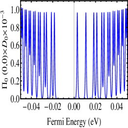
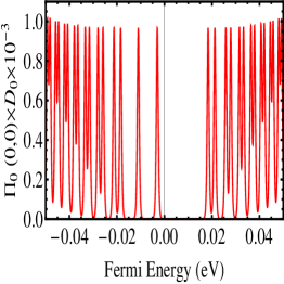
Figure 1: Static density-density correlation function in the long-wavelength limit $q\to 0$ versus Fermi energy $E_{F}$. We vary the field $E_{z}$ and the SOC strength $\lambda$. Left panel: the dashed and solid a curves are for $V=\lambda=0$ and $V=0$ meV and $\lambda=4$ meV. The other two panels are for $V=7$ meV and $\lambda=4$ meV; the middle panel is for the $K$ valley and the the right one for the $K^{\prime}$ valley. The degeneracy of the LLs is lifted.

We show numerical results of Eq. (16) as a function of the Fermi energy in Fig. 1. We find that the $n=0$ LL is split into four levels and all other LLs ($n>0$) into two. The valley degeneracy is lifted by the application of the field $E_{z}$ and the spin degeneracy by the SOC. This is consistent with the eigenvalues given by Eq. (2). We use $B$ = 1 Tesla, $T=3$ K, and vary the field energy $V=2lE_{z}$ and the SOC strength. The left panel is drawn for $V=\lambda=0$ (dashed curves) and $V=0$ meV and $\lambda=4$ meV ( solid curves). The other two panels are for $V=7$ meV and $\lambda=4$ meV; the middle panel is for the $K$ valley and the the right one for the $K^{\prime}$ valley.

In Fig. 1 the SOC and field split the LLs in two groups: in accordance with Eq. (2), $\eta,s={\pm}$, we label them as $+\equiv+,+\equiv-,-$ and $-\equiv-,+\equiv+,-$. Every $n\neq 0$ LL is doubly degenerate in each group and consists of a spin-up state from one valley and a spin-down state from the other valley. The LL splitting between the two groups is symmetric in the valence and conduction band due to the symmetry in Eq. (2). The four-fold spin and valley degeneracy of the $n=0$ LL is lifted by the SOC and electric field energy.

iii) zero frequency. The static limit $\omega\rightarrow 0$ of Eq. (6) is obtained with the help of Eqs. (7)-(8). In this limit $\operatorname{Im}\Pi_{0}(q,\omega)\rightarrow 0$ and Eq. (6) gives

$$\Pi_{0}(q,0)=\frac{1}{D_{0}}\sum_{n,n^{\prime}}\frac{f(E_{n}^{\eta,s})-f(E_{n^{\prime}}^{\eta,s})}{E_{n}^{\eta,s}-E_{n^{\prime}}^{\eta,s}}\,J_{nn^{\prime}}(u).$$ (17)

We show numerical results for $\Pi_{0}(q,0)$ as a function of the wave vector $q$ in Fig. 2. We use the parameters $B$ = 5 Tesla, $T$ = 10 K, and vary the field energy $V=2lE_{z}$ and the SOC strength $\lambda$. The black curves are for $V=\lambda=0$, the red ones for $V=0$ meV and $\lambda=4$ meV, and the blue curves for $V=10$ meV and $\lambda=4$ meV. The solid and dashed curves pertain, respectively, to spin up and $K$ valley and to spin down and $K^{\prime}$ valley.

In the usual 2DEG the screening wave vector is independent of the carrier density but for graphene or silicene it is proportional to the square root of the density 16 . First, in the limit of zero magnetic field $B$ the static correlation function remains constant and equal to the electronic density of states up to the wave vector of $q=2k_{F}$; there are two contributions to it that stem from intraband and interband plasmons, respectively. In the large momentum transfer regime of Fig. 2, $q\sim 5$ ($10^{8}$ m^-1, the static screening for the intraband case decreases linearly with $q$, which is consistent with the case of gapless graphene in the limit of zero (see Fig. 2 of Ref. 16 and Fig. 4 of Ref. 31 ) and finite 23 magnetic field. There is no possibility of zero-energy plasmon excitations in the intraband region (valence or conduction band).

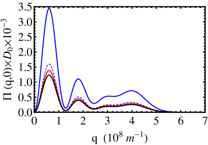
Figure 2: Static density-density correlation function versus the wave vector $q$. We vary the electric field energy $V$ and the SOC strength $\lambda$. Black curves: $V=\lambda=0$; red curves $V=0$ meV, $\lambda=4$ meV; blue curves $V=10$ meV and $\lambda=4$ meV. The solid and dashed curves pertain, respectively, to spin up and spin down in the $K$ valley or spin down and spin up in the $K^{\prime}$ valley. Here we cannot distinguish between the black (or red) solid and dashed curves as there is no spin or valley splitting for the chosen parameters.

We find a similar behaviour for finite $B$ except in the small wave vector limit. In contrast with its behaviour at $B=0$, the static correlation function tends to zero as $\Pi_{0}(q\rightarrow 0,0)\propto q^{2}$ for finite $B$ 23 . This is due to the fact that the main contribution to it comes from the $q=0$ excitations in the vicinity of $E_{F}$. Whereas at $B=0$ there are $q\to 0$ excitations whose energy tends to zero, $E_{F}$ now lies in a cyclotron gap between the highest occupied landau level $n_{F}$ and lowest unoccupied $n_{F}+1$. This gap must be overcome by small-$q$ excitations, such that its spectral weight approaches zero. The static correlation function also coincides with the density of states at $E_{F}$ because the latter vanishes for finite fields $B$ when $E_{F}$ is in the gap. Further, the oscillatory behaviour of the static correlation function below $2k_{F}$ is due to intraband transitions, whether $E_{F}$ is in the valence or conduction band ($n_{F}+1,n_{F}$).

IV Magnetoplasmons

Magnetoplasmons are readily furnished by the singularities of the function $\Pi_{1}(q,\omega)$, from the roots of the longitudinal magnetoplasmon dispersion relation obtained from Eq. (9) as

$$1-v_{c}(q)\Pi_{1}(q,\omega)=0,$$ (18)

along with the condition $\Pi_{2}(q,\omega)=0$ to ensure long-lived excitations 22 ; 23 ; 29 ; 30 , which is in excellent agreement with high-mobility graphene samples 28 .

For weak damping the decay rate $\gamma$, determined by Eqs. (10) and (12), is given by Eq. (22) of Ref. 30 . Since we are primarily interested in the long-wavelength behavior of undamped magnetoplasmons, described by $\gamma\propto\Pi_{2}(q,\omega)=0$, we treat them by solving Eq. (18). With the help of Eq. (10) we find its roots are obtained by solving

$$1=\frac{e^{2}}{kql^{2}}\underset{n,n^{\prime}}{\sum}J_{nn^{\prime}}(u)\big{[}I_{1}(\omega)+I_{1}(-\omega)\big{]}.$$ (19)

Using Eq. (11) we can write

$$I_{1}(\omega)+I_{1}(-\omega)=\frac{2\Delta_{n,n^{\prime}}^{\eta,s}}{\hbar^{2}\omega^{2}-(\Delta_{n,n^{\prime}}^{\eta,s})^{2}}\,f(E_{n}^{\eta,s}),$$ (20)

where $\Delta_{n,n^{\prime}}^{\eta,s}=E_{n^{\prime}}^{\eta,s}-E_{n}^{\eta,s}$. Next we expand $J_{nn^{\prime}}(u)$ to lowest order in its argument (low wave-number expansion). This amounts to considering only the $n^{\prime}=n\pm 1$ terms in Eq. (19). The inter-Landau level plasmon modes under consideration arise from neighbouring Landau levels, that is, from $n^{\prime}=n\pm 1$. Then using the expansion 33 $L_{n}^{{}^{l}}(u)={\displaystyle\sum\limits_{m=0}^{n}}\frac{(-1)^{m}\,(n+l)!}{(l+m)!(n-m)!}\frac{u^{m}}{m!}$ for $l>0$ and retaining only terms that are constant or linear in $u$ we get

$$J_{n,n+1}(u)\rightarrow nuG^{C}+(n+1)uG^{D},$$ (21)

$$J_{n,n-1}(u)\rightarrow(n-1)uG^{C}+nuG^{D}.$$ (22)

Here $G^{C}=(1+r_{\xi})/2$, $G^{D}=(1-r_{\xi})/2$, and $r_{\xi}=V_{\xi}/[\hslash^{2}\omega_{c}^{2}n+V_{\xi}^{2}]^{1/2}$. The factors $G^{C}$ and $G^{D}$ arise from the normalization of the eigenstates and in the limit $\lambda=E_{z}=0$ are both equal to 1/2.

To obtain the magnetoplasmon spectrum, we evaluate $\Delta_{n,n^{\prime}}^{\eta s}$ for $n^{\prime}=n\pm 1$. We find

$$\Delta_{n,n\pm 1}^{\eta,s}=\pm\,\hbar\omega_{c}/(2\big{[}n+(V_{\xi}/\hbar\omega_{c})^{2}\big{]}^{1/2}).$$ (23)

Substitution of Eqs (20)-(22) into Eq. (19) yields

$$1=\frac{e^{2}q}{\kappa}\sum_{n}\,\frac{|\Delta_{n,n\pm 1}^{\eta,s}|}{\hslash^{2}\omega^{2}-\big{(}\Delta_{n,n\pm 1}^{\eta,s}\big{)}^{2}}\,f(E_{n}^{\eta,s}).$$ (24)

For inter-LL excitations near the Fermi energy $E_{F}$ we can approximate $n$ by $n_{F}$ in $\Delta_{n,n\pm 1}^{\eta,s}$, where $n_{F}$ is the LL index corresponding to $E_{F}$. This gives

$$\hslash^{2}\omega^{2} =(\hbar^{2}\omega_{c}^{2}/(4\big{[}n_{F}+(V_{\xi}/\hbar\omega_{c})^{2}\big{]}))$$ (25)

$$\times\Big{[}1+\frac{2e^{2}q\big{[}n_{F}+(V_{\xi}/\hbar\omega_{c})^{2}\big{]}^{1/2}}{\kappa\hbar\omega_{c}}\,\sum_{n}f(E_{n}^{\eta,s})\Big{]}.$$

With $E_{F}$ in the conduction band ($E_{F}^{2}=\hslash^{2}\omega_{c}^{2}n_{F}+V_{\xi}^{2}$) Eq. (25) can be expressed as

$$\omega^{2}=\tilde{\omega}_{c}^{2}+\tilde{\omega}_{p}^{2},$$ (26)

where

$$\tilde{\omega}_{c}=\omega_{c}\big{[}\hbar\omega_{c}/(2(\hbar^{2}\omega_{c}^{2}n_{F}+V_{\xi}^{2})^{1/2})\big{]},$$ (27)

and

$$\tilde{\omega}_{p}=\omega_{p}\big{[}v_{F}/(\hbar^{2}\omega_{c}^{2}n_{F}+V_{\xi}^{2})^{1/4}\big{]},$$ (28)

with $\omega_{p}=\big{[}e^{2}q\pi n_{c}/\kappa\big{]}^{1/2}$ and $n_{c}=\underset{n}{\sum}f(E_{n}^{\eta,s})/(\pi\ell^{2})$ the 2D carrier density.

It is interesting that Eq. (24) can be applied to the usual 2DEG for which $\Delta_{n,n\pm 1}^{\eta,s}=\pm\hslash\omega_{c}$. Then we obtain again Eq. (26) with $\tilde{\omega}_{c}$ and $\tilde{\omega}_{p}$ replaced, respectively, by $\omega_{c}=eB/m$ and $\omega_{p}=\big{[}e^{2}q\pi n_{c}/\kappa\big{]}^{1/2}$, that is, the well-known plasmon dispersion relation. One can also take the limit $V_{\xi}\to 0$ in Eqs. (24)-(28) and obtain the dispersion relation for monolayer graphene 23 ; 28 . Then $\Delta_{n,n\pm 1}^{\eta,s}=\pm\hslash\omega_{c}/(2n^{1/2})$, $\tilde{\omega}_{c}=\omega_{c}/(2\sqrt{n_{F}})$, and $\tilde{\omega}_{p}=(v_{F}/(2n_{F}^{1/4}\sqrt{\hslash\omega_{c}}))\,\omega_{p}.$

In the limit of zero magnetic field, Eqs. (26)-(28) reduce to recent work on silicene and germanene 29 ; 30 . Moreover, in the limit of zero SOC and $E_{z}$, these relations are the same as that for high-mobility graphene samples 28 and could be applied to highly doped graphene samples 26 ; 27 (for very large $n_{F}$ in Eq. (25). The $q$ dependence of Eq. (26), namely the $\sqrt{q}$ behaviour, is common to 2D electron gas systems while the carrier density dependence is characteristic of the linear-in-$k$ dispersion relation of massless Dirac fermions, for which $E_{F}=\hslash v\sqrt{\pi n_{c}}$. However, in the present case we can see the effects of gapped silicene or germanene with massive Dirac fermions and spin/valley splitting due to the combination of the SOC and the electric field $E_{z}$.

V Discussion of results

A closer analytical examination of Eq. (26) shows the following aspects of the gapped magnetoplasmon spectrum. If we set $E_{z}=0$ in Eq. (26) we obtain a SOC-induced, small-gap magnetoplasmon spectrum. Increasing $E_{z}$, we obtain a larger gap, splitting and tuning of plasmons in silicene by combining it with the SOC. If we use a field $E_{z}$ comparable to the SOC strength $\lambda$, then we expect splitting of the magnetoplasmon modes due to the combination of the two in the quantity $V+\eta s\lambda$. With further increase in $E_{z}$ , e.g., $E_{z}=2\lambda$  we can see an enhanced spin and valley splitting of the magnetoplasmon spectrum due to the $V+\eta s\lambda$ factor in Eq. (21). Moreover, we note that the realization of topological phase transitions could also be observed in the magnetoplasmon spectrum if we take $E_{z}$ zero or less than $\lambda$ (spin-Hall regime), comparable to $\lambda$ (semi-metallic regime), and then twice $\lambda$ (valley-Hall regime). The spin-Hall regime is a topological insulator while the valley-Hall one is a band insulator. For $B\to 0$ these transitions are consistent with recent plasmon predictions 29 ; 30 . Below we consider the effect of an external field $B$ using the parameters 7 ; 26 ; 27 ; 28 ; 29 ; 30 : $q=\pi/100$ nm^-1, $v_{F}=0.5\times 10^{6}$ m/s, $\lambda=4$ meV for silicene ($43$ meV for germanene) on SiC with dielectric constant $\kappa\simeq 4$ (different values do not qualitatively affect the results), and carrier density $n_{c}=0.5\times 10^{16}$ m^-2 giving $E_{F}=$ 41.3 meV.

The changes in the density of states $D(E)$ discussed in Sec. III and the approximations used to obtain the magnetoplasmons are reflected in the dependence of $E_{F}$, e.g., on the mangetic field. At finite temperatures the 2D carrier density $n_{c}$ is $n_{c}=\int_{-\infty}^{\infty}D(E)f(E)dE$, with $D(E)$ for the LL spectrum obtained as

$$D(E)=\frac{1}{D_{0}}\left(\frac{1}{2}\sum_{\eta,s}\delta(E-E_{0}^{\eta,s})+\sum_{n=1,\eta,s}\delta(E-E_{n}^{\eta,s})\right);$$ (29)

the factor $1/2$ refers the fact the degeneracy of the zero LL is half that of the other LLs. Using Eq. (29) the result for $n_{c}$ becomes

$$n_{c}=\frac{1}{D_{0}}\left(\frac{1}{2}\sum_{\eta,s}f(E_{0}^{\eta,s})+\sum_{n=1,\eta,s}f(E_{n}^{\eta,s})\right).$$ (30)

Figure 3: Fermi energy as a function of magnetic field for fixed values $V=10$ meV, $\lambda=4$ meV, and $n_{c}=0.5\times 10^{16}$ m^-2. The temperature is varied such that $T=10$ K (solid) and $T=5$ K (dotted).

For fixed carrier density, this determines $E_{F}$ implicitly by solving numerically Eq. (30). We show the resulting $E_{F}$, as a function of the magnetic field $B$ in Fig. 3, for $V=10$ meV, $\lambda=4$ meV, $T=10$ K, and $n_{c}=0.5\times 10^{16}$ m^-2. $E_{F}$ remains constant for low $B$ below 2T, that is, in the limit of large $n$; above this value we see the jumps as $E_{F}$ crosses the LLs.

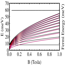
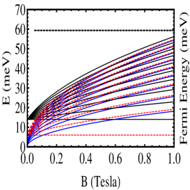
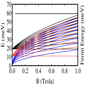
Figure 4: Band structure of silicene as a function of the magnetic field $B$. The blue curves correspond to $\lambda=V=0$ and the black and red dotted ones to $E_{n}^{+}$ and $E_{n}^{-}$, respectively. The black dotted line shows $E_{F}$ vs $B$ evaluated numerically using Eq. (30). In the left panel we cannot distinguish between the blue and red dotted curves because at $\lambda=V=$ 4 meV the gap is zero for the ($V-\lambda$) curves. In the middle panel we see a clear degree of spin and valley splitting for $\lambda=$ 4 meV and $V=$ 10 meV. The right panel, for $\lambda=$ 4 meV and $V=$ 15 meV, shows a significant degree of spin and valley splitting by electrical tuning.

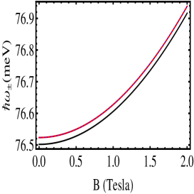
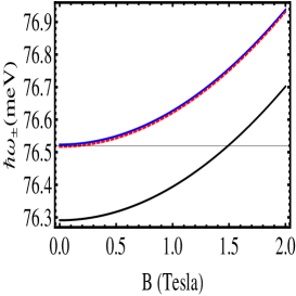
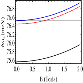
Figure 5: Magnetopasmons as a function of the magnetic field $B$ for a fixed $E_{F}=41.3$ meV. Blue curves correspond to $\lambda=V=0$.Black and red dotted curves represent $\hslash\omega_{+}$ and $\hslash\omega_{-}$, respectively. In the left panel, with $\lambda=V=$ 4 meV, we cannot distinguish between the red and blue dotted curves because at equal amount of $V$ and $\lambda$ energies, the gap is zero for the ($V-\lambda$) curves. The middle panel, for $\lambda=$ 4 meV and $V=$ 10 meV, shows a clear signature of spin and valley splitting. The right panel, for $\lambda=$ 4 meV and $V=$ 15 meV, shows a significant spin and valley splitting by electrical tuning. The colour code is the same as in Fig. 4.

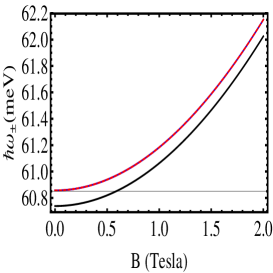
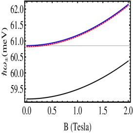
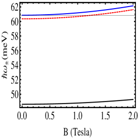
Figure 6: Magnetopasmons as a function of the magnetic field $B$ for a fixed $E_{F}=26$ meV. The parameters and curve marking are the same as in Fig. 5.

We present the eigenvalues given by Eq. (2) as a function of the field $B$ for fixed values of $\lambda$ and $E_{z}$ in Fig. 4. We also include the $E_{F}$ versus field $B$ curve (dotted line) for comparison and further discussion. We find the following: (i) In the limit of $\lambda=\ell E_{z}=0$ (blue curves), we obtain the $\sqrt{B}$ dependence of the LL energies. In contrast, for finite $\lambda$ and variable $E_{z}$ (black and red dotted curves), the energies of the lower LLs grow linearly with $B$ rather than with $\sqrt{B}$ because of the massive Dirac fermions in silicene or germanene. (ii) The combination of the field energy $V=2\ell E_{z}$ and $\lambda$ splits the LLs in two groups designated as $E_{n}^{\pm}$, with $E_{n}^{+}\equiv E_{n}^{+,+}=E_{n}^{-,-}$ and $E_{n}^{-}\equiv E_{n}^{-,+}=E_{n}^{+,-}$. (iii) The energies of the two groups of LLs in the valence or conduction band have not only different slopes versus $B$ but also shift rigidly for $B\to 0$ due to the finite band gap either by $\lambda$ or by the field $E_{z}$. However, every $n\neq 0$ LL is still doubly degenerate in each group, consisting of a spin-up state from one valley and a spin-down state from the other valley. A crossing occurs between the two groups, which is symmetric in the valence and conduction band due to the symmetry in Eq. (2).

In Fig. 5 we show the magnetoplasmon spectrum as a function of the field $B$ for fixed $E_{F}$ = 41.3 meV. For comparison with graphene experiments 28 , we show numerical results using Eq. (26) for $\lambda=V=0$ (blue curve). These results agree well with Eq. (1) and Fig. 2 of Ref. 28 , exhibiting dependence on $\sqrt{B}$, if we replace $v_{F}=0.5\times 10^{6}$ m/s by its value in graphene $v_{F}=1\times 10^{6}$ m/s. In the middle panel, for finite $\lambda$ and $V=2lE_{z}$, we found two curves, the red dotted ($V-\lambda$) and black ($V+\lambda$) showing a spin and valley splitting. The red dotted curve is the same as the blue one and we can’t distinguish between the two because the gap for the red dotted line vanishes due to $\lambda-2lE_{z}=0$. As the gap due to $\lambda$ and $V$ is small and we are in a highly doped regime, we can see a split between the red dotted and black curve for two magnetoplamon modes $\hslash\omega_{\pm}$ defined as $\hslash\omega_{+}=\hslash\omega_{+,+}=\hslash\omega_{-,-}$ and $\hslash\omega_{-}=\hslash\omega_{-,+}=\hslash\omega_{+,-}$. Increasing $V=2lE_{z}=10$ meV, we see an enhanced splitting between red dotted and black curves for fixed $\lambda=4$ meV (middle panel). Here the blue and red dotted curves are weakly separated as the gap vanishes for the blue and red dotted curves $V-\lambda=6$ meV. With further increase in $V$, $V=15$ meV, we obtain a further enhanced splitting between the black and red dotted curves of the magnetoplasmon modes as shown in the right panel for fixed $\lambda=4$ meV. We also note that the blue and red dotted lines are well separated as gap is zero for the blue and $V-\lambda=$ 11 meV for the red dotted curve.

We contrast our results with those of recent graphene experiments on high-mobility or weakly doped samples 28 , in the limit $\lambda=2\ell E_{z}=0$, by further decreasing the Fermi energy close to the Dirac point. First, we show the magnetoplasmon spectrum as a function of the field $B$ for $E_{F}=26$ meV in Fig. 6. We found a clear splitting between the black and red dotted curves for $\lambda=2lE_{z}=4$ meV (left panel) as in the left panel of Fig. 5. As $\lambda$ and $E_{z}$ are small and we are in a weakly doped regime, we can see a strong splitting for the magnetoplamon modes $\hslash\omega_{\pm}$. Again here we cannot distinguish between the red dotted and blue curves for the same reason as in Fig. 5. Upon increasing $V$, e.g. to $V=10$ meV, we see a large splitting between the red dotted and black curves for fixed $\lambda=4$ meV (middle panel). We can weakly distinguish between the blue and red dotted curves here since the gap is $V-\lambda=6$ meV for the red dotted curve and zero for the blue one. With further increase in $V$, $V=15$ meV, we obtain a significant splitting between the red dotted and black curves of the magnetoplasmon modes as shown in the right panel. Here we also note that the blue and red dotted curves are well separated compared to those in the right panel of the Fig. 5. Again the results exhibit a square-root dependence on B and agree with recent graphene theory 21 ; 22 ; 23 ; 24 ; 25 and experiments 28 in the limit $\lambda=2\ell E_{z}=0$ provided we use $v_{F}=1\times 10^{6}$ m/s.

The experimentally observed 28 , $\sqrt{B}$ dependence of the spectrum referred to above, in the limit $\lambda=V\to 0$, applies to high-mobility weakly-doped graphene samples, cf. Fig. 6. For highly-doped samples 26 ; 27 though that involve values of $E_{F}\gg\lambda,V$, with $E_{F}$ of the order of $200-300$ meV, the magnetoplasmon gaps and spilttitings reported above will be very difficult to achieve as they would require unrealistically high values of $V$. Notice though that our analysis for silicene also holds for germanene, a monolayer of germanium, which has a much stronger SOC than silicene 7 ; 8 , $\lambda\approx 43$ meV. In both cases the predicted gaps and spilttings are sizeable for $E_{F}$ not too far from the Dirac point.

Another feature of our results is the magnetoplasmon gaps. Although not yet experimentally confirmed, the SOC induced gap in silicene is about 1.55 meV [6,7] and is expected to be observed using existing experimental techniques. In the present work on electrically tunable magnetoplasmons in silicene, we have obtained a gap of about 1 meV in Fig. 5 and 12 meV in Fig. 6 tuned by an external perpendicular electric field, which can be further enhanced by increasing this electric field and lowering the Fermi energy of the system close to the Dirac point. We believe that this gap can be observed in experiments similar to those on high-mobility graphene samples studying magnetoplasmons [28].

A possible extension of our work would be to include an in-plane electric field and study magneto-electric-plasmons. One could then use the eigenfunctions and eigenvalues derived in Ref. per for $E_{z}=\lambda=0$ as a starting point.

VI Summary

We showed electrically tunable effects in the magnetoplasmon spectrum of silicene and germanene due to the spin and valley polarization. Employing the RPA and including the effects of SOC and of an external electric field, we found a significant splitting of the magnetoplasmon spectrum. Our results agree well with graphene theory and experiments in the limit of vanishing SOC and electric field provided $E_{F}$ is not too far from the Dirac point, that is, for weakly-doped graphene samples 28 , if we use graphene’s value for $v_{F}$. We expect that experimental studies of these novel phenomena in silicene, similar to those of Ref. [28], will be very appropriate since they directly bear on the many-body properties of silicene or germanene. Encouraging in this direction is the very recently reported local formation of high-buckled silicene nanosheets realized on a MoS₂ surface [35].

Electronic address: ^†m.tahir06@alumni.imperial.ac.uk

Appendix A

Below we outline the derivation of Eq. (8). The factor $J_{\alpha,\alpha^{\prime}}(u)$ in Eq. (7) is given by

$$J_{\alpha,\alpha^{\prime}}(u)=\left\langle\alpha^{\prime}\right|\left|e^{-i\mathbf{q\cdot r}}\right|\left|\alpha\right\rangle^{2}=\left\langle\alpha^{\prime}\right|\left|e^{-i\mathbf{q\cdot r}}\right|\left|\alpha\right\rangle\times\left\langle\alpha\right|\left|e^{i\mathbf{q\cdot r}}\right|\left|\alpha^{\prime}\right\rangle,$$ (A.1)

where $\left|\alpha\right\rangle=\left|s,n,\eta,k_{y}\right\rangle$. Using the eigenfunctions given by Eq. (3) Eq. (A.1) takes the form

$$\left\langle\alpha^{\prime}\right|\left|e^{-i\mathbf{q\cdot r}}\right|\left|\alpha\right\rangle=\frac{1}{L_{y}}\sum_{n,\eta,s}{\displaystyle\int}dye^{i\left(k_{y}-k_{y}^{\prime}-q_{y}\right)y}{\displaystyle\int\limits_{-\infty}^{\infty}}dx\left(\begin{array}[c]{c}-iC_{n}^{\eta,s}\phi_{n-1}(\bar{x})\\ D_{n}^{\eta,s}\phi_{n}(\bar{x})\end{array}\right)^{T}e^{-iq_{x}x}\left(\begin{array}[c]{c}-iC_{n}^{\eta,s}\phi_{n-1}(\bar{x})\\ D_{n}^{\eta,s}\phi_{n}(\bar{x})\end{array}\right),$$ (A.2)

where the superscript $T$ denotes the transpose of the column vector. With the help of the identity $(1/L_{y})\int dy\,e^{i\left(k_{y}-k_{y}^{\prime}-q_{y}\right)y}=\delta_{k_{y}^{\prime},k_{y}-q_{{}_{y}}}$ we can write Eq. (A.2) as

$$\left\langle\alpha^{\prime}\right|\left|e^{-i\mathbf{q\cdot r}}\right|\left|\alpha\right\rangle=\delta_{k_{y}^{\prime},k_{y}-q_{{}_{y}}}\sum_{n,\eta,s}\Big{[}F_{n^{\prime},n}\left(-q_{x},k_{y}-q_{y},k_{y}\right)+F_{n^{\prime}-1,n-1}\left(-q_{x},k_{y}-q_{y},k_{y}\right)\Big{]}.$$ (A.3)

Similarly,

$$\left\langle\alpha\right|\left|e^{i\mathbf{q\cdot r}}\right|\left|\alpha^{\prime}\right\rangle=\delta_{k_{y}^{\prime},k_{y}-q_{{}_{y}}}\sum_{n,\eta,s}\Big{[}F_{n,n^{\prime}}\left(q_{x},k_{y},k_{y}-q_{y}\right)+F_{n-1,n^{\prime}-1}\left(q_{x},k_{y},k_{y}-q_{y}\right)\Big{]}.$$ (A.4)

Combining Eqs. (A.3) and (A.4), we arrive at

$$J_{n,n^{\prime}}(u) =\delta_{k_{y}^{\prime},k_{y}-q_{{}_{y}}}\sum_{n,\eta,s}\Big{[}F_{n^{\prime},n}\left(-q_{x},k_{y}-q_{y},k_{y}\right)\times F_{n,n^{\prime}}\left(q_{x},k_{y},k_{y}-q_{y}\right)$$

$$\hskip 65.44142pt+F_{n^{\prime}-1,n-1}\left(-q_{x},k_{y}-q_{y},k_{y}\right)\times F_{n-1,n^{\prime}-1}\left(q_{x},k_{y},k_{y}-q_{y}\right)\Big{]}.$$ (A.5)

Now we proceed with the evaluation of $F_{n^{\prime}n}\left(-q_{x},k_{y}-q_{y},k_{y}\right)$. Using the explicit form of the harmonic oscillator functions $\phi_{n}(\bar{x})$ we have

$$F_{n^{\prime}n}\left(-q_{x},k_{y}-q_{y},k_{y}\right)=\frac{[D_{n^{\prime}}^{\eta,s}D_{n}^{\eta,s}]}{l^{2}\sqrt{\pi 2^{n}2^{n^{\prime}}n!n^{\prime}!}}{\displaystyle\int\limits_{-\infty}^{\infty}}dX\text{ }e^{-\left(X+l\left(k_{y}-q_{y}\right)\right)^{2}/2}$$

$$\hskip 110.96556pt\times H_{n^{\prime}}\left(X+l\left(k_{y}-q_{y}\right)\right)e^{-iq_{x}x}\,e^{-\left(X+lk_{y}\right)^{2}/2}\,H_{n}\left(X+lk_{y}\right),$$ (A.6)

where $X=x/l$. Making the change $Y=X+lk_{y}+l\left(-q_{y}+iq_{x}\right)/2$ in Eq. (A.6) yields

$$F_{n^{\prime}n}\left(-q_{x},k_{y}-q_{y},k_{y}\right) {\small=}\frac{[D_{n^{\prime}}^{\eta,s}D_{n}^{\eta,s}]}{\sqrt{\pi 2^{n}2^{n^{\prime}}n!n^{\prime}!}}\,e^{-u^{2}}e^{il^{2}q_{x}\left(-q_{y}+2k_{y}\right)/2}$$

$$\times{\displaystyle\int\limits_{-\infty}^{\infty}}dY\,e^{-Y^{2}}H_{n^{\prime}}\left(Y-l\left(q_{y}+iq_{x}\right)/2\right)H_{n}\left(Y-l\left(q_{y}-iq_{x}\right)/2\right),$$ (A.7)

where $u=l^{2}{q}^{2}/2$. The integral over $Y$ is tabulated in Ref. 34, pp. 838 #7.377. The result for $n\leq n^{\prime}$ is

$$F_{n^{\prime}n}\left(-q_{x},k_{y}-q_{y},k_{y}\right) =\left(n!/n^{\prime}!\right)^{1/2}e^{-u/2+il^{2}q_{x}\left(-q_{y}+2k_{y}\right)/2}$$

$$\times\left[l\left(q_{y}-iq_{x}\right)/\sqrt{2}\right]^{n^{\prime}-n}L_{n}^{n^{\prime}-n}\left(u\right).$$ (A.8)

For $n^{\prime}\leq n$, the result is given by Eq. (A.8) with $n$ and $n^{\prime}$ interchanged. Using Eqs. (A.5) and (A.8) we arrive at Eq. (7),

$$J_{n,n^{\prime}}(u)=\ \left|\left\langle\alpha^{\prime}\right|e^{-i\mathbf{q\cdot r}}\left|\alpha\right\rangle\right|^{2}=\delta_{k_{y}^{\prime},k_{y}-q_{{}_{y}}}\Big{\{}[D_{n^{\prime}}^{\eta,s}D_{n}^{\eta,s}]F_{nn^{\prime}}\left(u\right)+[C_{n^{\prime}}^{\eta,s}C_{n}^{\eta,s}]F_{{}^{n-1,n^{\prime}-1}}\left(u\right)\Big{\}}^{2},$$ (A.9)

with $F_{nn^{\prime}}\left(u\right)$ given after Eq. (7) in the text.

References

- (1) K. S. Novoselov, A. K. Geim, S. Morozov, D. Jiang, Y. Zhang, S. Dubonos, I. Grigorieva, and A. A. Firsov, Science 306, 666 (2004).
- (2) A. H. Castro Neto, F. Guinea, N. M. R. Peres, K. S. Novoselov, and A. K. Geim, Rev. Mod. Phys. 81, 109 (2009).
- (3) G. G. Guzmán-Verri and L. C. Lew Yan Voon, Phys. Rev. B 76, 075131 (2007); S. Lebègue and O. Eriksson, Phys. Rev. B 79, 115409 (2009).
- (4) P. Vogt, P. D. Padova, C. Quaresima, J. Avila, E. Frantzeskakis, M. C. Asensio, A. Resta, B. Ealet, and G. L. Lay, Phys. Rev. Lett. 108, 155501 (2012); A. Fleurence, R. Friedlein, T. Ozaki, H. Kawai, Y. Wang, and Y. Yamada-Takamura, ibid. 108, 245501 (2012).
- (5) C. L. Lin, R. Arafune, K. Kawahara, M. Kanno, N. Tukahara, E. Minamitani, Y. Kim, M. Kawai, N. Takagi, Phys. Rev. Lett. 110, 076801 (2013); Z. X. Guo, S. Furuya, J. Iwata, A. Oshiyama, J. Phys. Soc. Jpn. 82, 063714 ( 2013); Y. P. Wang, H. P. Cheng, Phys. Rev. B 87, 245430 (2013).
- (6) C.-C Liu , W. Feng, and Y. Yao, Phys. Rev. Lett. 107, 076802 (2011).
- (7) C.-C. Liu, H. Jiang, and Y. Yao, Phys. Rev. B 84, 195430 (2011).
- (8) M. Ezawa, Phys. Rev. Lett. 109, 055502 (2012); New J. Phys. 14, 033003 (2012).
- (9) Y. Cai, C.-P. Chuu, C. M. Wei, and M. Y. Chou, Phys. Rev. B 88, 245408 (2013).
- (10) H. Liu, J. Gao, and J. Zhao, J. Phys. Chem. C, 117, 10353 (2013).
- (11) M. Neek-Amal, A. Sadeghi, G. R. Berdiyorov, and F. M. Peeters, Appl. Phys. Lett. 103, 261904 (2013).
- (12) M. Tahir, A. Manchon, K. Sabeeh, and U. Schwingenschlögl, Appl. Phys. Lett. 102, 162412 (2013).
- (13) C. J. Tabert and E. J. Nicol, Phys. Rev. B 87, 235426 (2013).
- (14) M. Tahir and U. Schwingenschlögl, Sci. Rep. 3, 1075 (2013).
- (15) C. J. Tabert and E. J. Nicol, Phys. Rev. Lett. 110, 197402 (2013).
- (16) E. H. Hwang and S. D. Sarma, Phys. Rev. B 75, 205418 (2007); X.-F. Wang and T. Chakraborty, Phys. Rev. B 75, 033408 (2007).
- (17) L. Ju, B. Geng, J. Horng, C. Girit, M. Martin, Z. Hao, H. A. Bechtel, X. Liang, A. Zettl, Y. R. Shen, and F. Wang, Nat. Nanotechnol. 6, 630 (2011).
- (18) V. N. Kotov, B. Uchoa, V.M. Pereira, F. Guinea, and A. H. Castro Neto, Rev. Mod. Phys. 84, 1067 (2012).
- (19) Z. Fei, A. S. Rodin, G. O. Andreev, W. Bao, A. S. McLeod, M. Wagner, L.M. Zhang, Z. Zhao, M. Thiemens, G. Dominguez, M. M. Fogler, C. A. H. Neto, C. N. Lau, F. Keilmann, and D. N. Basov, Nature (London) 487, 82 (2012).
- (20) J. Chen, M. Badioli, P. Alonso-Gonzalez, S. Thongrattanasiri, F. Huth, J. Osmond, M. Spasenovic, A. Centeno, A. Pesquera, P. Godignon, E. A. Zurutuza, N. Camara, F. J. G. de Abajo, R. Hillenbrand, and F. H. L. Koppens, Nature (London) 487, 77 (2012).
- (21) M. Tahir and K. Sabeeh, J. Phys.: Condens. Matter 20, 425202 (2008).
- (22) R. Roldan, M. O. Goerbig, and J. -N. Fuchs, Phys. Rev. B 83, 205406 (2011).
- (23) M. O. Goerbig, Rev. Mod. Phys. 83, 1193 (2011).
- (24) J. Y. Wu, S. C. Chen, O. Roslyak, G. Gumbs, and M. F. Lin, ACS Nano 5, 1026 (2011).
- (25) M. Tymchenko, A. Y. Nikitin, and L. M. Moreno, ACS Nano 7, 9780 (2013).
- (26) I. Crassee, M. Orlita, M. Potemski, A. L. Walter, M. Ostler, Th. Seyller, I. Gaponenko, J. Chen, and A. B. Kuzmenko, Nano Lett. 12, 2470 (2012).
- (27) H. G. Yan, Z. Li, X. Li, W. Zhu, P. Avouris, and F. Xia, Nano Lett. 12, 3766 (2012).
- (28) J. M. Poumirol, W. Yu, X. Chen, C. Berger, W. A. de Heer, M. L. Smith, T. Ohta, W. Pan, M. O. Goerbig, D. Smirnov, and Z. Jiang. Phys. Rev. Lett. 110, 246803 (2013).
- (29) H. R. Chang, J. Zhou, H. Zhang, and Y. Yao, Phys. Rev. B 89, 201411 (2014).
- (30) C. J. Tabert, E. J. Nicol, Phys. Rev. B 89, 195410 (2014).
- (31) B. Van Duppen, P. Vasilopoulos, and F. M. Peeters, Phys. Rev. B 90, 035142 (2014).
- (32) T. Ando, J. Phys. Soc. Jpn. 75, 074716 (2006).
- (33) P. K. Pyatkovskiy and V. P. Gusynin, Phys. Rev. B 83, 075422 (2011).
- (34) I. S. Gradshteyn and I. M. Ryzhik, Tables of Integrals, Series and Products (Academic Press, New York), 1980.
- (35) D. Chiappe, E. Scalise, E. Cinquanta, C. Grazianetti, B. v. Broek, M. Fanciulli, M. Houssa, and A. Molle, Adv. Mater. 26, 2096 (2014).
- (36) N. M. R. Peres and E. V. Castro, J. Phys.: Condens. Matter 19 406231 (2007); Lukose V, Shankar R and Baskaran G, Phys. Rev. Lett. 98 116802 (2007); Phys. Rev. Lett. 98 116802; P. Krstajić and P. Vasilopoulos, Phys. Rev. B 83 075427 (2011).