Low-rank Approximation of Tensors via Sparse Optimization
Abstract
The goal of this paper is to find a low-rank approximation for a given tensor. Specifically, we give a computable strategy on calculating the rank of a given tensor, based on approximating the solution to an NP-hard problem. In this paper, we formulate a sparse optimization problem via an -regularization to find a low-rank approximation of tensors. To solve this sparse optimization problem, we propose a rescaling algorithm of the proximal alternating minimization and study the theoretical convergence of this algorithm. Furthermore, we discuss the probabilistic consistency of the sparsity result and suggest a way to choose the regularization parameter for practical computation. In the simulation experiments, the performance of our algorithm supports that our method provides an efficient estimate on the number of rank-one tensor components in a given tensor. Moreover, this algorithm is also applied to surveillance videos for low-rank approximation.
keywords:
-regularization, low-rank approximation, proximal alternating minimization, sparsityAMS:
15A69, 65F30siscsiscxxxx–x
1 Introduction
We have seen the success of the matrix SVD for several decades. However in the advent of modern and massive datasets, even SVD has its limitation. Since tensors have been known to be a natural representation of higher-order and hierarchical dimensional datasets, we focus on the extension of low rank matrix approximation to tensors. Tensors have received much attention in recent years in the areas of signal processing [11, 37, 38], computer vision [20, 30, 35, 42], neuroscience [2, 31], data science and machine learning [24, 42, 20, 1]. Most of these applications rely on decomposing a tensor data into its low-rank form to be able to perform efficient computing as well as to reduce memory requirements. This type of tensor decomposition into a sum of rank-one tensor terms is called the canonical polyadic (CP) decomposition; thus, it is viewed as a generalization of the matrix SVD. The generalization of matrix SVD to tensors is not unique. Another tensor decomposition is called the Higher-Order SVD [13, 24], which is a product of orthogonal matrices with a dense core tensor. Higher-order SVD is considered another extension of the matrix SVD.
Unlike the matrix case where the low-rank matrix approximation is afforded by truncating away small rank-one matrix terms [17], discarding negligible rank-one tensor terms does not necessarily provide the best low-rank tensor approximation [25]. Moreover, most low rank tensor algorithms do not provide an estimation on the tensor rank; an a priori tensor rank is often required to find the decomposition. Several theoretical results [26, 27] on tensor rank can help, but they are limited to low-multidimensional and low order tensors so they are inapplicable to tensors in real-life applications. In fact, for real dataset, tensor rank is important. In a source apportionment data problem [28], the tensor rank of the data provides the number of pollution source profiles to be identified. In this work, the focus is on finding an estimation of the tensor rank and its rank-one tensor decomposition (CP) of a given tensor. There are several numerical techniques [11, 15, 24, 33, 37] for approximating a th rank tensor into its CP decomposition, but they do not give an approximation of the minimum rank. There are algorithms [12, 5] which give tensor rank, but they are specific to symmetric tensor decomposition over the complex field using algebraic geometry tools.
Our proposed algorithm addresses two difficult problems for the CP decomposition: (a) one is that finding the rank of tensors is a NP-hard problem [21], and (b) the other is that tensors can be ill-posed [14] and failed to have their best low-rank approximations.
The tensor rank problem is formulated as an minimization problem; i.e.
| (1) |
where represents a sum of the outer products of the vectors and for . Here corresponds the number of nonzero coefficients in the sum. However, this problem formulation (1) is NP-hard. Inspired by the techniques in compressive sensing [7, 10, 18], we then consider an -regularization formulation for tensor rank,
| (2) |
Here we denote . It is well known in the compressed sensing community that minimizing the norm of the vector recovers the sparse solution of the linear system. In the presence of noise, the constraint, is replaced with where is the Frobenius norm with . Moreover, to achieve a tensor decomposition as well as tensor rank, we minimize over the factor matrices, and , thus this minimization problem is considered:
| (3) |
The -regularization achieves a good approximation of tensor rank due to the sparsity structure and its tractability. In addition, the -regularization term provides a restriction on the boundedness of the variables thereby ameliorating the ill-posedness of the best low-rank approximation of tensors. For more tractable computing, an alternative multi-block constraint optimization [4] is implemented, which is similar to the technique discussed in [42]. Since (3) is a minimization of a sum of a smooth term and a nonsmooth term, we consider the following optimization problem with smooth and non smooth terms:
| (4) |
where and are the smooth and nonsmooth functions, respectively. Here is approximated at a given point .
1.1 Contributions
Here we list our contributions in this paper:
- 1.
-
2.
We provide some theoretical results on the convergence of our algorithm. We show the objective function satisfies a descent property in Lemma 4 and a subdifferential lower bound [4]. A monotonically decreasing objective function is ensured on the sequence generated by the algorithm. Furthermore, we point out that the sequence generated by algorithm converges to a critical point of the objective function with indicator functions on the normalization constraint that all the columns of the factor matrices have length one.
-
3.
For practical implementation, we provide a technique (as well as theoretical results) to find a suitable choice on the regularization parameter directly from the data. The regularization parameter choice has remained a very challenging problem [34, 36, 23, 32] in applied inverse problems. Our technique is based on the probabilistic consistency of the sparsity in the classical model found in [41, 43]:
where is a sparse signal, is a design matrix and is a vector of independent subgaussian entries with mean zero and parameter . We show that to find the true sparsity structure with a high probability, the regularization parameter relies on two intrinsic parameters and of models, where represents the variance of noise, and is the incoherence parameter [41] on design matrix . The relationship between the regularization and intrinsic parameters actually provides us a suggestion on how to choose a reasonable regularization parameter for practical computation. To illustrate the performance of this low-rank approximation method, our experiment consists of four parts. In the first part, we show the relationship between the regularization parameter and the estimated rank. In the second part, we estimate the number of rank-one components for given tensors by adaptively selecting the regularization parameter . In the third one, we compare our algorithm with a modified alternating least-squares algorithm. In the last one, we handle the real surveillance video data.
1.2 Organization
Our paper is organized as follows. In Section 2, we provide some notations and terminologies used throughout this paper. In Section 3, we formulate an -regularization optimization to the low-rank approximation of tensors. In Section 4, we propose an algorithm to solve this -regularization optimization by using a rescaling version of the proximal alternating minimization technique. In Section 5 we discuss the probabilistic consistency of the sparse optimal solution and give a suggestion on how to choose the regularization parameter. The numerical experiments in Section 6 consist of simulated and real datasets. Finally, our conclusion and future work are given in Section 7.
2 Notation
We denote a vector by a bold lower-case letter . The bold upper-case letter represents a matrix and the symbol of tensor is a calligraphic letter . Throughout this paper, we focus on third-order tensors of three indices and , but all the methods proposed here can be also applied to tensors of arbitrary high order.
A third-order tensor has column, row and tube fibers, which are defined by fixing every index but one and denoted by , and respectively. Correspondingly, we can obtain three kinds and of matricization of according to respectively arranging the column, row, and tube fibers to be columns of matrices. We can also consider the vectorization for to obtain a row vector such the elements of are arranged according to varying faster than and varying faster than , i.e., .
The outer product of three nonzero vectors and is a rank-one tensor with elements for all the indices. A canonical polyadic (CP) decomposition of expresses as a sum of rank-one outer products:
| (5) |
where for . Every outer product is called as a rank-one component and the integer is the number of rank-one components in tensor . The minimal number such that the decomposition (5) holds is the rank of tensor , which is denoted by . For any tensor , has an upper bound [26].
The CP decomposition (5) can be also written as:
| (6) |
where is a rescaling coefficient of rank-one tensor for . For convenience, we let and in (6) where and are called the factor matrices of tensor . We impose a normalization constraint on factor matrices such that each column is normalized to length one [24, 39] which is denoted by . For most alternating optimization algorithms for tensors, flattening the tensor (matricization) is necessary to be able to break down the problem into several subproblems. Here we describe a standard approach for a matricizing of a tensor. The Khatri-Rao product of two matrices and is defined as
where the symbol “” denotes the Kronecker product:
Using the Khatri-Rao product, the decomposition (6) can be written in three different matrix forms of tensor [6]:
| (7) |
where the matrix is diagonal with elements of .
3 Sparse optimization for low-rank approximation
The main goal of this study is to find a tensor of low-rank of the original tensor efficiently and accurately. We first formulate a tensor rank optimization problem:
For any given error , the minimal rank of such that is no larger than . The optimal solution is a low-rank approximation of with error .
We represent the tensor as where is a upper bound of the rank of and columns of satisfy the normalization constraint . Rescaling the columns of the matrices is a standard technique [39, 1]. It is implemented in practice for canonical polyadic tensor decomposition to prevent the norm of the approximated matrices blowing up to infinity while another factor matrix tend to zero while keeping the residual small.
The tensor rank minimization is equivalent to the following constraint optimization problem with -norm:
| (8) |
The problem (8) is equivalent to that of finding the rank of tensors when , whose decision version is NP-hard [21].
To make it more tractable, we turn to an optimization problem with -norm:
| (9) |
Furthermore, we then solve:
| (10) |
an -regularization optimization problem in which it includes the factor matrices as primal variables. These optimization formulations are common in compressed sensing [9, 16, 8, 7, 10, 18]. By introducing the indicator function, we switch the constrained optimization problem (10) into the following unconstrained form:
| (11) |
where and .
Remark 3.1.
Here there is no simple manner to compute the relationship between and without already knowing the optimal solutions of formulations (9) and (10). In the matrix versions of Basis Pursuit:
and
it is possible to create a mapping between the two parameters through a Pareto curve to estimate the relationship from the support of few solutions [40].
Our algorithm is tailored for solving the problem (11). Let the objective function in (11) as
where
with the approximation term , the regularized penalty term and three indicator functions , , . The function is a real polynomial function on and the function is a non-differential continuous function on . Since are closed sets, indicator functions , and are proper and lower semicontinuous. Moreover, since , and are three semi-algebraic functions, thus the objective function is also a semi-algebraic function. So it is a Kurdyka-Łojasiewicz (KL) function [4]. For a point , if its (limiting) subdifferential [4], denoted by , contains , we call it a critical point of . The set of critical points of is denoted by .
Due to ill-posedness [14, 29] of the best low-rank approximation of tensors, it is known that the problem of finding a best rank-R approximation for tensors of order 3 or higher has no solution in general. However, after introducing the penalty term to the low-rank approximation term , it is always attainable for the minimization of the objective function in (11). Thus we have the following theorem to show the existence of the global optimal solution of problem (11).
Theorem 1.
The global optimal solution of problem (11) exists.
Proof.
For any tensor , the objective function is denoted as . Notice that all the columns of in problem (11) are constrained to have length one. We define the dimensional unit sphere as , and a set . Since this function is continuous on , we only need to show that there is a point such that , i.e., the minimization of low-rank approximation with penalty is attainable.
For a scalar , we will show that the level set is compact. Since is continuous on , the set is closed and we only need to prove that is bounded. Actually, it is guaranteed by the penalty term of . Otherwise, unbounded points will take the penalty term go to infinity contrary to the boundedness of on . From the compactness of the level set , the infimum is attainable because is continuous on . Furthermore, since , there exists a point such that . ∎
4 Low-rank approximation of tensor
In this section, we first describe an algorithm (LRAT) of low-rank approximation of tensor for computing the solution of problem (11), and then show some theoretical guarantees on the convergence of LRAT: (1) The sequence generated by LRAT converges to a critical point of . (2) The limit point of is a KKT point of problem (10).
4.1 The algorithm
As in (7), the matricizations of tensor via Khatri-Rao products are
where . We introduce the following three matrices for updating in the Algorithm 1:
| (12) |
It follows that , and . Thus the function can be written in three equivalent forms: . Furthermore, we have the gradients of on :
| (13) | |||
Using the vectorization of tensors [19], we can vectorize every rank-one tensor of outer product into a row vector for . We denote a matrix consisting of all for by
| (14) |
Thus the function can be also written as , where is a vectorization for tensor . Furthermore, the gradient of on is
| (15) |
Our algorithm starts from and iteratively update variables and then in each loop. Inspired by the equation (4), the update of is based on the following constraint optimization problem:
where , and is computed from by (12). This problem is equivalent to:
where . So we obtain the update of :
where and are the -th columns of and .
Similarly, the update of is based on the following optimization problem:
where , and is computed from by (12). So we obtain the update of :
where and are the -th columns of and .
The update of is based on the following constraint optimization problem:
where , and is computed from by (12). The update of is:
where and are the -th columns of and .
Finally, we consider to update by using the equation (4):
where and can be computed from by (14). This optimization problem is equivalent to:
So we can obtain the update form for in Algorithm 1 by using the separate soft thresholding:
where
| (16) |
It should be noted that if we set , the LRAT algorithm turns into a modified alternative least square method (modALS). This modified ALS algorithm uses linearized iterative technique [4, 42] to update variables in each step. Although the regularization parameter is fixed in Algorithm 1, we can adaptively choose it for practical computation, which will be shown in the Section 5.
Remark 4.1.
In our algorithm, the computational complexity mainly comes from matrix multiplications. The Update Step (2b) for updating in LRAT Algorithm require more cpu time than the Update Step (2a) because of the large matrix dimension of . The complexity of our algorithm is , where is the total number of iteration.
4.2 Convergence of algorithm
In this subsection, we illustrate the convergence mechanism of the LRAT algorithm, which is a rescaling version of the proximal alternating linear minimization algorithm [4]. The following Lemma 2 points out that for the function , the gradient of is Lipschitz continuous on bounded subsets and all the partial gradients of are globally Lipschitz with modulus.
Lemma 2.
Let be the approximation term where . We have that the gradient function is Lipschitz continuous on bounded subsets of , i.e., for any bounded subset , there exists such that for any ,
Moreover, for any fixed , there exist four constants such that:
where .
The proof has not been included since it relies on standard techniques. In our LRAT algorithm, those Lipschitz constants rely on the iterative number and have a lower bound . Specifically, , , , .
Lemma 3.
(Sufficient decrease property [4]) Let be a continuously differentiable with gradient assumed -Lipschitz continuous and let be a proper and lower semicontinuous function with . For any and , define
Then we have that
| (17) |
Lemma 4.
Let be the objective function in problem (11). If and are generated by our LRAT algorithm, we have that for any
Proof.
These four inequalities can be obtained by using Lemma 3. ∎
The following lemma shows that the value of monotonically decreases on the sequence , which is generated by our algorithm.
Lemma 5.
Let be the objective function
where , then
the sequence is nonincreasing and for any ,
there is a scalar such that .
,, and .
the sequence is bounded.
Proof.
In our algorithm, all the Lipschitz constants . So by Lemma 4, where . We can obtain the first conclusion .
The second conclusion holds from the first one because the sum is finite.
If the sequence is unbounded, it means that is unbounded since columns of are constrained to have length one. So the sequence is unbounded since . From the conclusion , is nonincreasing. Since has a lower bound, the sequence is not unbounded. It is a contradiction. So the sequence must be bounded. ∎
Furthermore, from Lemma 2 and the boundness shown in Lemma 5, we can obtain the following Lipschitz upper bounds for subdifferentials.
Lemma 6.
Let be the sequence generated by our LRAT algorithm.
There exist four positive scales and such that the following inequalities hold for any .
There is some
such that .
There is some
such that .
There is some
such that .
There is some
such that .
Proof.
By the update of ,
So we have that where . Hence
Since , we have that
| (18) | ||||
By Lemma 2 and the boundness of , we have that there exists a constant such that .
Similarly, we can choose
| (19) | ||||
and
| (20) | ||||
So and . Furthermore, there exist constants and such that and .
By the update of ,
| (21) |
where and . Denote as . Thus we have that and
We also get the last inequality by using Lemma 2 and the boundness of . ∎
The following theorem shows that the sequence of the LRAT algorithm is convergent to a critical point of .
Theorem 7.
Let be a sequence generated by the LRAT algorithm from a starting point . Then the sequence converges to a critical point of .
Proof.
By Lemma 4, the sufficient decrease property is satisfied that there is a constant such that for any
By Lemma 6, the iterates gap has a lower bound by the length of a vector in the subdifferential of . There is a constant and such that for any ,
where .
Furthermore, since is a KL function, we complete the proof by using Theorem 3.1 in [4]. ∎
A point is called as a KKT point of problem (10) if there are three diagonal matrices and a vector such that
| (22) | |||
In the following, we show that the limit point of the sequence is a KKT point of problem (10).
Corollary 8.
Let be the limit point of the sequence generated by the LRAT algorithm. If and has full column rank, the limit point is a KKT point of problem (10).
Proof.
is obvious since and the convergency of . From (21), there exists a vector such that
By the update of , there is a diagonal matrix such that
By the convergency of , we have that is convergent to some diagonal matrix since has full column rank. Furthermore, we can obtain
Similarly, we have
This completes the proof of this corollary. ∎
5 Probabilistic consistency of the sparsity
In this section, we will discuss the probabilistic consistency of the sparsity of the optimal solution to problem (10). We will see that under a suitable choice on the regularization parameter, the optimal solution can recover the true sparsity in a statistical model with a high probability.
For a given regularization parameter , an optimal solution to problem (10) is denoted by
As shown in Section 4.1, we can construct a matrix from (14), and vectorize tensor into a row vector .
For convenience, we introduce new variables: for respectively. Thus and are column vectors with dimension and , and is a matrix. Furthermore, we have the following equality
| (23) |
The optimal solution for tensor approximation problem (10) is also an optimal solution of a standard -regularized least square problem
| (24) |
Assume that and have a sparse representation structure as
| (25) |
where all the columns of are normalized to one. The variable is a sparse signal with non-zero entries , and is a vector with independent subgaussian entries of mean zero and parameter .
Denote a subgradient vector in as . The entries of satisfy that for any , if and if . As shown in the Lemma 1 of [41], is an optimal solution to problem (24) if and only if there exists a subgradient vector such that
| (26) |
if and only if there exists a subgradient vector such that
| (27) |
Assume that is a full column rank matrix. Then the objective function in problem (24) is strictly convex, and the optimal solution to problem (24) is unique and exact . Denote and as the index sets of non-zero entries in and respectively. So the sparse signal can be rewritten as and the cardinality of is . We will show in Theorem 9 that the optimal solution , which is also the , of problem (24) may become a suitable approximation for the real sparse signal . Similar results shown in [41, 43] consider the case as or where is the number of rows in , while in this paper all the are normalized to one. We can further obtain a specific probability bound shown in Theorem 9, which relies only on two intrinsic parameters of model.
According to the unknown set ,
we can separate columns of the design matrix
as two parts , where is the complement of .
Moreover, since also have full column rank,
there exists a unique solution by solving the restricted Lasso problem:
| (28) |
If furthermore satisfies the equation (27), thus is the unique optimal solution to problem (24) since has full column rank. Moreover, we also obtain that the index set . From (27), if satisfies two equations:
| (29) |
and
| (30) |
where and , we have that satisfies the equation (27) and . Actually, since minimizes the problem (28), there exists such that the equation (29) holds. So if it happens with a high probability that the equation (30) holds and , thus the event happens with a high probability. Furthermore, the event also happens with a high probability. We are going to show these in the the following part of this section.
We assume that there exists an incoherence parameter such that , where matrix norm . It is easy to obtain . And let us consider , where . Thus is a subgaussian distribution with zero mean and parameter . Since , this parameter is no more than . So , where is the cardinality of . By choosing , we have that . Thus we have that
| (33) |
Now let us consider about the upper bound of : .
Since has a fixed value, we only need to consider the first term.
For any , we have that ,
where .
If we assume that ,
thus is a subgaussian distribution with
zero mean and parameter .
Thus .
By choosing ,
we have that
| (34) |
By combining (33) and (34), we have the probability inequality . Thus the probability inequality on the complementary set is that
Furthermore, we have that
| (35) |
where .
From the above discussion, we obtain the following Theorem 9, which illustrates the probabilistic consistency of the optimal solution to problem (24).
Theorem 9.
Suppose that the sparse structure (25) exists, the sparse signal and has full column rank. If there exist some parameters and where and such that and , we have that
| (36) |
where is the index set of non-zero entries in , and and is the optimal solution of (28). Furthermore, if the lower bound of the absolute values of elements in is larger than , we have that
| (37) |
Proof.
Theorem 9 tells us that if we want to recover the sparsity in (25) with a probability , we should choose a such that when we know the intrinsic parameters and . So to adaptively give a regularization parameter based on the data , we need to give two guesses on the intrinsic parameters and . We set to zero in the Algorithm 1, and compute a estimated tensor from the tensor data . The parameter is estimated by using the variance of all the entries in the difference , and the parameter is set as , where is the -th column in . With regularization parameter , the result of our algorithm is shown by using the simulated and real data in the next Section.
6 Numerical Experiment
In this section, we have four types of numerical experiments for testing the performance of our algorithm. The codes of the first three experiments are written in Matlab with simulated data. In all the simulations, the initial guesses are randomly generated. The stopping criterion used in the all experiments depends on two parameters: one is the upper bound of the number of iteration iteration number (eg. iter_max), and the other is a tolerance to decide whether convergence has been reached (eg. conv_tol). The fourth numerical experiment is executed in C++ with OpenCV for surveillance video data. These experiments ran on a laptop computer with Intel i5 CPU 3.3GHz and 8G memory.
6.1 Estimated rank
We randomly create a tensor with rank-one components, and then use LRAT to estimate the rank of along with the increment of the regularization parameter. The upper bound of is fixed to in the algorithm while the regularization parameter varies from to by step . As shown in Figure 1, the estimated rank has a decreasing trend as the parameter increases for these particular random tensor examples. Heuristically, the reason for this trend lies is in the minimization the objective function in (10), an increase in reduces the value of and thus the estimated rank .
6.2 Accuracy of the estimated rank
We randomly generate three kinds of tensors with various dimensions and various rank-one component numbers (cn). The estimated rank is calculated with the regularization parameter , where and are computed as discussed in Section 5. Table 1 shows the mean and standard deviation of the estimated rank.
| 2.28 (0.87) | 3.25 (1.31) | 5.41 (1.85) | |
| 3.15 (0.93) | 4.49 (1.12) | 7.2 (2.06) | |
| 3.6 (0.92) | 5.18 (1.16) | 8.35 (1.82) | |
| * | 5.77 (1.29) | 9.98 (1.60) | |
| * | 7.52 (1.01) | 10.88 (1.51) | |
| * | * | 11.69 (1.50) | |
| * | * | 14.11 (1.43) |
For each component number , we randomly generate tensors in with , and then use the LRAT with the upper bound to compute the estimated rank . As shown in Table 1, when the rank-one component number , the average estimation difference of is and the standard deviation of is .
Similarly, for each component number , we randomly generate tensors in and for , we randomly generate tensors in . The upper bound is set to . The mean and standard deviation of are shown in the last two columns of Table 1.
6.3 Comparison between LRAT and modALS
In this subsection, we show the comparison between LRAT and modALS [42] on a toy model. A tensor in is randomly generated with 3 rank-one components. Based on the residual function, the modALS algorithm approximates tensor by a tensor of five rank-one components, while the LRAT algorithm solves (10) and obtain an estimate on the rank of tensor .
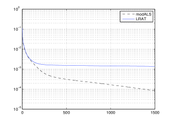
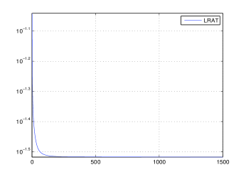
Figure 2 (a) demonstrates the residual function for the modALS and LRAT algorithms. Compared to the LRAT, the modALS executed by using five rank-one components decreases monotonically and has a low misfit on the residual function. Figure 2 (b) shows the objective function in (10) for the LRAT algorithm. It decreases monotonically and provides an estimate on the number of rank-one components as shown in Section 6.2, though the LRAT gave one less digit accuracy in the residual.
6.4 Application in surveillance video
Grayscale video data is a natural candidate for third-order tensors. Due to the correlation between subsequent frames of video, there exists some potential low-rank mechanism in the data. In this subsection, we apply the LRAT and the modALS to two surveillance videos111The original data is from http://perception.i2r.a-star.edu.sg/bk_model/bk_index.html on Fountain and Lobby. For each video of consecutive frames, we choose a region of interest with a resolution .
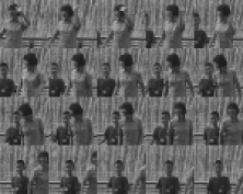
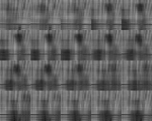

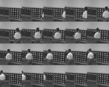


Figure 3 demonstrates simulation results on the LRAT and the modALS. Here the upper bound is fixed to . Figure 3 shows 20 frames in the original video data and those frames estimated by the LRAT and the modALS. The modALS provides an approximation with three factor matrices of elements. For the LRAT algorithm, the regularization parameter is set to , where and are computed as discussed in Section 5. The estimated number of rank-one components in is for the Fountain video. The representation of with three factor matrices only needs elements. The estimated number of rank-one components is for the Lobby video, and the representation with three factor matrices needs elements. Compared to the modALS algorithm, the LRAT has a smaller estimated rank but it sacrifices more cpu time, because the LRAT algorithm requires an instructive (a starter) choice on . For this case, we used the modALS algorithm to obtain a starter choice for LRAT.
7 Conclusion and future work
We propose an algorithm based on the proximal alternating minimization to detect the rank of tensors. This algorithm comes from the understanding of the low-rank approximation of tensors from sparse optimization. We also provide some theoretical guarantees on the convergence of this algorithm and a probabilistic consistency of the approximation result. Moreover, we suggest a way to choose a regularization parameter for practical computation. The simulation studies suggested that our algorithm can be used to detect the number of rank-one components in tensors.
The work presented in this paper have potential applications and extensions, especially in video processing and latent component number estimation. The ongoing work is to apply this low-rank approximation method to moving object detection and video data compression.
8 Acknowledgements
This work is in part supported by the National Natural Foundation of China 11401092.
References
- [1] E. Acar, D.M. Dunlavy, and T. Kolda, A scalable optimization approach for fitting canonical tensor decompositions, Journal of Chemometrics 25 (2):67-86, (2011).
- [2] C. Beckmann and S. Smith, Tensorial extensions of the independent component analysis for multisubject FMRI analysis, NeuroImage, 25 (2005), pp. 294-311.
- [3] D.P. Bertsekas, Nonlinear Programming, 2nd Edition, Athena Scientific, 1999
- [4] J. Bolte, S. Sabach and M. Teboulle, Proximal alternating linearized minimization nonconvex and nonsmooth problems, Mathematical Programming, 146 (2014), pp. 459-494.
- [5] J. Brachat, P. Comon, B. Mourrain and E. Tsigaridas Symmetric Tensor Decomposition, Linear Algebra and Applications 433, 11-12 (2010), pp. 1851-1872.
- [6] R. Bro, PARAFAC. Tuturial and applications, Chemometrics and Intelligent Laboratory Systems, 38 (1997), pp. 149-171.
- [7] E. J. Candès and Y. Plan, Near-ideal model selection by l1 minimization, Annals of Statistics, 37 (2007), pp. 2145-2177.
- [8] E. J. Candès J. Romberg and T. Tao, Robust uncertainty principles: exact signal reconstruction from highly incomplete frequency information, IEEE Trans. Inform. Theory, 52 (2004) 489-509.
- [9] E. J. Candès and T. Tao, Decoding by linear programming, IEEE Trans. Inform. Theory, 51 (2004) 4203-4215.
- [10] E. J. Candès, M. Wakin and S. Boyd, Enhancing sparsity by reweighted l1 minimization, J. Fourier Anal. Appl., 14 (2007), pp. 877-905.
- [11] P. Comon, Tensor decompositions, in Mathematics in Signal Processing V, J. G. McWhirter and I. K. Proudler, eds., Clarendon Press, Oxford, UK, 2002, pp. 1-24.
- [12] P. Comon, G. Golub, L.-H. Lim and B. Mourrain, Symmetric tensors and symmetric tensor rank, SIAM J. Matrix Anal. Appl., 30(3) (2008), 1254-1279.
- [13] L. De Lathauwer, B. De Moor and J. Vandevalle, A multilinear singular value decomposition, SIAM J. Matrix Anal. Appl., 21(4) (2000), pp. 1253-1278.
- [14] V. De Silva and L.-H. Lim, Tensor rank and the ill-posedness of the best low-rank approximation problem, SIAM J. Matrix Anal. Appl., 30 (2008), pp. 1084-1127.
- [15] I. Domanov and L.D. Lathauwer, Canonical polyadic decomposition of third-order tensors: reduction to generalized eigenvalue decomposition, SIAM J. Matrix Anal. Appl., 35 (2014), pp. 636-660.
- [16] D. Donoho, Compressed sensing, IEEE Trans. on Information Theory, 52(4) (2006), pp. 1289-1306.
- [17] C. Eckart and G. Young, The approximation of one matrix by another of lower rank, Psychometrika, 1 (1936), pp. 211-218.
- [18] S. Foucart and H. Rauhut, A Mathematical Introduction to Compressive Sensing, Birkhäuser, 2013.
- [19] G. Golub and C. F. Van Loan, Matrix Computations, Johns Hopkins University Press; 4th edition, 2013
- [20] N. Hao, M.E. Kilmer, K. Braman and R.C. Hoover, Facial recognition using tensor-tensor decompositions, SIAM J. Imaging Sciences, 6 (2013), pp. 437-463.
- [21] C.J. Hillar and L.-H. Lim, Most tensor problems are NP-hard, Journal of the ACM, 60 (2013), no. 6, Art. 45.
- [22] S. Karimi and S. Vavasis, IMRO: a proximal quasi-Newton method for solving -regularized least squares problem, manuscript, 2015.
- [23] M. Kilmer and D. O’Leary, Choosing regularization parameters in iterative methods for ill-Posed problems, SIAM J. Matrix Anal. Appl. 22 (4) pp. 1204-1221, 2001.
- [24] T.G. Kolda and B.W. Bader, Tensor decompositions and applications, SIAM Rev., 51 (2009), pp. 455-500.
- [25] T.G. Kolda, Orthogonal tensor decompositions, SIAM J. Matrix Anal. Appl., 23(1) (2001), pp. 243-255.
- [26] J.B. Kruskal, Three-way arrays: rank and uniqueness of trilinear decompositions, with applications to arithmetic complexity and statistics, Linear Algebra Appl., 18 (1977), pp. 95-138.
- [27] J. M. Landsberg, Tensors: Geometry and Applications, Graduate Studies in Mathematics, vol. 128, AMS, 2012.
- [28] N. Li, P. Hopke, P. Kumar, S. C. Cliff, Y. Zhao and C. Navasca, Source apportionment of time and size resolved ambient particulate matter, J. Chemometrics and Intelligent Laboratory Systems, 129, (2013), pp. 15-20, 2013.
- [29] L.-H. Lim and P. Comon, Nonnegative approximations of nonnegative tensors, Journal of Chemometrics, 23 (2009), pp. 432-441.
- [30] C.D. Martin, R. Shafer and B. Larue, An order-p tensor factorization with applications in imaging, SIAM J. Sci. Comput., 35 (2013), pp. A474-A490.
- [31] E. Martínez-Montes, P. Valdés-Sosa, F. Miwakeichi, R. Goldman, and M. Cohen, Concurrent EEG/fMRI analysis by multiway partial least squares, NeuroImage, 22 (2004), pp. 1023-1034.
- [32] V.A. Morozov, Regularization Methods for Ill-Posed Problems. CRC Press, Boca Raton, FL, 1993.
- [33] C. Navasca, L.D. Lathauwer and S. Kindermann Swamp reducing technique for tensor decomposition, in the 16th Proceedings of the European Signal Processing Conference, 2008.
- [34] P. Novati and M. R. Russo, A GCV based Arnoldi-Tikhonov regularization method, BIT Numerical Mathematics, 54 (2014), pp. 501-521.
- [35] B. Savas and L. Elden, Handwritten digit classification using higher order singular value decomposition, Pattern Recogn., 40 (2007), pp. 993-1003.
- [36] G. Schwarz, Estimating the dimension of a model, The annals of statistics, 6 (1978), pp. 461-464.
- [37] N. Sidiropoulos, R. Bro, and G. Giannakis, Parallel factor analysis in sensor array processing, IEEE Transactions on Signal Processing, 48 (2000), pp. 2377-2388.
- [38] M. Sorensen and L. De Lathauwer, Blind Signal Separation via Tensor Decomposition With Vandermonde Factor: Canonical Polyadic Decomposition, IEEE Transactions on Signal Processing, 61 (2013), pp. 5507-5519.
- [39] A. Uschmajew, Local convergence of the alternating least squares algorithm for canonical tensor approximation, SIAM J. Matrix Anal. Appl. 33(2):639-652, 2012.
- [40] E. van den Berg and M.P. Friedlander, Probing the Pareto frontier for basis pursuit solutions, SIAM J. Sci. Comput., 31 (2008), pp. 890-912.
- [41] M.J. Wainwright, Sharp thresholds for high-dimensional and noisy sparsity recovery using-constrained quadratic programming (Lasso), IEEE Transactions on Information Theory, 55 (2009), pp. 2183-2202.
- [42] Y. Xu and W. Yin, A block coordinate descent method for regularized multi-convex optimization with applications to nonnegative tensor factorization and completion, SIAM J. Imaging Sciences, 6 (2013), pp. 1758-1789.
- [43] P. Zhao and B. Yu, On model selection consistency of Lasso, Journal of Machine Learning Research, 7 (2006), pp. 2541-2567.