Smooth and sharp creation of a Dirichlet wall
in 1+1 quantum field theory: how singular
is the sharp creation limit?

Abstract

We present and utilize a simple formalism for the smooth creation of boundary conditions within relativistic quantum field theory. We consider a massless scalar field in $(1+1)$-dimensional flat spacetime and imagine smoothly transitioning from there being no boundary condition to there being a two-sided Dirichlet mirror. The act of doing this, expectantly, generates a flux of real quanta that emanates from the mirror as it is being created. We show that the local stress-energy tensor of the flux is finite only if an infrared cutoff is introduced, no matter how slowly the mirror is created, in agreement with the perturbative results of Obadia and Parentani. In the limit of instantaneous mirror creation the total energy injected into the field becomes ultraviolet divergent, but the response of an Unruh-DeWitt particle detector passing through the infinite burst of energy nevertheless remains finite. Implications for vacuum entanglement extraction and for black hole firewalls are discussed.

1 Introduction

Within the realm of relativistic quantum field theory, both in flat and curved spacetimes, the study of time-dependent boundary conditions has been a staple exercise in understanding particle-creation phenomena [1]. A non-inertially moving mirror, for example, induces the production of real particles out of the vacuum. Within a cavity setting this is commonly referred to as the dynamical Casimir effect [2], in which rapidly varying the length of an optical cavity can dynamically generate photons. This effect has been experimentally verified with a cQED analogue system [3]. Recently, there has been an increasing interest in utilizing the effect for quantum information processing and quantum metrology [4, 5, 6].

The majority of the existing literature is focused on the effects of moving boundaries. Here, we wish to properly examine a somewhat different case, and one that has been gaining interest in a number of areas. Rather than moving a boundary, we will instead create one. In particular, we take a $1+1$ dimensional massless scalar field and consider at the origin a self-adjointness boundary condition that transitions smoothly in time between there being no boundary to there being a two-sided Dirichlet wall. Physically, one can imagine such a procedure being implemented via a reflectivity-tunable barrier [7]. Unsurprisingly, such a procedure also generates quanta out of the vacuum that radiate away from the creation event. Our goal in this paper is to examine the stress-energy contribution to the field and the response of a particle detector. As part of this exposition we will take the limit of instantaneous wall creation.

There are several motivations behind studying such a scenario. For example, as has been pointed out by Unruh [8], the act of instantaneously creating a mirror produces regions of spacetime between which field correlations cannot propagate. On the horizon separating these regions (the future lightcone of the creation event) there is expected to be a flux of quanta of diverging energy density and diverging total energy (as we will confirm). Interestingly, this phenomenon is very analogous to the much-debated black hole firewall [9, 10, 11, 12, 13, 14, 15] and related constructs [16, 17, 18] in which lack of correlation between the inside and outside of a black hole is proposed to induce a violent horizon. Indeed, artificially constructing uncorrelated spatial regions has been used as a simplified firewall model [19, 20]. By considering the instantaneous limit of mirror creation within our formalism we are able to gain further insight into the nature of the divergence associated with firewalls.

The rapid creation of a mirror has recently gained further interest in studying the nature of vacuum entanglement [21, 22, 23]. It was shown in [21] that the two bursts of quanta produced by introducing a mirror are entangled with each other, and that this entanglement derives exactly from the previously present vacuum entanglement. The UV-divergent energy of these bursts is seen to be equivalent to the UV-divergence of the entanglement entropy between connected regions. This protocol has been proposed as a means of experimentally verifying vacuum entanglement. In any real experiment, however, the introduction of the mirror will take place over a finite time interval. In addition to theoretical insights into the sharp limit, considering a smooth transition (as we do here) may therefore prove vitally important for the development of such a program.

We have several goals in the current work, and give several different results of interest. First, we present a formalism for analysing a quantised massless scalar field in $(1+1)$-dimensional flat spacetime under time-dependent boundary conditions that are at each instant of time given by a specific self-adjoint extension of the spatial part of the wave equation [24, 25, 26], building on previous treatments in a variety of contexts [27, 28, 29, 30, 31, 32, 33, 34, 35, 36, 37, 38]. We use this formalism to analyse the smooth creation of a Dirichlet wall, both in full Minkowski space and at the centre of a Dirichlet cavity. We in particular compute the renormalized stress-energy expectation value in the quantum state in which no particles are present before the wall starts to form. In full Minkowski space, we find that the stress-energy is infrared divergent everywhere on the light cone of the evolving wall, no matter how slow the change in the boundary condition, as was previously observed within the perturbative analysis of [32] (for related observations in the back-reaction context see [29]): in full Minkowski space it is hence necessary to introduce an infrared cutoff by hand. For a wall that is forming within a cavity, by contrast, the stress-energy is finite without additional cut-offs since the cavity already provides an effective infrared cutoff.

Second, we consider the limit of instantaneous wall creation, by taking to zero the time interval over which the wall is created, while keeping fixed the dimensionless profile function by which the boundary condition evolves within this interval. We show that in this limit the stress-energy tensor vanishes everywhere except on the light cone of the wall creation event, but the limit is too singular for the stress-energy to be describable as a well-defined distribution with support on the light cone of the wall creation event, and in particular the total energy emitted into the field diverges. These outcomes are consistent with the instantaneous wall creation discussion in [8], with the instantaneous topology change discussion in [27, 28], with the perturbative discussion in [32] and with the conformal field theory discussion in [22].

Third, we compute the response of an Unruh-DeWitt particle detector [39, 40] that couples linearly to the proper time derivative of the field [19, 41, 42, 43, 44, 45, 46, 47], choosing the derivative coupling because it is less sensitive to the infrared ambiguity of the Wightman function of a $(1+1)$-dimensional massless field [46]. We take the detector to move inertially in full Minkowski spacetime. Working within first order perturbation theory, we find that in the instantaneous wall creation limit the detector’s response has two surprising properties. First, the response remains finite, despite the divergent total energy through which the detector passes. Second, the response depends on the infrared cutoff, even though the response in a number of other states, including the Minkowski vacuum, is independent of the infrared ambiguity [46]. These results are similar to what was found in [19, 20] for detectors coupled to a Minkowski spacetime model of a black hole firewall [9], and they add to the evidence that material systems modelled by the Unruh-DeWitt detector are significantly less sensitive to quantum field theoretic singularities than might be anticipated by considering just the local stress-energy of the field.

This paper is organized as follows. We begin in Section 2 with an introduction to the formalism and fully work out the evolution of the quantum field for wall creation that takes place smoothly over a finite interval of time in Minkowski space. We compute the stress-energy associated with this process, inserting by hand an infrared cutoff, and we show that the total energy diverges in the sharp creation limit. In Section 3 we perform the same analysis in the case of a Dirichlet cavity, demonstrating that the cavity acts as an infrared cutoff. In Section 4 we show that similar properties hold for creating a wall in Minkowski space over an infinite interval of time with a specific profile that allows computations to be done in terms of elementary functions. In Section 5 we go on to use this specific profile to analyse an inertial particle detector and to demonstrate, among other results, the response to remain finite even in the sharp-creation limit. Technical material is deferred to Appendices A–C. Appendix D presents a brief discussion of the wall creation in terms of Bogoliubov coefficients, both in Minkowski space and in the cavity.

We denote complex conjugation by an overline. $O(x)$ denotes a quantity such that $O(x)/x$ remains bounded as $x\to 0$, $O^{\infty}(x)$ denotes a quantity that goes to zero faster than any positive power of $x$ as $x\to 0$, and $O(1)$ denotes a quantity that remains bounded in the limit under consideration.

2 Wall creation in Minkowski spacetime

2.1 Classical field

We work in $(1+1)$-dimensional Minkowski spacetime, with standard global Minkowski coordinates $(t,x)$, in which the metric reads $ds^{2}=-dt^{2}+dx^{2}$. In the global null coordinates $u=t-x$ and $v=t+x$, the metric reads $ds^{2}=-du\,dv$.

We consider a real massless scalar field $\phi$. Without a wall, the field equation is the Klein-Gordon equation,

$$\partial_{t}^{2}\phi-\partial_{x}^{2}\phi=0\ ,$$ (2.1)

where $-\partial_{x}^{2}$ has its usual meaning as an essentially self-adjoint positive definite operator on $L_{2}(\mathbb{R})$.

To introduce a wall at $x=0$, we replace (2.1) with

$$\partial_{t}^{2}\phi-\Delta_{\theta(t)}\phi=0\ ,$$ (2.2)

where $\{-\Delta_{\theta}\mid\theta\in[0,\pi/2]\}$ is the one-parameter family of self-adjoint extensions of $-\partial_{x}^{2}$ on $L_{2}(\mathbb{R}\setminus\{0\})$ described in Appendix A. As indicated in (2.2), we allow $\theta$ to depend on $t$.

The special case $-\Delta_{\pi/2}$ is that of the unique self-adjoint extension of $-\partial_{x}^{2}$ on $L_{2}(\mathbb{R})$, corresponding to no wall at $x=0$. The special case $-\Delta_{0}$ is that of an impermeable wall at $x=0$ with the Dirichlet boundary condition on each side. For the intermediate values of $\theta$, $-\Delta_{\theta}$ interpolates between these two extremes, involving no boundary conditions for spatially odd wave functions but a two-sided Robin boundary condition [equation (A.3) in Appendix A] for spatially even wave functions.

The spectrum of each $-\Delta_{\theta}$ is the positive continuum. The wave equation (2.2) is hence free of tachyonic instabilities and provides a viable starting point for quantisation.

In physics terms, the wave equation (2.2) can be written for $0<\theta\leq\pi/2$ as

$$\left[\partial_{t}^{2}-\partial_{x}^{2}+\frac{2\cot\bigl{(}\theta(t)\bigr{)}}{L}\,\delta(x)\right]\phi=0\ ,$$ (2.3)

where $\delta(x)$ is Dirac’s delta-function and the positive constant $L$ of dimension length is as introduced in Appendix A. The wall at $x=0$ corresponds hence to a potential term proportional to $\delta(x)$ with a $\theta$-dependent coefficient. The coefficient is positive for $0<\theta<\pi/2$, and it tends to $0$ in the no-wall limit $\theta\to(\pi/2)_{-}$ and to $+\infty$ in the Dirichlet wall limit $\theta\to 0_{+}$.

In the rest of this section we assume that $\theta(t)$ interpolates between no wall and a fully-developed Dirichlet wall over a finite interval of time. We may assume without loss of generality that the wall creation begins at $t=0$, and we write the moment at which the Dirichlet wall is fully formed as $t=\lambda^{-1}$ where $\lambda>0$. We parametrise $\theta(t)$ as

$$\theta(t)=\begin{cases}\pi/2&\text{for $t\leq 0$}\ ,\\ \operatorname{arccot}\!\left[\lambda L\cot\bigl{(}h(\lambda t)\bigr{)}\right]&\text{for $0<t<\lambda^{-1}$}\ ,\\ 0&\text{for $t\geq\lambda^{-1}$}\ ,\end{cases}$$ (2.4)

where $h:\mathbb{R}\to\mathbb{R}$ is a smooth function such that

$$h(y)=\pi/2 \text{for $y\leq 0$}\ ,$$ (2.5a)

$$0<h(y)<\pi/2 \text{for $0<y<1$}\ ,$$ (2.5b)

$$h(y)=0 \text{for $y\geq 1$}\ .$$ (2.5c)

Over the interval $0<t<\lambda^{-1}$, the boundary condition (A.3) then reads

$$\lim_{x\to 0_{\pm}}\frac{\partial_{x}\phi(t,x)}{\phi(t,x)}=\pm\lambda\cot\bigl{(}h(\lambda t)\bigr{)}\ .$$ (2.6)

The parametrisation $\eqref{eq:theta-param}$ hence means that $\lambda^{-1}$ is the length of the time interval over which the boundary condition (2.6) evolves into Dirichlet, while the dimensionless function $h$ specifies the shape of the evolution in (2.6) over this time interval. The limit in which a wall is created rapidly but the shape of the evolution is held fixed is the limit of large $\lambda$ with fixed $h$.

We emphasise that the coefficient of $\delta(x)$ in (2.3) tends to $+\infty$ when the wall becomes a fully-developed Dirichlet wall, but the above description in terms of $\theta(t)$ nevertheless provides a control of the smoothness of this approach to the Dirichlet wall, and we shall verify in subsection 2.2 below that the mode functions indeed remain smooth even when the Dirichlet wall is reached. It would be possible to consider alternatives to (2.3), such as [32]

$$\left[\partial_{t}\bigl{(}1-\Lambda(t)\delta(x)\bigr{)}\partial_{t}-\partial_{x}^{2}\right]\phi=0\ ,$$ (2.7)

where $\Lambda(t)=0$ for $t\leq 0$ and $\Lambda(t)\to+\infty$ as $t\to\lambda^{-1}_{-}$; in particular, a potential advantage of (2.7) is that the wall is softer in the infrared, with implications for the stress-energy tensor [32]. For (2.7), one would however need to investigate anew the conditions on $\Lambda(t)$ as $t\to\lambda^{-1}_{-}$ to guarantee an appropriate sense of smoothness on reaching the Dirichlet wall.

2.2 Mode functions

As preparation for quantisation, we need to find the mode solutions that reduce to the usual Minkowski modes for $t\leq 0$, where the wall has not yet started to form.

Since the spatially odd solutions to the field equation (2.2) do not feel the wall, it suffices to consider the spatially even solutions. It further suffices to write down the expressions for these solutions in the half-space $x>0$; by spatial evenness, the expressions at $x<0$ follow by $(t,x)\mapsto(t,-x)$, or in terms of the null coordinates, by $(u,v)\mapsto(v,u)$.

We work in the null coordinates $(u,v)$ and look for the mode solutions with the ansatz

$$U_{k}(u,v)=\frac{1}{\sqrt{8\pi k}}\left[e^{-ikv}+E_{k}(u)\right]\ ,$$ (2.8)

where $k>0$ and $E_{k}$ is to be found. Each term in (2.8) satisfies the wave equation at $x>0$, and the left-moving part of $U_{k}$ has the standard form proportional to $e^{-ikv}$.

Requiring (2.8) to satisfy (A.3a) with $\theta=\theta(t)$ gives

$$L\sin\bigl{(}\theta(t)\bigr{)}\frac{d}{dt}\!\left[e^{-ikt}-E_{k}(t)\right] =\cos\bigl{(}\theta(t)\bigr{)}\!\left[e^{-ikt}+E_{k}(t)\right]\ .$$ (2.9)

With $\theta(t)$ parametrised by (2.4), the solution is

$$E_{k}(u)=R_{k/\lambda}(\lambda u)\ ,$$ (2.10)

with

$$R_{K}(y)=\begin{cases}{\displaystyle{e^{-iKy}}}&\text{for $y\leq 0$}\ ,\\ {\displaystyle{e^{-iKy}-\frac{2}{B(y)}\int_{0}^{y}{B^{\prime}}(y^{\prime})\,e^{-iKy^{\prime}}\,dy^{\prime}}}&\text{for $0<y<1$}\ ,\\[4.30554pt] {\displaystyle{-e^{-iKy}}}&\text{for $y\geq 1$}\ ,\end{cases}$$ (2.11)

where $B(y)$ is the solution to

$$\frac{B^{\prime}(y)}{B(y)}=\cot\bigl{(}h(y)\bigr{)}$$ (2.12)

for $0\leq y<1$ with the initial condition $B(0)=1$. An alternative expression for $R_{K}(y)$ for $0<y<1$ is

$$R_{K}(y)=-e^{-iKy}+\frac{2}{B(y)}-\frac{2iK}{B(y)}\int_{0}^{y}{B}(y^{\prime})\,e^{-iKy^{\prime}}\,dy^{\prime}\ .$$ (2.13)

Using (2.5) and the smoothness of $h$, it follows from (2.12) that $1/B(y)$ and all of its derivatives tend to zero as $y\to 1_{-}$, and this can be used to show from (2.13) that $R_{K}(y)$ is a smooth function of $y$ everywhere, including $y=1$. It follows that $E_{k}(u)$ is a smooth function of $u$.

At $u\leq 0$ and $u\geq\lambda^{-1}$, the mode functions $U_{k}$ reduce respectively to

$$U_{k}(u,v)=\begin{cases}{\displaystyle{\frac{1}{\sqrt{8\pi k}}\left[e^{-ikv}+e^{-iku}\right]}}&\text{for $u\leq 0$}\ ,\\[8.61108pt] {\displaystyle{\frac{1}{\sqrt{8\pi k}}\left[e^{-ikv}-e^{-iku}\right]}}&\text{for $u\geq\lambda^{-1}$}\ .\end{cases}$$ (2.14)

At $u\leq 0$, $U_{k}$ have not yet been affected by the wall, and they coincide with the usual spatially even mode functions in Minkowski, positive frequency with respect to $\partial_{t}$. At $u\geq\lambda^{-1}$, $U_{k}$ feel the fully-developed Dirichlet wall, and they coincide with the half-space mode functions with the Dirichlet boundary condition. In the interpolating region, $0<u<\lambda^{-1}$, $U_{k}$ are given by (2.8) with (2.10)–(2.12). The different regions are illustrated in Figure 1.

Recalling that the above formulas hold for $x>0$ and the corresponding formulas for $x<0$ are obtained by spatial evenness, it can be verified that $U_{k}$ satisfy the usual Klein-Gordon orthonormality relations

$$\bigl{(}U_{k},U_{k^{\prime}}\bigr{)} =\delta(k-k^{\prime})\ ,$$ (2.15a)

$$\bigl{(}\,\overline{U_{k}},\overline{U_{k^{\prime}}}\,\bigr{)} =-\delta(k-k^{\prime})\ ,$$ (2.15b)

$$\bigl{(}U_{k},\overline{U_{k^{\prime}}}\,\bigr{)} =0\ .$$ (2.15c)

where $(\,\cdot\,,\,\cdot\,)$ is the Klein-Gordon (indefinite) inner product [1].

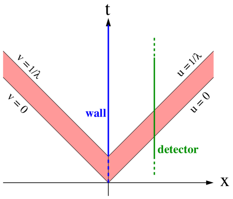
Figure 1: $(1+1)$-dimensional Minkowski spacetime with a wall evolving at $x=0$. The wall starts to evolve at $(t,x)=(0,0)$ and becomes a fully-developed two-sided Dirichlet wall at $(t,x)=(\lambda^{-1},0)$. The wall sends a pulse of energy that travels to the right in the null strip $0<u<\lambda^{-1}$ and to the left in the null strip $0<v<\lambda^{-1}$. The figure shows also the world line of an inertial detector at $x=d>0$.

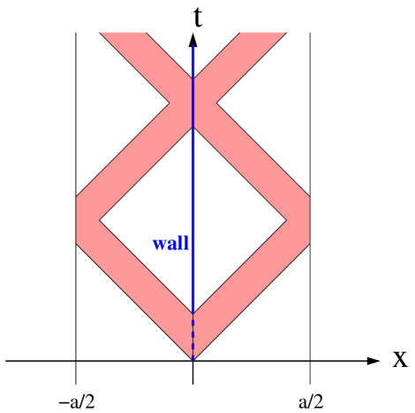
Figure 2: $(1+1)$-dimensional Dirichlet cavity of length $a$ with a wall evolving at the centre, $x=0$. The wall evolution is as in Figure 1, but the reflections from the boundaries at $x=\pm a/2$ affect the evolution of the mode functions for sufficiently late times. The figure shows the case $a>2/\lambda$, in which the Dirichlet wall at $x=0$ has fully formed before the changes in the field due to the wall evolution reach the boundaries at $(t,x)=(a/2,\pm a/2)$.

2.3 Quantisation and the rapid wall creation limit

We quantise the field in the usual fashion, adopting $U_{k}$ as the positive norm mode functions in the spatially even sector and the usual spatially odd Minkowski mode functions in the spatially odd sector. The spatially even part of $\phi$ is expanded as

$$\phi_{\text{even}}=\int_{0}^{\infty}\bigl{(}a_{k}U_{k}+a_{k}^{\dagger}\overline{U_{k}}\,\bigr{)}\,dk\ ,$$ (2.16)

where the nonvanishing commutators of the annihilation and creation operators are $\bigl{[}a_{k},a_{k^{\prime}}^{\dagger}\bigr{]}=\delta(k-k^{\prime})$. We denote by $|0_{M}\rangle$ the normalised state that is annihilated by all $a_{k}$ and by all the usual Minkowski annihilation operators of the spatially odd sector. $|0_{M}\rangle$ is indistinguishable from the usual Minkowski vacuum in the region $t<|x|$ which is outside the causal future of the wall.

We are interested in the energy that is transmitted into the quantum field by the evolving wall. Recall first that the classical stress-energy tensor of a massless minimally coupled scalar field is given by $T_{uu}=(\partial_{u}\phi)(\partial_{u}\phi)$, $T_{vv}=(\partial_{v}\phi)(\partial_{v}\phi)$ and $T_{uv}=0$ [1]. We point-split the quantised versions of these expressions and express their expectation values in $|0_{M}\rangle$ in terms of the Wightman function of the field, using (2.8) and (2.16). Subtracting the Minkowski contribution and taking the coincidence limit, we find that the renormalised stress-energy tensor $\langle T_{ab}\rangle$ is given by

$$\langle T_{vv}\rangle =\langle T_{uv}\rangle=0\ ,$$ (2.17a)

$$\langle T_{uu}\rangle =\int_{\mu}^{\infty}\frac{dk}{8\pi k}\left({\bigl{|}E^{\prime}_{k}(u)\bigr{|}}^{2}-k^{2}\right)\ ,$$ (2.17b)

where the constant $\mu$ is an infrared cutoff which we have inserted by hand.

When $\mu>0$, $\langle T_{uu}\rangle$ is well defined for all $u$, and vanishing for $u\leq 0$ and $u\geq\lambda^{-1}$, as is seen from (2.10) and (2.11). The convergence of the integral in (2.17b) at $k\to\infty$ for $0<u<\lambda^{-1}$ follows because ${\bigl{|}E^{\prime}_{k}(u)\bigr{|}}^{2}=k^{2}+O\bigl{(}k^{-2}\bigr{)}$ at large $k$, as can be verified by repeated integration by parts in (2.11), integrating the exponential factor [48]. When $\mu=0$, $\langle T_{uu}\rangle$ is still well defined and vanishing for $u\leq 0$ and $u\geq\lambda^{-1}$, but it is infrared divergent for $0<u<\lambda^{-1}$: this follows because for $0<u<\lambda^{-1}$ (2.10) and (2.13) give ${|E^{\prime}_{k}(u)|}^{2}=4\lambda^{2}{[{B^{\prime}}(\lambda u)]}^{2}{[B(\lambda u)]}^{-4}+O(k^{2})$ at small $k$, and (2.12) shows that ${B^{\prime}}(\lambda u){[B(\lambda u)]}^{-2}$ is nonvanishing. The infrared divergence was previously observed within a perturbative analysis in [32].

In words, this means that a positive infrared cutoff is required to make $\langle T_{ab}\rangle$ finite on the light cone of each wall point where the wall has started to form but has not yet reached the Dirichlet form. Where $\langle T_{ab}\rangle$ is nonzero, it corresponds to null radiation travelling away from the wall.

The total energy transmitted into the quantum field during the creation of the wall is

$$\langle E_{\text{tot}}\rangle =\int_{\Sigma}\langle T_{tt}\rangle\,dx$$

$$=2\int_{0}^{1/\lambda}\langle T_{uu}\rangle\,du\ ,$$ (2.18)

where for $\Sigma$ we may take any a constant $t$ hypersurface in the region $t>\lambda^{-1}$, and the last expression in (2.18) follows using (2.17) and by including the contribution from $x<0$. Inserting the solution (2.10)–(2.12) in (2.17), we find

$$\langle E_{\text{tot}}\rangle=\frac{\lambda}{4\pi}\int_{\mu/\lambda}^{\infty}\frac{dK}{K}\left(\int_{0}^{1}{\bigl{|}R^{\prime}_{K}(y)\bigr{|}}^{2}\,dy\ -K^{2}\right)\ .$$ (2.19)

For rapid wall creation, we consider the limit of large $\lambda$ with fixed $h$. Recall from (2.13) that for $0<y<1$ we have ${|R^{\prime}_{K}(y)|}^{2}=4{[{B^{\prime}}(y)]}^{2}{[B(y)]}^{-4}+O(K^{2})$, where the first term is bounded because $1/B(y)$ and its derivatives tend to zero as $y\to 1_{-}$. From (2.19) we hence obtain

$$\langle E_{\text{tot}}\rangle=\frac{\lambda}{\pi}\!\left(\ln(\lambda/\mu)\!\int_{0}^{1}\frac{{[{B^{\prime}}(y)]}^{2}}{{[B(y)]}^{4}}\,dy\ +O(1)\right)\ .$$ (2.20)

We conclude that in the rapid wall creation limit the energy transmitted into the quantum field diverges proportionally to $\lambda\ln(\lambda/\mu)$. The energy comes out as an increasingly narrow pulse near the light cone of the point $(t,x)=(0,0)$ but the magnitude of the pulse grows so rapidly that the stress-energy tensor does not have a distributional limit and the total energy diverges.

3 Wall creation within a Dirichlet cavity

In this section we adapt the analysis of Section 2 to a wall that is created at the centre of a static cavity whose left and right walls have time-independent Dirichlet boundary conditions. The main point of this adaptation is to verify that there is no need to introduce an infrared cutoff by hand since such a cutoff is already provided by the cavity.

3.1 Classical field and mode functions

Following the notation of Section 2, we confine the field $\phi$ to a static cavity whose walls are at $x=\pm a/2$, where the positive constant $a$ is the length of the cavity. We take $\phi$ to satisfy the Dirichlet boundary condition at $x=\pm a/2$.

At the centre of the cavity, $x=0$, we introduce the time-dependent boundary condition as in Section 2, with the same assumptions about $\theta(t)$. Again, the boundary condition does not affect the spatially odd part of the field, and it suffices to consider the spatially even part. We write down the formulas assuming $0<x<a/2$, with the spatial evenness providing the formulas for $-a/2<x<0$.

We look for the mode solutions with the ansatz

$$V_{n}(u,v)=\frac{1}{\sqrt{4\pi n}}\bigl{[}-F_{n}(v-a)+F_{n}(u)\bigr{]}\ ,$$ (3.1)

where the index $n$ is an odd positive integer and the function $F_{n}$ is to be found. This ansatz satisfies the wave equation at $0<x<a/2$, and it satisfies $V_{n}(u,a+u)=0$, which is the Dirichlet boundary condition at $x=a/2$.

Requiring (3.1) to satisfy (A.3a) with $\theta=\theta(t)$ gives

$$L\sin\bigl{(}\theta(t)\bigr{)}\frac{d}{dt}\left[F_{n}(t-a)+F_{n}(t)\right] =\cos\bigl{(}\theta(t)\bigr{)}\left[F_{n}(t-a)-F_{n}(t)\right]\ .$$ (3.2)

We again parametrise $\theta=\theta(t)$ by (2.4). We choose the solution that for $u<\min(a,\lambda^{-1})$ is given by

$$F_{n}(u)=R_{\pi n{(\lambda a)}^{-1}}(\lambda u)\ \ \text{for \ $u<\min(a,\lambda^{-1})$}\ ,$$ (3.3)

where $R_{K}$ is given by (2.11) and (2.12). For $u\leq 0$ this implies

$$V_{n}(u,v)=\frac{1}{\sqrt{4\pi n}}\bigl{[}e^{-i\pi nv/a}+e^{-i\pi nu/a}\bigr{]}\ \ \ \text{for $u\leq 0$}\ ,$$ (3.4)

so that at early times $V_{n}$ are the standard spatially even mode functions in the Dirichlet cavity. The domain $u<\min(a,\lambda^{-1})$, where the solution (3.3) holds, is where the time-dependence due to the evolving wall has not yet come back to $x=0$ after being reflected from $x=a/2$.

To evolve $F_{n}$ further to the future, one needs to account for the reflections of the time-dependence that start to arrive to $x=0$. The case of main interest for us is when $\lambda>a^{-1}$, which occurs when $a$ is considered fixed and we consider a rapid wall formation. In this case the Dirichlet wall at $x=0$ is fully formed when the first reflection due to the wall evolution arrives back to $x=0$. Equation (3.3) then holds for $u<\lambda^{-1}$, so that $F_{n}(u)=-e^{-i\pi nu/a}$ for $\lambda^{-1}\leq u\leq a$, and the evolution of $F_{n}(u)$ to $u>a$ is given just by successive Dirichlet reflections from $x=0$ and $x=a/2$. The case in which $\lambda>2/a$ is illustrated in Figure 2.

3.2 Quantisation and the rapid wall creation limit

We again quantise the field in the usual fashion and denote by $|0_{c}\rangle$ the vacuum with the above choice for the above positive norm mode functions. $|0_{c}\rangle$ is indistinguishable from the usual Dirichlet cavity vacuum in the region $t<|x|$, where its renormalised stress-energy tensor has the expectation value [1]

$$\langle T_{uu}\rangle_{\text{(early)}}=\langle T_{vv}\rangle_{\text{(early)}}=-\frac{\pi}{96\,a^{2}}\ ,$$ (3.5a)

$$\langle T_{uv}\rangle_{\text{(early)}}=0\ .$$ (3.5b)

To examine the stress-energy tensor due to the wall creation, we assume $\lambda>2/a$, and we consider the region $0<x<a/2$ and $t<a/2$, as illustrated in Figure 2. In this region the solution (3.3) holds, and the $v$-dependent part of $V_{n}$ has still the standard form proportional to $e^{-inv/a}$. Writing

$$\langle T_{ab}\rangle=\langle T_{ab}\rangle_{\text{(early)}}+\Delta\langle T_{ab}\rangle\ ,$$ (3.6)

we find

$$\Delta\langle T_{vv}\rangle =\Delta\langle T_{uv}\rangle=0\ ,$$ (3.7a)

$$\Delta\langle T_{uu}\rangle =\sum_{n>0\ \text{odd}}\frac{1}{4\pi n}\left[{\bigl{|}F^{\prime}_{n}(u)\bigr{|}}^{2}-{(\pi n/a)}^{2}\right]\ ,$$ (3.7b)

where the convergence of the sum in (3.7b) at large $n$ can be verified as in Section 2, and there is no infrared divergence because the sum starts at $n=1$. $\Delta\langle T_{uu}\rangle$ is vanishing for $u\leq 0$ and for $u\geq\lambda^{-1}$.

The total energy transmitted into the quantum field is given as in (2.18) but with $\langle T_{ab}\rangle$ replaced by $\Delta\langle T_{ab}\rangle$, and $\Sigma$ being now any constant $t$ hypersurface at $\lambda^{-1}<t<a/2$. Using (3.7b) with (3.3), we obtain

$$\langle E_{\text{tot}}\rangle=\frac{\lambda}{2\pi}\sum_{n>0\ \text{odd}}\frac{1}{n}\left[\int_{0}^{1}{\bigl{|}R^{\prime}_{\pi n{(\lambda a)}^{-1}}(y)\bigr{|}}^{2}\,dy\ -\left(\frac{\pi n}{\lambda a}\right)^{2}\right]\ .$$ (3.8)

In the limit of large $\lambda$, we may approximate the sum by an integral, and using the properties of $R_{K}$ as in Section 2 gives

$$\langle E_{\text{tot}}\rangle=\frac{\lambda}{\pi}\!\left[\ln\!\left(\frac{\lambda a}{\pi}\right)\int_{0}^{1}\frac{{[{B^{\prime}}(y)]}^{2}}{{[B(y)]}^{4}}\,dy\ +O(1)\right]\ .$$ (3.9)

The energy diverges proportionally to $\lambda\ln(\lambda a/\pi)$, and comparison with (2.20) shows that $\pi/a$ plays the role of an infrared cutoff. The divergence implies that the stress-energy tensor does not have a distributional limit at $\lambda\to\infty$.

4 Wall creation in Minkowski space over infinite time

In this section we adapt the Minkowski space analysis of Section 2 to a specific one-parameter family of wall evolution profiles for which the evolution is nontrivial at all finite times but reduces to no wall in the asymptotic past and to a wall with nonvanishing reflection and transmission coefficients in the asymptotic future. The main point is to verify that passing to an appropriate limit within this one-parameter family allows us again to model a rapid creation of a Dirichlet wall, and the results for the stress-energy tensor agree with those in Section 2. These properties will justify our use of this one-parameter family of evolution profiles with a particle detector in Section 5.

We take the boundary condition to be as in (2.6) with $\lambda$ a positive parameter and

$$h(y)=\arctan(1+e^{-y})\ ,$$ (4.1)

so that

$$\theta(t)=\arctan\!\left(\frac{1+e^{-\lambda t}}{\lambda L}\right)\ .$$ (4.2)

Since $0<\theta(t)<\pi/2$, the wall exists for all $t$, and it is never Dirichlet. Since $\theta(t)\to\pi/2$ as $t\to-\infty$, the wall disappears in the asymptotic past, and the wall formation starts exponentially slowly. Since $\theta(t)\to\operatorname{arccot}(\lambda L)$ as $t\to\infty$, the end state of the wall in the asymptotic future is not Dirichlet, but it can be made arbitrarily close to Dirichlet by taking $\lambda L$ large.

The parameter $\lambda$ has hence a dual role: it determines both how rapid the wall formation is and how close the wall is to Dirichlet in the asymptotic future. In the limit $\lambda\to\infty$, we approach the instantaneous creation of a Dirichlet wall at $t=0$.

We proceed as in Section 2. Equation (2.11) is now replaced by

$$R_{K}(y)=e^{-iKy}-\frac{2}{B(y)}\int_{-\infty}^{y}{B^{\prime}}(y^{\prime})\,e^{-iKy^{\prime}}\,dy^{\prime}\ ,$$ (4.3)

where (2.12) and the initial condition $B(y)\to 1$ as $y\to-\infty$ give

$$B(y)=1+e^{y}\ .$$ (4.4)

We find that $U_{k}$ is given by (2.8) with

$$E_{k}(u)=\frac{e^{-iku}}{1+e^{\lambda u}}\left[1-\left(\frac{\lambda+ik}{\lambda-ik}\right)e^{\lambda u}\right]\ .$$ (4.5)

For the stress-energy tensor, (2.17) gives

$$\langle T_{vv}\rangle =\langle T_{uv}\rangle=0\ ,$$ (4.6a)

$$\langle T_{uu}\rangle =\frac{\lambda^{2}}{32\pi\cosh^{4}(\lambda u/2)}\int_{\mu}^{\infty}\frac{dk}{k\left[1+{(k/\lambda)}^{2}\right]}$$

$$=\frac{\lambda^{2}\ln\!\left[1+{(\lambda/\mu)}^{2}\right]}{64\pi\cosh^{4}(\lambda u/2)}\ ,$$ (4.6b)

where the positive infrared cutoff $\mu$ is again needed to make $\langle T_{uu}\rangle$ finite.

When $\lambda\to\infty$, $\langle T_{uu}\rangle$ vanishes for $u\neq 0$ and diverges for $u=0$. To examine the strength of this divergence, we write

$$\langle T_{uu}\rangle =\frac{\lambda\ln\!\left[1+{(\lambda/\mu)}^{2}\right]}{24\pi}\,f_{\lambda}(u)\ ,$$ (4.7a)

$$f_{\lambda}(u) =\frac{3\lambda}{8\cosh^{4}(\lambda u/2)}\ ,$$ (4.7b)

and observe that $f_{\lambda}(u)\to\delta(u)$ as $\lambda\to\infty$. The divergence is hence too strong for $\langle T_{uu}\rangle$ to have a distributional limit. The total energy transmitted into the quantum field is

$$\langle E_{\text{tot}}\rangle =\lim_{t\to\infty}\int_{\Sigma_{t}}\langle T_{tt}\rangle\,dx$$

$$=\lim_{t\to\infty}2\int_{-\infty}^{t}\langle T_{uu}\rangle\,du$$

$$=\frac{\lambda\ln\!\left[1+{(\lambda/\mu)}^{2}\right]}{12\pi}\ ,$$ (4.8)

where $\Sigma_{t}$ is a hypersurface at constant $t$, and the final expression comes using (4.7) and observing that $\int_{-\infty}^{\infty}f_{\lambda}(u)\,du=1$. In the limit $\lambda\to\infty$, the energy diverges proportionally to ${(6\pi)}^{-1}\lambda\ln(\lambda/\mu)$ and comes out as a narrow burst near the light cone of $(t,x)=(0,0)$.

5 Response of an Unruh-DeWitt detector to rapid wall creation

In this section we consider the response of an inertial Unruh-DeWitt particle detector to the creation of a wall. We work in Minkowski spacetime with the wall creation profile (4.2). We are interested in the limit of large $\lambda$, in which the burst of energy from the wall diverges on the light cone of $(t,x)=(0,0)$. We ask what happens in the limit of large $\lambda$ to the response of a detector that crosses this light cone.

5.1 Detector and its trajectory

We consider a version of the Unruh-DeWitt detector [39, 40] that couples linearly to the proper time derivative of the field [19, 41, 42, 43, 44, 45, 46, 47]. Following the notation of [46], we denote by $\mathsf{x}(\tau)$ the detector’s worldline, parametrised by the proper time $\tau$. We assume that the coupling to the field is proportional to a real-valued function $\chi(\tau)$ that specifies how the interaction is turned on and off. We call $\chi$ the switching function and assume it to be smooth with compact support.

In first-order perturbation theory, the detector’s probability to make a transition from a state with energy $0$ to a state with energy $\omega$ is proportional to the response function, given by

$$\mathcal{F}^{(1)}(\omega) =\int^{\infty}_{-\infty}\,d\tau^{\prime}\,\int^{\infty}_{-\infty}\,d\tau^{\prime\prime}\,e^{-i\omega(\tau^{\prime}-\tau^{\prime\prime})}\,\chi(\tau^{\prime})\chi(\tau^{\prime\prime})\,\partial_{\tau^{\prime}}\partial_{\tau^{\prime\prime}}\mathcal{W}(\tau^{\prime},\tau^{\prime\prime})\ ,$$ (5.1)

where the correlation function $\mathcal{W}$ is the pull-back of the Wightman function to the detector’s worldline,

$$\mathcal{W}(\tau^{\prime},\tau^{\prime\prime}):=\langle\psi|\phi\bigl{(}\mathsf{x}(\tau^{\prime})\bigr{)}\phi\bigl{(}\mathsf{x}(\tau^{\prime\prime})\bigr{)}|\psi\rangle\ ,$$ (5.2)

and $|\psi\rangle$ is the state to which the field was initially prepared. The superscript ⁽¹⁾ in (5.1) is a reminder that the detector couples to the (first) derivative of the field. The derivatives in (5.1) are understood in the distributional sense, and integration by parts gives the alternative expression

$$\mathcal{F}^{(1)}(\omega) =\int_{-\infty}^{\infty}d\tau^{\prime}\int_{-\infty}^{\infty}d\tau^{\prime\prime}\,Q_{\omega}^{\prime}(\tau^{\prime})\overline{Q_{\omega}^{\prime}(\tau^{\prime\prime})}\,\mathcal{W}(\tau^{\prime},\tau^{\prime\prime})\ ,$$ (5.3)

where $Q_{\omega}(\tau):=e^{-i\omega\tau}\chi(\tau)$. $\mathcal{F}^{(1)}$ is hence well defined whenever $\mathcal{W}$ is a well-defined distribution.

We take the detector’s trajectory to be

$$(t,x)=(\tau+d,d)\ ,$$ (5.4)

where $d$ is a positive constant. The detector is inertial and it crosses the light cone of the origin at $(t,x)=(d,d)$. The zero of the proper time has been chosen to occur at this crossing. The geometry is shown in Figure 1.

5.2 Preliminaries: Minkowski vacuum and Dirichlet half-space

For comparisons to be made below, we record here the response in Minkowski vacuum and in Minkowski half-space with the Dirichlet boundary condition.

When there is no wall and the field is in the usual Minkowski vacuum, the response function is given by [19]

$$\mathcal{F}^{(1)}_{\text{Mink}}(\omega) =-\omega\Theta(-\omega)\int_{-\infty}^{\infty}du\,{[\chi(u)]}^{2}$$

$$\hskip 12.91663pt+\frac{1}{\pi}\int^{\infty}_{0}ds\,\frac{\cos(\omega s)}{s^{2}}\int_{-\infty}^{\infty}du\,\chi(u)[\chi(u)-\chi(u-s)]\ .$$ (5.5)

$\mathcal{F}^{(1)}_{\text{Mink}}$ is independent of the infrared cutoff, and its asymptotic form at large $|\omega|$ is [19]

$$\mathcal{F}^{(1)}_{\text{Mink}}(\omega) =-\omega\Theta(-\omega)\int_{-\infty}^{\infty}du\,{[\chi(u)]}^{2}\ +O^{\infty}\bigl{(}\omega^{-1}\bigr{)}\ .$$ (5.6)

When there is a static wall at $x=0$ and the field is in the usual vacuum state with Dirichlet conditions at this wall, we show in Appendix B that the response function is

$$\mathcal{F}^{(1)}_{\text{Dir}}=\mathcal{F}^{(1)}_{\text{Mink}}+\Delta_{\text{Dir}}\mathcal{F}^{(1)}\ ,$$ (5.7)

where

$$\Delta_{\text{Dir}}\mathcal{F}^{(1)}(\omega) =\frac{1}{2\pi}\operatorname{Re}\Biggl{\{}e^{-2i\omega d}\Biggl{[}i\pi G_{\omega}(2d)$$

$$\hskip 55.97205pt+\int_{0}^{\infty}ds\,\frac{e^{-i\omega s}G_{\omega}(2d+s)-e^{i\omega s}G_{\omega}(2d-s)}{s}\ \Biggr{]}\Biggr{\}}\ ,$$ (5.8a)

$$G_{\omega}(y) =\int_{-\infty}^{\infty}du\,\bigl{[}\chi^{\prime}(u)-i\omega\chi(u)\bigr{]}\chi(u-y)\ ,$$ (5.8b)

which is again independent of the infrared cutoff. We also show that the asymptotic large $|\omega|$ form of $\Delta_{\text{Dir}}\mathcal{F}^{(1)}$ is

$$\Delta_{\text{Dir}}\mathcal{F}^{(1)}(\omega) =\Theta(-\omega)\left[\omega\cos(2d\omega)\int_{-\infty}^{\infty}du\,\chi(u)\chi(u-2d)\right.$$

$$\hskip 51.6665pt\left.+\sin(2d\omega)\int_{-\infty}^{\infty}du\,\chi^{\prime}(u)\chi(u-2d)\right]\ +O^{\infty}\bigl{(}\omega^{-1}\bigr{)}\ .$$ (5.9)

5.3 Evolving wall

When the wall is present with the profile (4.2), we write the response function as

$$\mathcal{F}^{(1)}_{\lambda}=\mathcal{F}^{(1)}_{\text{Mink}}+\Delta\mathcal{F}^{(1)}_{\lambda}\ .$$ (5.10)

We show in Appendix C that $\Delta\mathcal{F}^{(1)}_{\lambda}$ has a finite limit as $\lambda\to\infty$, given by

$$\Delta\mathcal{F}^{(1)}(\omega) =\int^{\infty}_{-\infty}\,d\tau^{\prime}\,\int^{\infty}_{-\infty}\,d\tau^{\prime\prime}\,Q_{\omega}^{\prime}(\tau^{\prime})\overline{Q_{\omega}^{\prime}(\tau^{\prime\prime})}\,\Delta\mathcal{W}(\tau^{\prime},\tau^{\prime\prime})\ ,$$ (5.11)

where $\Delta\mathcal{W}(\tau^{\prime},\tau^{\prime\prime})$ is given by the following expressions:

$$\text{$\tau^{\prime}>0$, $\tau^{\prime\prime}>0$}: \ \ -\frac{1}{4\pi}\Bigl{[}E_{1}\bigl{(}\epsilon+i\mu(\tau^{\prime}-\tau^{\prime\prime}-2d)\bigr{)}+E_{1}\bigl{(}\epsilon+i\mu(\tau^{\prime}-\tau^{\prime\prime}+2d)\bigr{)}\Bigr{]}\ ,$$ (5.12a)

$$\text{$\tau^{\prime}>0$, $\tau^{\prime\prime}<0$}: \ \ -\frac{1}{4\pi}\Bigl{[}E_{1}\bigl{(}\epsilon+i\mu(\tau^{\prime}-\tau^{\prime\prime}-2d)\bigr{)}+E_{1}\bigl{(}\epsilon+i\mu(\tau^{\prime}-\tau^{\prime\prime})\bigr{)}\Bigr{]}\ ,$$ (5.12b)

$$\text{$\tau^{\prime}<0$, $\tau^{\prime\prime}>0$}: \ \ -\frac{1}{4\pi}\Bigl{[}E_{1}\bigl{(}\epsilon+i\mu(\tau^{\prime}-\tau^{\prime\prime})\bigr{)}+E_{1}\bigl{(}\epsilon+i\mu(\tau^{\prime}-\tau^{\prime\prime}+2d)\bigr{)}\Bigr{]}\ ,$$ (5.12c)

$$\text{otherwise}: \ \ \ 0\ .$$ (5.12d)

Here $\mu$ is the infrared cutoff and is assumed positive. $E_{1}$ is the exponential integral in the notation of [49], taking values on its principal branch in the sense of $\epsilon\to 0_{+}$. We further show in Appendix C that when $\omega+\mu\neq 0$, $\Delta\mathcal{F}^{(1)}$ can be put in the form

$$\Delta\mathcal{F}^{(1)}(\omega) =\frac{{[\chi(0)]}^{2}}{2\pi}\ln\bigl{|}1+(\omega/\mu)\bigr{|}$$

$$\hskip 12.91663pt-\frac{\omega}{2\pi}\int_{0}^{\infty}ds\,\frac{\sin\bigl{(}(\omega+\mu)s\bigr{)}}{s}\int_{0}^{s}du\,\chi(u)\chi(u-s)$$

$$\hskip 12.91663pt+\frac{1}{2\pi}\int_{0}^{\infty}ds\,\frac{\cos\bigl{(}(\omega+\mu)s\bigr{)}}{s}\left(\chi(0)\bigl{[}\chi(0)-\chi(-s)\bigr{]}-\int_{0}^{s}du\,\chi(u)\chi^{\prime}(u-s)\right)$$

$$\hskip 12.91663pt+\frac{1}{2\pi}\operatorname{Re}\Biggl{\{}e^{-2i\omega d}\Biggl{[}i\pi H_{\omega}(2d)$$

$$\hskip 64.58313pt+\int_{0}^{\infty}ds\,\frac{e^{-i(\mu+\omega)s}H_{\omega}(2d+s)-e^{i(\mu+\omega)s}H_{\omega}(2d-s)}{s}\ \Biggr{]}\Biggr{\}}\ ,$$ (5.13a)

$$H_{\omega}(y) =\int_{0}^{\infty}du\,\bigl{[}\chi^{\prime}(u)-i\omega\chi(u)\bigr{]}\chi(u-y)\ .$$ (5.13b)

Four observations are in order.

First, given that $\mu$ is assumed positive, equations (5.11) and (5.12) show that $\Delta\mathcal{F}^{(1)}$ is manifestly finite. The detector’s response remains finite when the wall creation becomes instantaneous, even though the detector passes through an infinite pulse of energy.

Second, $\Delta\mathcal{F}^{(1)}$ has a finite $\mu\to 0$ limit if and only if $\chi(0)=0$. This is seen from (5.13a) where the only potential divergence at $\mu\to 0$ comes from the first term. The infrared cutoff can hence be removed if and only if the detector does not operate at the moment of crossing the light cone of the wall creation event.

Third, as a consistency check, we note that if $\chi(\tau)$ vanishes for $\tau\leq 0$, the first three terms in (5.13a) vanish, and comparison of (5.13) and (5.8) shows that $\Delta\mathcal{F}^{(1)}$ reduces to $\Delta_{\text{Dir}}\mathcal{F}^{(1)}$ if $\mu$ is taken to zero. If the detector operates only after crossing the light cone of the wall creation event, the response is identical to that in a half-space with a static Dirichlet wall.

Fourth, we verify in Appendix C that the asymptotic form of $\Delta\mathcal{F}^{(1)}$ at large energy gap is

$$\Delta\mathcal{F}^{(1)}(\omega) =\frac{{[\chi(0)]}^{2}}{2\pi}\ln\bigl{(}e^{-1}\bigl{|}1+(\omega/\mu)\bigr{|}\bigr{)}$$

$$\hskip 12.91663pt+\Theta(-\omega-\mu)\left[\omega\cos(2d\omega)\int_{0}^{\infty}du\,\chi(u)\chi(u-2d)\right.$$

$$\hskip 81.8053pt\left.+\sin(2d\omega)\int_{0}^{\infty}du\,\chi^{\prime}(u)\chi(u-2d)\right]\ +O\bigl{(}\omega^{-1}\bigr{)}\ .$$ (5.14)

The terms proportional to $\omega\cos(2d\omega)$ and $\sin(2d\omega)$ are as expected from the corresponding terms in $\Delta_{\text{Dir}}\mathcal{F}^{(1)}$Z (5.9). The additional term, proportional to ${[\chi(0)]}^{2}$, comes strictly from the moment of crossing the light cone of the wall creation event. This term is dominant for $\omega\to\infty$ and subdominant for $\omega\to-\infty$.

6 Discussion

The purpose of this work has been to present a formalism for discussing the smooth creation of boundary conditions in quantum field theory, and to highlight some preliminary findings of interest. Specifically, we have examined several properties of the energy flux resulting from the smooth creation of a Dirichlet boundary condition for a massless scalar field in flat $(1+1)$-dimensional spacetime, and the resulting response of a particle detector. We have paid particular attention to the sharp creation limit of such a procedure. This type of scenario has gained interest recently from a number of different perspectives, and is markedly different from the more standard setting of a moving boundary condition. Our primary findings from this work are the following.

First, we have shown that the creation of a wall in Minkowski space induces an energy flux that is infrared divergent, regardless how slowly and smoothly the creation unfolds. This divergence was previously observed within a perturbative analysis in [32], and our results confirm that the divergence transcends the perturbative framework. While the Wightman function of the $(1+1)$-dimensional massless field is well known to be infrared divergent, it may be surprising that in our situation the infrared divergence shows up also in the stress-energy expectation value, which involves the Wightman function only through its derivatives. The upshot seems to be that in our time-dependent situation the infrared divergence of the Wightman function can no longer be thought of as an infinite additive constant but must be regarded as an infinite function, which does not drop out on taking a derivative. It should be interesting to give this phenomenon a more precise mathematical description, especially given its surprising and unintuitive nature.

Second, we have demonstrated that in the sharp creation limit (i.e. instantaneously producing a mirror) the resulting energy density flux is UV divergent, and diverges stronger than in any distributional sense. Thus, such a process would input an infinite amount of energy into the field. Indeed such a result is to be expected [8, 22, 27, 28, 32], and as demonstrated in [21] is related to the fact that the entanglement entropy between the two regions on either side of the created wall is UV divergent.

Third, we have considered the response of an inertial derivative-coupling Unruh-DeWitt detector that crosses the energy flux emitted from the wall creation. We showed that the detector’s response remains finite in the limit of instantaneous wall creation, despite the infinite amount of energy that the sharp creation injects into into the field. We also showed that in this sharp wall creation limit the detector’s response depends on the infrared cutoff, even though the derivative-coupling detector is known to be insensitive to the infrared ambiguity of the Wightman function in a number of other quantum states. Both of these properties are similar to the response of an inertial detector in a Minkowski spacetime model [19, 20] of a black hole firewall [9], and they add to the evidence that the prospective ability of a black hole firewall to resolve the black hole information paradox must hinge on the firewall’s detailed gravitational structure.

Our detector results were obtained in Section 5 under a specific one-parameter family of wall creation profiles. We conjecture that the same results for the sharp creation limit ensue within the full family of profiles introduced in Section 2. It is straightforward to verify that within this full family the pointwise sharp creation limit of the Wightman function is still given by (5.12); to justify the conjecture, it would remain to show that the sharp creation limit in the response function (5.3) can be taken pointwise under the integral. This question warrants further consideration.

An interesting next step would be to examine the entanglement structure between the bursts of particles generated by smooth wall creation, with the aim of showing how the formalism and results of [21] emerge in the sharp creation limit and comparing with the conformal field theory treatments of [22, 23]. As preparation for this analysis, we give in Appendix D the Bogoliubov coefficients between the field modes adapted to the boundary condition before and after the creation of the wall. Another next step would be to examine how this entanglement may be harvested by particle detectors. Conversely, it would be interesting to examine how pre-existing entanglement between particle detectors is affected by the wall creation, in the formalism that was applied to a Rindler firewall in [20].

Finally, we have throughout maintained that the quantum field lives on a nondynamical Minkowski metric even when the energy in the quantum field became infinite. Allowing the metric to become dynamical and to respond to the growing stress-energy could provide a model for a firewall in an evaporating black hole spacetime, in which the gravitational aspects near the horizon have had time to become significant.

Appendix A $-\partial_{x}^{2}$ on a line with a distinguished point

In this appendix we collect relevant properties about the self-adjoint extensions of the operator $-\partial_{x}^{2}$ on $L_{2}(\mathbb{R}\setminus\{0\})$. The general theory can be found for example in [24, 25] and a pedagogical summary in [26].

We take the coordinate $x$ to have the physical dimension of length. The self-adjoint extensions of $-\partial_{x}^{2}$ form a $U(2)$ family, specified by the boundary condition [26]

$$\begin{pmatrix}L\psi_{+}^{\prime}-i\psi_{+}\\ L\psi_{-}^{\prime}+i\psi_{-}\\ \end{pmatrix}=U\begin{pmatrix}L\psi_{+}^{\prime}+i\psi_{+}\\ L\psi_{-}^{\prime}-i\psi_{-}\\ \end{pmatrix}\ ,$$ (A.1)

where $\psi$ is the (generalised) eigenfunction, $\psi_{\pm}:=\lim_{x\to 0_{\pm}}\psi(x)$, $\psi^{\prime}_{\pm}:=\lim_{x\to 0_{\pm}}\psi^{\prime}(x)$, $L$ is a positive constant of dimension length and $U\in U(2)$. The constant $L$ has been introduced for dimensional convenience and its value is considered fixed. The extensions are then uniquely parametrised by the matrix $U\in U(2)$. Physically, $U$ encodes the reflection and transmission coefficients across $x=0$.

We specialise to the one-parameter subgroup of $U(2)$ given by

$$U(\theta)=e^{-i\theta}\begin{pmatrix}\cos\theta&i\sin\theta\\ i\sin\theta&\cos\theta\\ \end{pmatrix}\ ,\ \ \ \theta\in[0,\pi)\ ,$$ (A.2)

and we denote the corresponding self-adjoint extensions of $-\partial_{x}^{2}$ by $-\Delta_{\theta}$. If $\psi_{+}=\psi_{-}=0$ and $\psi^{\prime}_{+}=\psi^{\prime}_{-}$, (A.1) is satisfied as an identity. If $\psi_{+}=\psi_{-}$ and $\psi^{\prime}_{+}=-\psi^{\prime}_{-}$, (A.1) becomes

$$L\psi_{+}^{\prime}\sin\theta =\psi_{+}\cos\theta\ ,$$ (A.3a)

$$-L\psi_{-}^{\prime}\sin\theta =\psi_{-}\cos\theta\ .$$ (A.3b)

$-\Delta_{\theta}$ hence leaves the even and odd subspaces of $L_{2}(\mathbb{R}\setminus\{0\})$ invariant.

On the odd subspace of $L_{2}(\mathbb{R}\setminus\{0\})$, $-\Delta_{\theta}$ reduces to the unique self-adjoint extension of $-\partial_{x}^{2}$ on the odd subspace of $L_{2}(\mathbb{R})$. The generalised eigenfunctions are proportional to $\sin(kx)$ where $k>0$, and the spectrum is the positive continuum.

On the even subspace of $L_{2}(\mathbb{R}\setminus\{0\})$, $-\Delta_{\theta}$ is determined by the Robin boundary condition (A.3) on each side of $x=0$. When $0\leq\theta\leq\frac{1}{2}\pi$, the spectrum is the positive continuum, and the generalised eigenfunctions are proportional to $\sin(k|x|+\delta_{k})$ where $k>0$ and $\delta_{k}$ may be found in terms of $\theta$ from (A.3). When $\frac{1}{2}\pi<\theta<\pi$, the spectrum consists of the positive continuum, with the generalised eigenfunctions as above, together with the single negative proper eigenvalue $-\cot^{2}(\theta)/L^{2}$ [26].

We may summarise:

• On the odd subspace of $L_{2}(\mathbb{R}\setminus\{0\})$, $-\Delta_{\theta}$ involves no boundary condition and coincides with the unique self-adjoint extension of $-\partial_{x}^{2}$ on the odd subspace of $L_{2}(\mathbb{R})$.

• On the even subspace of $L_{2}(\mathbb{R}\setminus\{0\})$, $-\Delta_{\theta}$ is specified by the Robin boundary condition (A.3).

The following two cases have special interest.

When $\theta=\pi/2$, (A.3) reduces to Neumann on each side of $x=0$. $-\Delta_{\pi/2}$ hence coincides with the essentially self-adjoint operator $-\partial_{x}^{2}$ on $L_{2}(\mathbb{R})$. There is no boundary condition and the point $x=0$ has no special role.

When $\theta=0$, (A.3) reduces to Dirichlet on each side of $x=0$. Since the Dirichlet boundary condition is identically satisfied by odd wave functions, this means that $\mathbb{R}_{+}$ and $\mathbb{R}_{-}$ are completely decoupled by an impermeable two-sided Dirichlet wall at $x=0$.

Finally, we note that when $\theta\neq 0$, we may informally write

$$-\Delta_{\theta}=-\partial_{x}^{2}+{\frac{2\cot\theta}{L}}\,\delta(x)\ ,$$ (A.4)

where $\delta(x)$ is Dirac’s delta-function. In physics language, the boundary condition (A.1) with (A.2) can hence be described as a delta-function potential at $x=0$, with the $\theta$-dependent coefficient shown in (A.4). Our reason to describe $-\Delta_{\theta}$ in terms of $\theta$, rather than in terms of the coefficient of the Dirac delta in (A.4), is that this will allow us to control in the main text the regularity of the Dirichlet limit $\theta\to 0_{+}$, in which the coefficient of the Dirac delta in (A.4) tends to $+\infty$.

Appendix B Detector response in static half-space

In this appendix we verify the properties quoted in subsection 5.2 about the response of the inertial detector (5.4) in Minkowski half-space with Dirichlet boundary conditions.

In the Minkowski half-space $x>0$ with the Dirichlet boundary conditions at $x=0$, $\mathcal{W}(\tau^{\prime},\tau^{\prime\prime})$ consists of the Minkowski vacuum piece and the image contribution [46]

$$\Delta_{\text{Dir}}\mathcal{W}(\tau^{\prime},\tau^{\prime\prime})=\frac{1}{2\pi}\ln\Bigl{[}\mu\sqrt{(2d)^{2}-(\tau^{\prime}-\tau^{\prime\prime}-i\epsilon)^{2}}\,\Bigr{]}\ ,$$ (B.1)

where $\epsilon\to 0_{+}$. From (5.3) and (5.7) we then have

$$\Delta_{\text{Dir}}\mathcal{F}_{1}^{(1)}(\omega) =-\int_{-\infty}^{\infty}d\tau^{\prime\prime}\,\overline{Q_{\omega}^{\prime}(\tau^{\prime\prime})}\int_{-\infty}^{\infty}d\tau^{\prime}Q_{\omega}(\tau^{\prime})\,\partial_{\tau^{\prime}}\Delta_{\text{Dir}}\mathcal{W}(\tau^{\prime},\tau^{\prime\prime})\ .$$ (B.2)

After inserting (B.1) and writing out the $\tau^{\prime}$-derivative, the inner integral may be evaluated using the identity $\lim_{\epsilon\to 0_{+}}{(x-i\epsilon)}^{-1}=P(1/x)+i\pi\delta(x)$, where $P$ stands for the Cauchy principal value. Equations (5.8) in the main text then follow by writing out $\overline{Q_{\omega}^{\prime}(\tau^{\prime\prime})}=e^{i\omega\tau^{\prime\prime}}\bigl{[}\chi^{\prime}(\tau^{\prime\prime})+i\omega\chi(\tau^{\prime\prime})\bigr{]}$ and performing straightforward integration variable changes.

To obtain the large $|\omega|$ asymptotics, we assume $\omega\neq 0$ and rewrite (5.8a) as

$$\Delta_{\text{Dir}}\mathcal{F}_{1}^{(1)}(\omega) =\frac{1}{2\pi}\operatorname{Re}\Biggl{\{}e^{-2i\omega d}\Biggl{[}2i\pi G_{\omega}(2d)\Theta(-\omega)$$

$$\hskip 51.6665pt+\int_{0}^{\infty}ds\cos(\omega s)\,\frac{G_{\omega}(2d+s)-G_{\omega}(2d-s)}{s}$$

$$\hskip 51.6665pt-i\int_{0}^{\infty}ds\sin(\omega s)\,\frac{G_{\omega}(2d+s)+G_{\omega}(2d-s)-2G_{\omega}(2d)}{s}\ \Biggr{]}\Biggr{\}}\ ,$$ (B.3)

adding and subtracting a term proportional to $G_{\omega}(2d)$ and using the identity $\int_{0}^{\infty}ds\,s^{-1}\sin(\omega s)=\tfrac{1}{2}\pi\operatorname{sgn}\omega$ where $\operatorname{sgn}$ is the signum function. The method of repeated integration by parts, integrating the trigonometric factor [48], shows that the integral terms in (B.3) are $O^{\infty}\bigl{(}\omega^{-1}\bigr{)}$. Writing out $G_{\omega}(2d)$ gives formula (5.9) in the main text.

Appendix C Detector response for a rapidly created Dirichlet wall

In this appendix we verify the properties quoted in subsection 5.2 about the response of the inertial detector (5.4) for a wall created in Minkowski space with the profile (4.2).

C.1 Rapid wall creation limit

At $x>0$, the spatially even mode functions are given by (2.8) with (4.5), while without the wall the spatially even mode functions are given by (2.8) with $E_{k}(t)=e^{-ikt}$. From (5.10) we then have

$$\Delta\mathcal{F}_{\lambda}^{(1)}(\omega)=\int^{\infty}_{-\infty}\,d\tau^{\prime}\,\int^{\infty}_{-\infty}\,d\tau^{\prime\prime}\,Q_{\omega}^{\prime}(\tau^{\prime})\overline{Q_{\omega}^{\prime}(\tau^{\prime\prime})}\,\Delta\mathcal{W}_{\lambda}(\tau^{\prime},\tau^{\prime\prime})\ ,$$ (C.1)

where

$$\Delta\mathcal{W}_{\lambda}(\tau^{\prime},\tau^{\prime\prime}) =\frac{1}{4\pi\bigl{(}1+e^{-\lambda\tau^{\prime}}\bigr{)}\bigl{(}1+e^{-\lambda\tau^{\prime\prime}}\bigr{)}}\Bigl{[}2E_{1}\bigl{(}\mu(\epsilon+i\Delta\tau)\bigr{)}$$

$$\hskip 51.6665pt-e^{-\lambda\Delta\tau}E_{1}\bigl{(}(\mu+i\lambda)(\epsilon+i\Delta\tau)\bigr{)}-e^{\lambda\Delta\tau}E_{1}\bigl{(}(\mu-i\lambda)(\epsilon+i\Delta\tau)\bigr{)}\Bigr{]}$$

$$\hskip 8.61108pt-\frac{1}{4\pi\bigl{(}1+e^{-\lambda\tau^{\prime}}\bigr{)}}\Bigl{[}E_{1}\bigl{(}\mu(\epsilon+i\Delta\tau)\bigr{)}+E_{1}\bigl{(}\mu(\epsilon+i(\Delta\tau-2d))\bigr{)}$$

$$\hskip 86.11084pt-e^{-\lambda\Delta\tau}E_{1}\bigl{(}(\mu+i\lambda)(\epsilon+i\Delta\tau)\bigr{)}$$

$$\hskip 86.11084pt-e^{-\lambda(\Delta\tau-2d)}E_{1}\bigl{(}(\mu+i\lambda)(\epsilon+i(\Delta\tau-2d))\bigr{)}\Bigr{]}$$

$$\hskip 8.61108pt-\frac{1}{4\pi\bigl{(}1+e^{-\lambda\tau^{\prime\prime}}\bigr{)}}\Bigl{[}E_{1}\bigl{(}\mu(\epsilon+i\Delta\tau)\bigr{)}+E_{1}\bigl{(}\mu(\epsilon+i(\Delta\tau+2d))\bigr{)}$$

$$\hskip 86.11084pt-e^{\lambda\Delta\tau}E_{1}\bigl{(}(\mu-i\lambda)(\epsilon+i\Delta\tau)\bigr{)}$$

$$\hskip 86.11084pt-e^{\lambda(\Delta\tau+2d)}E_{1}\bigl{(}(\mu-i\lambda)(\epsilon+i(\Delta\tau+2d))\bigr{)}\Bigr{]}\ ,$$ (C.2)

$\Delta\tau:=\tau^{\prime}-\tau^{\prime\prime}$, the positive constant $\mu$ is an infrared cutoff, and $E_{1}$ is the exponential integral in the notation of [49], taking values on its principal branch in the sense of $\epsilon\to 0_{+}$.

We wish to take the limit $\lambda\to\infty$ in (C.1). For the terms in (C.2) that contain $\lambda$ in the argument of $E_{1}$, we may use properties of $E_{1}$ from [49] [the integral representation (6.2.1) and the asymptotic expansion (6.12.1)] to show that the contribution from these terms vanishes in the limit $\lambda\to\infty$. For the remaining terms in (C.2) the limit is elementary, leading to equations (5.11) and (5.12) in the main text.

C.2 Simplified expression (5.13) for the response function

We now express $\Delta\mathcal{F}^{(1)}$, given by (5.11) with (5.12), in terms of integrals that do not involve special functions.

Starting from (5.11) with (5.12) and breaking the integrations into subdomains gives

$$\Delta\mathcal{F}^{(1)}(\omega) =\Delta\mathcal{F}_{1}^{(1)}(\omega)+\Delta\mathcal{F}_{2}^{(1)}(\omega)\ ,$$ (C.3a)

$$\Delta\mathcal{F}_{1}^{(1)}(\omega) =-\frac{1}{2\pi}\operatorname{Re}\int_{0}^{\infty}d\tau^{\prime}\int_{-\infty}^{0}d\tau^{\prime\prime}\,Q_{\omega}^{\prime}(\tau^{\prime})\overline{Q_{\omega}^{\prime}(\tau^{\prime\prime})}\,E_{1}\bigl{(}i\mu(\tau^{\prime}-\tau^{\prime\prime})\bigr{)}\ ,$$ (C.3b)

$$\Delta\mathcal{F}_{2}^{(1)}(\omega) =-\frac{1}{2\pi}\operatorname{Re}\int_{0}^{\infty}d\tau^{\prime}\int_{-\infty}^{\infty}d\tau^{\prime\prime}\,Q_{\omega}^{\prime}(\tau^{\prime})\overline{Q_{\omega}^{\prime}(\tau^{\prime\prime})}\,E_{1}\bigl{(}i\mu(\tau^{\prime}-\tau^{\prime\prime}-2d)\bigr{)}\ ,$$ (C.3c)

where $E_{1}$ takes values on its principal branch.

Consider $\Delta\mathcal{F}_{1}^{(1)}$. In (C.3b), interchanging the integrals and integrating by parts in the inner integral gives

$$\Delta\mathcal{F}_{1}^{(1)}(\omega) =\Delta\mathcal{F}_{1,1}^{(1)}(\omega)+\Delta\mathcal{F}_{1,2}^{(1)}(\omega)\ ,$$ (C.4a)

$$\Delta\mathcal{F}_{1,1}^{(1)}(\omega) =\frac{\chi(0)}{2\pi}\operatorname{Re}\int_{-\infty}^{0}d\tau^{\prime\prime}\,\overline{Q_{\omega}^{\prime}(\tau^{\prime\prime})}\,E_{1}(-i\mu\tau^{\prime\prime})\ ,$$ (C.4b)

$$\Delta\mathcal{F}_{1,2}^{(1)}(\omega) =-\frac{1}{2\pi}\operatorname{Re}\int_{-\infty}^{0}d\tau^{\prime\prime}\,\overline{Q_{\omega}^{\prime}(\tau^{\prime\prime})}\int_{0}^{\infty}d\tau^{\prime}\,Q_{\omega}(\tau^{\prime})\,\frac{e^{-i\mu(\tau^{\prime}-\tau^{\prime\prime})}}{(\tau^{\prime}-\tau^{\prime\prime})}\ .$$ (C.4c)

From now on we assume $\omega+\mu\neq 0$.

To evaluate $\Delta\mathcal{F}_{1,1}^{(1)}$, we write $\Delta\mathcal{F}_{1,1}^{(1)}=\lim_{\epsilon\to 0_{+}}\Delta\mathcal{F}_{1,1,\epsilon}^{(1)}$, where $\Delta\mathcal{F}_{1,1,\epsilon}^{(1)}$ is as (C.4b) but with the upper limit of integration replaced by $-\epsilon$. Integrating by parts, renaming the integration variable by $\tau^{\prime\prime}=-s$, and adding and subtracting under the integral a term proportional to $e^{-i(\omega+\mu)s}/s$, we find

$$\Delta\mathcal{F}_{1,1,\epsilon}^{(1)}(\omega) =\frac{\chi(0)}{2\pi}\Biggl{\{}\int_{\epsilon}^{\infty}ds\,\frac{\chi(0)-\chi(-s)}{s}\cos\bigl{(}(\omega+\mu)s\bigr{)}$$

$$\hskip 12.91663pt+\operatorname{Re}\left[\chi(-\epsilon)e^{-i\omega\epsilon}E_{1}(i\mu\epsilon)\right]\ -\chi(0)\int_{\epsilon}^{\infty}\frac{ds}{s}\cos\bigl{(}(\omega+\mu)s\bigr{)}\Biggr{\}}\ .$$ (C.5)

The last term in (C.5) is proportional to the cosine integral $\operatorname{Ci}\bigl{(}|\omega+\mu|\epsilon\bigr{)}$ [49], and the limit $\epsilon\to 0_{+}$ can be taken using the small argument asymptotic forms of $\operatorname{Ci}$ and $E_{1}$ [49]. We find

$$\Delta\mathcal{F}^{(1)}_{1,1}(\omega) =\frac{{[\chi(0)]}^{2}}{2\pi}\ln\bigl{|}1+(\omega/\mu)\bigr{|}\ +\frac{\chi(0)}{2\pi}\int_{0}^{\infty}ds\,\frac{\chi(0)-\chi(-s)}{s}\cos\bigl{(}(\omega+\mu)s\bigr{)}\ .$$ (C.6)

To evaluate $\Delta\mathcal{F}_{1,2}^{(1)}$, we interchange the integrals in (C.4c), write $\overline{Q_{\omega}^{\prime}(\tau^{\prime\prime})}=e^{i\omega\tau^{\prime\prime}}\bigl{[}\chi^{\prime}(\tau^{\prime\prime})+i\omega\chi(\tau^{\prime\prime})\bigr{]}$, change the integration variable in the inner integral by $\tau^{\prime\prime}=\tau^{\prime}-s$ where $s\in(\tau^{\prime},\infty)$, and interchange the integrals again. Renaming $\tau^{\prime}$ as $u$, we find

$$\Delta\mathcal{F}^{(1)}_{1,2}(\omega) =-\frac{1}{2\pi}\int_{0}^{\infty}ds\cos\bigl{(}(\omega+\mu)s\bigr{)}\,s^{-1}\int_{0}^{s}du\,\chi(u)\chi^{\prime}(u-s)$$

$$\hskip 12.91663pt-\frac{\omega}{2\pi}\int_{0}^{\infty}ds\sin\bigl{(}(\omega+\mu)s\bigr{)}\,s^{-1}\int_{0}^{s}du\,\chi(u)\chi(u-s)\ .$$ (C.7)

Consider next $\Delta\mathcal{F}_{2}^{(1)}$. We change the integration variable in the inner integral in (C.3c) by $\tau^{\prime\prime}=\tau^{\prime}-2d-s$, interchange the integrals and rename $\tau^{\prime}$ as $u$, obtaining

$$\Delta\mathcal{F}_{2}^{(1)}(\omega) =-\frac{1}{2\pi}\operatorname{Re}\int_{-\infty}^{\infty}ds\,E_{1}(i\mu s)\int_{0}^{\infty}du\,Q_{\omega}^{\prime}(u)\overline{Q_{\omega}^{\prime}(u-2d-s)}$$

$$=\frac{1}{2\pi}\operatorname{Re}\left\{e^{-2i\omega d}\int_{-\infty}^{\infty}ds\,E_{1}(i\mu s)\,\frac{d}{ds}\bigl{[}e^{-i\omega s}H_{\omega}(2d+s)\bigr{]}\right\}\ ,$$ (C.8)

where $H_{\omega}$ is given by (5.13b). The last equality in (C.8) follows by observing that $\int_{0}^{\infty}du\,Q_{\omega}^{\prime}(u)\overline{Q_{\omega}^{\prime}(u-2d-s)}=-\frac{d}{ds}\int_{0}^{\infty}du\,Q_{\omega}^{\prime}(u)\overline{Q_{\omega}(u-2d-s)}$.

We may now write $\Delta\mathcal{F}_{2}^{(1)}=\lim_{\epsilon\to 0_{+}}\Delta\mathcal{F}_{2,\epsilon}^{(1)}$, where $\Delta\mathcal{F}_{2,\epsilon}^{(1)}$ is as in (C.8) except that the integration over $s$ omits the interval $(-\epsilon,\epsilon)$. Integration by parts gives

$$\Delta\mathcal{F}_{2,\epsilon}^{(1)}(\omega) =\frac{1}{2\pi}\operatorname{Re}\Biggl{\{}e^{-2i\omega d}\Biggl{[}E_{1}(-i\mu\epsilon)e^{i\omega\epsilon}H_{\omega}(2d-\epsilon)-E_{1}(i\mu\epsilon)e^{-i\omega\epsilon}H_{\omega}(2d+\epsilon)$$

$$\hskip 43.05542pt+\int_{-\infty}^{-\epsilon}ds\,\frac{e^{-i(\mu+\omega)s}}{s}H_{\omega}(2d+s)+\int_{\epsilon}^{\infty}ds\,\frac{e^{-i(\mu+\omega)s}}{s}H_{\omega}(2d+s)\ \Biggr{]}\Biggr{\}}\ .$$ (C.9)

The limit $\epsilon\to 0$ in (C.9) can be taken by using (6.2.4) of [49] in the first two terms and by the change of variables $s\to-s$ in the third term. We find

$$\Delta\mathcal{F}_{2}^{(1)}(\omega) =\frac{1}{2\pi}\operatorname{Re}\Biggl{\{}e^{-2i\omega d}\Biggl{[}i\pi H_{\omega}(2d)$$

$$\hskip 47.36096pt+\int_{0}^{\infty}ds\,\frac{e^{-i(\mu+\omega)s}H_{\omega}(2d+s)-e^{i(\mu+\omega)s}H_{\omega}(2d-s)}{s}\ \Biggr{]}\Biggr{\}}\ .$$ (C.10)

Combining (C.6), (C.7) and (C.10), we obtain formula (5.13) in the main text.

C.3 Limit of large energy gap

We now obtain the large $|\omega|$ form of $\Delta\mathcal{F}^{(1)}(\omega)$.

For $\Delta\mathcal{F}_{1}^{(1)}$, we apply to the integral terms in (C.6) and (C.7) the method of repeated integration by parts, integrating the trigonometric factor [48]. The second integral term in (C.7) is $-\frac{{[\chi(0)]}^{2}}{2\pi}+O\bigl{(}\omega^{-1}\bigr{)}$ and all the other integral terms are $O\bigl{(}\omega^{-1}\bigr{)}$. Combining, we have

$$\Delta\mathcal{F}_{1}^{(1)}(\omega) =\frac{{[\chi(0)]}^{2}}{2\pi}\ln\bigl{(}e^{-1}\bigl{|}1+(\omega/\mu)\bigr{|}\bigr{)}+O\bigl{(}\omega^{-1}\bigr{)}\ .$$ (C.11)

For $\Delta\mathcal{F}_{2}^{(1)}$, we apply to (C.10) the same method that was applied to (5.8a) in Appendix B. We obtain

$$\Delta\mathcal{F}_{2}^{(1)}(\omega) =\Theta(-\omega)\operatorname{Re}\bigl{[}ie^{-2i\omega d}H_{\omega}(2d)\bigr{]}\ +O^{\infty}\bigl{(}\omega^{-1}\bigr{)}\ .$$ (C.12)

Combining these observations and writing out $H_{\omega}(2d)$ gives formula (5.14) in the main text.

Appendix D Bogoliubov coefficients

In this appendix we examine briefly the wall creation in terms of Bogoliubov coefficients. We anticipate that this formalism will be useful for analysing the entanglement structure in the bursts of particles that the wall formation generates [21].

D.1 Wall in Minkowski space

Consider the wall creation in Minkowski spacetime, in the notation of Section 2. We recall that it suffices to consider the spatially even mode functions, and we write down the formulas for the mode functions only in the half-space $x>0$.

The mode functions that reduce to standard Minkowski mode functions before the wall starts to form are denoted by $U_{k}$ with $k>0$ and are given by (2.8) with (2.10)–(2.12). The mode functions that reduce to standard Minkowski mode functions with the Dirichlet boundary condition after the wall has fully formed are denoted by $W_{k}$ with $k>0$ and are given by

$$W_{k}(u,v)=\frac{1}{\sqrt{8\pi k}}\left[\tilde{E}_{k}(v)-e^{-iku}\right]\ ,$$ (D.1)

where

$$\tilde{E}_{k}(v)=e^{-ikv}\hskip 12.91663pt\text{for $v\geq\lambda^{-1}$}\ ,$$ (D.2)

and the expression for $\tilde{E}_{k}(v)$ for $v<\lambda^{-1}$ can be found by the methods of Section 2 but will not be needed here. $W_{k}$ satisfy the Klein-Gordon orthonormality relations similar to (2.15).

We write the Bogoliubov transformation between the two sets of modes in the notation of [1] as

$$W_{k}=\int_{0}^{\infty}\left(\alpha_{kl}U_{l}+\beta_{kl}\overline{U_{l}}\,\right)\,dl\ ,$$ (D.3)

so that

$$\alpha_{kl}=\bigl{(}W_{k},U_{l}\bigr{)}\ ,\ \ \ \ \beta_{kl}=-\bigl{(}W_{k},\overline{U_{l}}\,\bigr{)}\ .$$ (D.4)

The inner products in (D.4) may be evaluated by choosing a hypersurface of constant $t$ at $t\geq\lambda^{-1}$ and using (2.8) with (2.10)–(2.11) and (D.1) with (D.2). The result is

$$\alpha_{kl} =\frac{1}{2\pi}\sqrt{\frac{k}{l}}\left[i\,P\left(\frac{1+e^{i(l-k)/\lambda}}{l-k}\right)-\frac{1}{\lambda}\int_{0}^{1}e^{-i(k/\lambda)y}\,\overline{R_{l/\lambda}(y)}\,dy\right]\ ,$$ (D.5a)

$$\beta_{kl} =\frac{1}{2\pi}\sqrt{\frac{k}{l}}\left[i\,\frac{1+e^{-i(l+k)/\lambda}}{l+k}+\frac{1}{\lambda}\int_{0}^{1}e^{-i(k/\lambda)y}\,R_{l/\lambda}(y)\,dy\right]\ ,$$ (D.5b)

were $P$ denotes the Cauchy principal value. The presence of particle creation is manifest in the nonvanishing beta-coefficients (D.5b).

D.2 Wall in the Dirichlet cavity

For the wall creation in the Dirichlet cavity we may proceed similarly, in the notation of Section 3. We assume the cavity to be so large that $a>2/\lambda$.

For $\lambda^{-1}<t<a/2$, combining the results of Sections 2 and 3 shows that the $V$-modes (3.1) are obtained from the $U$-modes of (2.8) with (2.10)–(2.12) by including the overall multiplicative factor $\sqrt{2\pi/a}$ and restricting $ka/\pi$ to odd positive integers, while the $W$-modes are obtained from (D.1) with (D.2) by including the overall multiplicative factor $\sqrt{2\pi/a}$ and restricting $ka/\pi$ to even positive integers. The Bogoliubov transformation is written as in (D.4) but the integral replaced by a sum. It follows that the Bogoliubov coefficients are obtained from (D.5) by including the overall multiplicative factor $2\pi/a$, restricting $ka/\pi$ to even positive integers, restricting $la/\pi$ to odd positive integers, and dropping the symbol $P$. Again, the presence of particle creation is manifest in the nonvanishing beta-coefficients.

References

- [1] N. D. Birrell and P. C. W. Davies, Quantum Fields in Curved Space (Cambridge University Press, 1982).
- [2] G. Moore, “Quantum theory of electromagnetic field in a variable-length one-dimensional cavity,” J. Math. Phys. 11, 2679 (1970).
- [3] C. M. Wilson, G. Johansson, A. Pourkabirian, M. Simoen, J. R. Johansson, T. Duty, F. Nori and P. Delsing, “Observation of the dynamical Casimir effect in a superconducting circuit,” Nature 479, 376 (2011) [arXiv:1105.4714 [quant-ph]].
- [4] M. Ahmadi, D. E. Bruschi and I. Fuentes, “Quantum metrology for relativistic quantum fields” Phys. Rev. D 89, 065028 (2014) [arXiv:1312.5707 [quant-ph]].
- [5] G. Benenti, A. D’Arrigo, S. Siccardi and G. Strini, “Dynamical Casimir Effect in Quantum Information Processing”, Phys. Rev. D 90, 052313 (2014) [arXiv:1407.7567 [quant-ph]].
- [6] E. G. Brown, W. Donnelly, A. Kempf, R. B. Mann, E. Martín-Martínez and N. C. Menicucci, “Quantum seismology”, New J. Phys. 16, 105020 (2014) [arXiv:1407.0071 [quant-ph]].
- [7] S. R. Hastings, M. J. A. de Dood, H. Kim, W. Marshall, H. S. Eisenberg and D. Bouwmeester, “Ultrafast optical response of a high-reflectivity GaAs/AlAs Bragg mirror,” Appl. Phys. Lett. 86, 031109 (2005) [arXiv:cond-mat/0411312 [cond-mat.mtrl-sci]].
- [8] W. G. Unruh, “Firewalls — A gravitational perspective,” lecture at RQIN-2014 (Seoul, Korea, July 2014).
- [9] A. Almheiri, D. Marolf, J. Polchinski and J. Sully, “Black Holes: Complementarity or Firewalls?,” JHEP 1302, 062 (2013) [arXiv:1207.3123 [hep-th]].
- [10] L. Susskind, “Black Hole Complementarity and the Harlow-Hayden Conjecture,” arXiv:1301.4505 [hep-th].
- [11] A. Almheiri, D. Marolf, J. Polchinski, D. Stanford and J. Sully, “An Apologia for Firewalls,” JHEP 1309, 018 (2013) [arXiv:1304.6483 [hep-th]].
- [12] D. N. Page, “Excluding Black Hole Firewalls with Extreme Cosmic Censorship,” JCAP 1406, 051 (2014) [arXiv:1306.0562 [hep-th]].
- [13] A. Almheiri and J. Sully, “An uneventful horizon in two dimensions,” JHEP 1402, 108 (2014) [arXiv:1307.8149 [hep-th]].
- [14] M. Hotta, J. Matsumoto and K. Funo, “Black hole firewalls require huge energy of measurement,” Phys. Rev. D 89, 0124023 (2014) [arXiv:1306.5057 [quant-ph]].
- [15] D. Harlow, “Jerusalem Lectures on Black Holes and Quantum Information,” arXiv:1409.1231 [hep-th].
- [16] S. L. Braunstein, “Black hole entropy as entropy of entanglement, or it’s curtains for the equivalence principle,” arXiv:0907.1190v1 [quant-ph]; S. L. Braunstein, S. Pirandola and K. Zyczkowski, “Better Late than Never: Information Retrieval from Black Holes,” Phys. Rev. Lett. 110, 101301 (2013) [arXiv:0907.1190v3 [quant-ph]].
- [17] S. D. Mathur, “The information paradox: a pedagogical introduction,” Class. Quant. Grav. 26, 224001 (2009) [arXiv:0909.1038 [hep-th]].
- [18] J. Hutchinson and D. Stojkovic, “Icezones instead of firewalls: extended entanglement beyond the event horizon and unitary evaporation of a black hole,” arXiv:1307.5861 [hep-th].
- [19] J. Louko, “Unruh-DeWitt detector response across a Rindler firewall is finite,” JHEP 1409, 142 (2014) [arXiv:1407.6299 [hep-th]].
- [20] E. Martín-Martínez and J. Louko, “(1+1)D calculation provides evidence that quantum entanglement survives a firewall,” Phys. Rev. Lett. 115, 031301 (2015) [arXiv:1502.07749 [quant-ph]].
- [21] E. G. Brown, M. del Rey, H. Westman, J. León and A. Dragan, “What does it mean for half of an empty cavity to be full?,” Phys. Rev. D 91, 016005 (2015) [arXiv:1409.4203 [quant-ph]].
- [22] C. T. Asplund and A. Bernamonti, “Mutual information after a local quench in conformal field theory,” Phys. Rev. D 89, 066015 (2014) [arXiv:1311.4173 [hep-th]].
- [23] C. T. Asplund, A. Bernamonti, F. Galli and T. Hartman, “Holographic Entanglement Entropy from 2d CFT: Heavy States and Local Quenches,” JHEP 1502, 171 (2015) [arXiv:1410.1392 [hep-th]].
- [24] M. Reed and B. Simon, Methods of Modern Mathematical Physics II: Fourier Analysis, Self-adjointness (Academic, New York, 1975).
- [25] J. Blank, P. Exner and M. Havlíček, Hilbert Space Operators in Quantum Physics, 2nd edition (Springer, New York, 2008).
- [26] G. Bonneau, J. Faraut and G. Valent, “Selfadjoint extensions of operators and the teaching of quantum mechanics,” Am. J. Phys. 69, 322 (2001) [arXiv:quant-ph/0103153].
- [27] A. Anderson and B. S. DeWitt, “Does the topology of space fluctuate?,” Found. Phys. 16, 91 (1986).
- [28] C. A. Manogue, E. Copeland and T. Dray, “The trousers problem revisited,” Pramana 30, 279 (1988).
- [29] M. T. Jaekel and S. Reynaud, “Quantum fluctuations of mass for a mirror in vacuum,” Phys. Lett. A 180, 9 (1993) [arXiv:quant-ph/9801073].
- [30] A. P. Balachandran, G. Bimonte, G. Marmo and A. Simoni, “Topology change and quantum physics,” Nucl. Phys. B 446, 299 (1995) [arXiv:gr-qc/9503046].
- [31] D. Marolf, “Interpolating between topologies: Casimir energies,” Phys. Lett. B 392, 287 (1997) [arXiv:gr-qc/9602036].
- [32] N. Obadia and R. Parentani, “Notes on moving mirrors,” Phys. Rev. D 64, 044019 (2001) [arXiv:gr-qc/0103061].
- [33] J. R. Johansson, G. Johansson, C. M. Wilson and F. Nori, “Dynamical Casimir effect in superconducting microwave circuits,” Phys. Rev. A 82, 052509 (2010).
- [34] H. O. Silva and C. Farina, “A simple model for the dynamical Casimir effect for a static mirror with time-dependent properties,” Phys. Rev. D 84, 045003 (2011) [arXiv:1102.2238 [hep-th]].
- [35] C. Farina, H. O. Silva, A. L. C. Rego and D. T. Alves, “Time-dependent Robin boundary conditions in the dynamical Casimir effect,” Int. J. Mod. Phys. Conf. Ser. 14, 306 (2012) [arXiv:1201.3846 [quant-ph]].
- [36] A. L. C. Rego, J. P. d. S. Alves, D. T. Alves and C. Farina, “Relativistic bands in the spectrum of created particles via the dynamical Casimir effect,” Phys. Rev. A 88, 032515 (2013) [arXiv:1309.3159 [quant-ph]].
- [37] A. L. C. Rego, C. Farina, H. O. Silva and D. T. Alves, “New signatures of the dynamical Casimir effect in a superconducting circuit,” Phys. Rev. D 90, 025003 (2014) [arXiv:1405.3720 [quant-ph]].
- [38] J. Doukas and J. Louko, “Superconducting circuit boundary conditions beyond the dynamical Casimir effect,” Phys. Rev. D 91, 044010 (2015) [arXiv:1411.2948 [quant-ph]].
- [39] W. G. Unruh, “Notes on black hole evaporation,” Phys. Rev. D 14, 870 (1976).
- [40] B. S. DeWitt, “Quantum gravity: the new synthesis”, in General Relativity: an Einstein centenary survey, edited by S. W. Hawking and W. Israel (Cambridge University Press, Cambridge, 1979) 680.
- [41] D. J. Raine, D. W. Sciama and P. G. Grove, “Does an accelerated oscillator radiate?” Proc. Roy. Soc. A 435, 205 (1991).
- [42] A. Raval, B. L. Hu and J. Anglin, “Stochastic theory of accelerated detectors in a quantum field,” Phys. Rev. D 53, 7003 (1996) [arXiv:gr-qc/9510002].
- [43] P. C. W. Davies and A. C. Ottewill, “Detection of negative energy: 4-dimensional examples,” Phys. Rev. D 65, 104014 (2002) [arXiv:gr-qc/0203003].
- [44] Q. Wang and W. G. Unruh, “Motion of a mirror under infinitely fluctuating quantum vacuum stress,” Phys. Rev. D 89, 085009 (2014) [arXiv:1312.4591 [gr-qc]].
- [45] E. Martín-Martínez and J. Louko, “Particle detectors and the zero mode of a quantum field,” Phys. Rev. D 90, 024015 (2014) [arXiv:1404.5621 [quant-ph]].
- [46] B. A. Juárez-Aubry and J. Louko, “Onset and decay of the 1+1 Hawking-Unruh effect: what the derivative-coupling detector saw,” Class. Quant. Grav. 31, 245007 (2014) [arXiv:1406.2574 [gr-qc]].
- [47] M. Hotta, R. Schützhold and W. G. Unruh, “Partner particles for moving mirror radiation and black hole evaporation,” Phys. Rev. D 91, 124060 (2015) [arXiv:1503.06109 [gr-qc]].
- [48] R. Wong, Asymptotic Approximations of Integrals (Society for Industrial and Applied Mathematics, Philadelphia, 2001).
- [49] NIST Digital Library of Mathematical Functions. http://dlmf.nist.gov/, Release 1.0.9 of 2014-08-29.