HerMES: ALMA Imaging of Herschel^†-selected Dusty Star-forming Galaxies

Abstract

The Herschel Multi-tiered Extragalactic Survey (HerMES) has identified large numbers of dusty star-forming galaxies (DSFGs) over a wide range in redshift. A detailed understanding of these DSFGs is hampered by the limited spatial resolution of Herschel. We present 870$\,\mu$m 0$\farcs$45 resolution imaging from the Atacama Large Millimeter/submillimeter Array (ALMA) of 29 HerMES DSFGs with far-infrared (FIR) flux densities in between the brightest of sources found by Herschel and fainter DSFGs found in ground-based sub-millimeter (sub-mm) surveys. We identify 62 sources down to the $5\sigma$ point-source sensitivity limit in our ALMA sample ($\sigma\approx 0.2\,$mJy), of which 6 are strongly lensed (showing multiple images) and 36 experience significant amplification ($\mu>1.1$). To characterize the properties of the ALMA sources, we introduce and make use of uvmcmcfit, a publicly available Markov chain Monte Carlo analysis tool for interferometric observations of lensed galaxies. Our lens models tentatively favor intrinsic number counts for DSFGs with a steep fall off above 8 mJy at 880$\,\mu$m. Nearly 70% of the Herschel sources comprise multiple ALMA counterparts, consistent with previous research indicating that the multiplicity rate is high in bright sub-mm sources. Our ALMA sources are located significantly closer to each other than expected based on results from theoretical models as well as fainter DSFGs identified in the LABOCA ECDFS Submillimeter Survey. The high multiplicity rate and low projected separations argue in favor of interactions and mergers driving the prodigious emission from the brightest DSFGs as well as the sharp downturn above $S_{880}=8\,$mJy.

1. Introduction

Galaxies selected in blind surveys at far-infrared (FIR) or sub-millimeter (sub-mm) wavelengths are generally known as dusty star-forming galaxies (DSFGs; for a recent review, see Casey et al. 2014). They cover a wide range in redshift from $z\sim 0.5$ to $z>6$ (Chapman et al. 2005; Casey et al. 2012a; Messias et al. 2014; Riechers et al. 2013), with a significant component at $z\sim 2$ (Casey et al. 2012b; Bothwell et al. 2013), when they represent the most FIR-luminous objects in existence during this epoch. They are usually signposts of significant over-densities (Daddi et al. 2009; Capak et al. 2011) (c.f. Robson et al. 2014) and likely represent the formative stages of the most massive elliptical galaxies found in the local Universe (e.g., Ivison et al. 2013; Fu et al. 2013). Moreover, they constitute an important component of the overall galaxy population at $z\sim 2$ (e.g., Magnelli et al. 2011), when the star-formation rate density in the Universe peaked (e.g., Lilly et al. 1996; Madau et al. 1996).

Our collective understanding of DSFGs is currently taking a dramatic leap forward thanks in large part to the Herschel Space Observatory (Herschel; Pilbratt et al. 2010). Herschel has revolutized the size and depth of blind surveys at FIR wavelengths. In particular, the Herschel Multi-tiered Extragalactic Survey (HerMES; Oliver et al. 2012) and the Herschel Astrophysical Terahertz Large Area Survey (H-ATLAS; Eales et al. 2010) together have surveyed $\approx 650\,$deg² at 250$\,\mu$m, 350$\,\mu$m, and 500$\,\mu$m to the confusion limit of Herschel ($\sigma\approx 6-7\,$mJy in each band Nguyen et al. 2010), plus an additional $\approx 350\,$deg² to a shallower level (approximately double the confusion limit). A similar effort to survey large areas of the sky has been undertaken at longer wavelengths by the South Pole Telescope (SPT; Carlstrom et al. 2011) and the Atacama Cosmology Telescope (Swetz et al. 2011).

Theoretical expectations based on the redshift distribution and luminosity function of DSFGs suggested that HerMES and H-ATLAS would be efficient tools for discovering strongly lensed DSFGs (e.g., Blain 1996; Negrello et al. 2007). Submillimeter Array (SMA; Ho et al. 2004) imaging at 870$\,\mu$m with sub-arcsecond resolution has confirmed this, with $\geq 85\%$ of the brightest sources found by Herschel that satisfy $S_{500}>100\,$mJy being gravitationally lensed by an intervening galaxy or group of galaxies along the line of sight (Negrello et al. 2010; Conley et al. 2011; Riechers et al. 2011a; Bussmann et al. 2012; Wardlow et al. 2013; Bussmann et al. 2013). Sources discovered in SPT surveys have also been shown to have a high probability of being strongly lensed (Vieira et al. 2013; Hezaveh et al. 2013). However, statistical models significantly over-predict the median magnification factor experienced by a Herschel DSFG of a given $S_{500}$ (Bussmann et al. 2013). This could herald new insights in our understanding of the bright end of the intrinsic DSFG number counts or in the nature of the deflectors.

We here present Atacama Large Millimeter/submillimeter Array (ALMA) Cycle 0 imaging at 870$\,\mu$m of a sample of 29 HerMES DSFGs. Three aspects of our dataset make it uniquely suited to improving our understanding of the bright end of the intrinsic DSFG number counts. First, the sample occupies a distinct regime in flux density between the brightest Herschel DSFGs (almost all of which are lensed) and much fainter DSFGs found in ground-based surveys (most of which are expected to be unlensed; e.g., Hodge et al. 2013). Second, the ALMA images are extremely sensitive (rms point source sensitivity of $\sigma\approx 0.2\,$mJy) and all 29 HerMES DSFGs are detected (which was not the case in previous similar studies with shallower imaging; e.g., Smolčić et al. 2012; Barger et al. 2012; Hodge et al. 2013). Third, the typical angular resolution is $0\farcs 45$ and nearly all sources detected by ALMA are spatially resolved.

We also obtained Gemini-South optical imaging to complement our existing set of ancillary multi-wavelength imaging. We use those data in this paper to identify lensing galaxies, which are typically early-types with little on-going star-formation and therefore exhibit very weak sub-mm emission.

In Section 2, we characterize our sample and present our ALMA and Gemini-South imaging. Section 3 presents our model fitting methodology and model fits for all ALMA sources (lensed and unlensed) using uvmcmcfit, a publicly available modified version of the visibility plane lens modeling software used in Bussmann et al. (2012, 2013). Results on the effect of lensing for the observed properties of the Herschel DSFGs in our sample, as well as the multiplicity rate and typical angular separation between sources after delensing the ALMA sources, appear in Section 4. We scrutinize statistical predictions for the magnification factor at 870$\,\mu$m ($\mu_{870}$) as a function of the flux density at 870 $\,\mu$m ($S_{870}$) and discuss implications for the bright end of the DSFG number counts in Section 5. Finally, we present our conclusions in Section 6.

Throughout this paper, we assume a flat cosmology with $H_{0}=$69 km s^-1 Mpc^-1, $\Omega_{\rm m_{0}}=0.29$ (Hinshaw et al. 2013).

2. Data

In this section, we describe the selection of our Herschel DSFG sample, present our ALMA high-spatial resolution imaging of thermal dust emission, and present Gemini-S optical imaging that we use to identify intervening galaxies along the line of sight.

2.1. Selection of DSFG Sample

The starting point for the sample selection is source extraction and photometry. For the objects in this paper, individual catalogs were generated for each of the 250$\,\mu$m, 350$\,\mu$m, and 500$\,\mu$m Herschel Spectral and Photometric Imaging REceiver (SPIRE; Griffin et al. 2010) channels using the SUSSEXtractor peak finder algorithm (Savage & Oliver 2007). Our sample includes 29 DSFGs drawn from five independent, confusion-limited fields in HerMES with declinations below $+2^{\circ}$ and totaling $55\,$deg².

The sample was selected to be the 29 brightest DSFGs in the Southern sky that are not known radio AGN, nearby late-type galaxies, or Galactic emission. The selection was designed to assemble a large sample of lensed galaxies in the ALMA-accessible HerMES fields, and was constructed from the SUSSEXtractor catalogs (Smith et al. 2012), which were available prior to the ALMA Cycle 0 deadline. Subsequently, improved efforts to deblend SPIRE photometry at 500$\,\mu$m using StarFinder (Wang et al. 2014) were introduced that formed the basis of the lens selection criteria used in Wardlow et al. (2013). As a result of the improved deblending algorithms in the StarFinder catalogues and Wardlow et al. (2013) a number of objects in our sample have significantly lower $S_{500}$ values in the StarFinder catalog than in the original SUSSEXtractor catalogs. This and further investigation into the StarFinder catalogs shows that their original flux was boosted by blending with nearby sources rather than by gravitational lensing. For this reason, the objects in this sample comprise a combination of lenses and blends of multiple sources.

We used positional priors based on the ALMA data presented in this paper to obtain the best possible estimates of the total SPIRE flux densities for each Herschel source. We also used Spitzer/MIPS (Rieke et al. 2004) imaging to take into consideration the presence of nearby 24$\,\mu$m sources that are not detected by ALMA but may still contribute to the 250$\,\mu$m emission detected by Herschel. Additional details on our methodology are provided in Appendix A. The SPIRE flux densities measured in this way represent our “fiducial” flux densities and are presented in Table 1. Interested readers may refer to Table 5 for a comparison of the fiducial, StarFinder and SUSSEXtractor flux densities in tabular form.

Figure 1 shows that the Herschel-ALMA sample is set clearly apart from the very bright Herschel DSFGs that are selected to have $S_{500}>100\,$mJy and have been shown to be almost entirely lensed DSFGs (Negrello et al. 2010; Wardlow et al. 2013; Bussmann et al. 2013). In contrast, the sample in this paper is expected to include a mix of lensed and unlensed DSFGs. On the other hand, the HerMES survey area is 200 times larger than that of the Large Apex Bolometer Camera Extended Chandra Deep Field Survey (LESS Weiß et al. 2009). This explains why the median $S_{500}$ in our sample is $\sim 4$ times brighter than the median $S_{500}$ in the sample of ALMA-detected sources in LESS, known as ALESS (Swinbank et al. 2014). Our Herschel-ALMA sample opens a new window of discovery space on the bright end of the DSFG number counts.

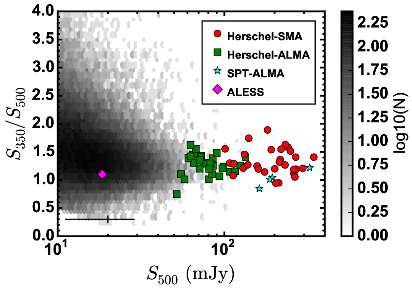
Figure 1.— Herschel/SPIRE photometry of all galaxies in the HerMES phase I catalog with declination $<+2\,^{\circ}$ and signal to noise ratio greater than 5 at 350$\,\mu$m and 500$\,\mu$m (log of number of galaxies shown in grayscale). The sample of HerMES sources in this paper are shown with green squares (“Herschel-ALMA”). The very bright Herschel DSFGs from Bussmann et al. (2013) (“Herschel-SMA”) are shown by red circles, and lensed SMGs discovered by the SPT that have published lens models (“SPT-ALMA”) are represented by cyan stars (Hezaveh et al. 2013). A magenta diamond shows the location in this diagram of the stacked signal from ALESS DSFGs. Representative error bars are shown in the lower left corner. The Herschel-ALMA sample fills the gap in 500$\,\mu$m flux density space between 50-100 mJy.

In detail, two of the sources in the Herschel-ALMA sample (HXMM01 and HXMM02) overlap with the “confirmed lensed” sample in Wardlow et al. (2013) as well as with the Herschel-SMA sample in Bussmann et al. (2013). A further eight appear in the “Supplementary sample” of Wardlow et al. (2013). The remainder have $S_{500}<80\,$mJy and thus do not appear in Wardlow et al. (2013).

Table 1 provides reference data for the Herschel-ALMA sample, including centroid positions measured from the ALMA 870$\,\mu$m imaging (see Section 2.2). The centroid positions serve as the reference point for subsequent offset positions of lenses and sources described in later tables. This is a useful choice (rather than the SPIRE centroid or ALMA phase center) because it minimizes the number of pixels needed to generate a simulated model of the source — and therefore minimized memory and cpu usage when lens modeling.

2.2. ALMA Observations

ALMA data were obtained during Cycle 0 over the from 2012 June to 2012 December (Program 2011.0.00539.S; PI: D. Riechers). The observations were carried out in good 870$\,\mu$m weather conditions, which resulted in typical system temperatures of $T_{\rm sys}\approx 130\,$K and phase fluctuations of $\sim 10\,^{\circ}$. Each target was observed until an rms point-source noise level near the phase center of $\sigma\approx 0.2\,$mJy per beam was achieved. This typically required 10 minutes of on-source integration time. For the observations targeting the CDFS, ELAISS, and COSMOS fields, the data reach $\sigma\approx 0.14\,$mJy per beam. The number of antennas used varied from 15 to 25. The antennas were configured with baseline lengths of 20 m to 400 m, providing a synthesized beamsize of $\approx 0\farcs 5\times 0\farcs 4$ FWHM while ensuring that no flux was resolved out by the interferometer (since our targets all have size scales smaller than $1\arcsec-2\arcsec$. When possible, track-sharing of multiple targets in a single track was used to optimize the uv coverage.

The quasars J0403$-$360, J2258$-$279, B0851$+$202, and J2258$-$279 were used for bandpass and pointing calibration. The quasars J0403$-$360, J0106$-$405, J0519$-$454, J1008$+$063, and J0217$+017$ were used for amplitude and phase gain calibration. The following solar system objects were used for absolute flux calibration: Callisto (CDFS targets); Neptune (XMM targets); Titan (COSMOS targets); and Uranus (ADFS and XMM targets). For HELAISS02, no solar system object was observed. Instead, J2258$-$279 was used for absolute flux calibration, with the flux fixed according to a measurement made two days prior to the observations of HELAISS02.

All observations were conducted with the correlator in “Frequency Domain Mode”, providing a total usable bandwidth of 7.5 GHz with spectral windows centered at 335.995 GHz, 337.995 GHz, 345.995 GHz, 347.996 GHz. We searched for evidence of serendipitous spectral lines but found none (typical sensitivity is $\sigma\approx 8\,$mJy beam^-1 in 15 km sec^-1 bins). Given that our observations cover a total of 217.5 GHz in bandwidth, the lack of lines seems more likely to be due to limited sensitivity than limited bandwidth.

We used the Common Astronomy Software Applications (CASA, version 4.2.1) package to re-reduce the data provided by the North American ALMA Science Center (NAASC). We found that the quality of the processed data from the NAASC was very high. However, we achieved a significant improvement in the case of the ADFS and XMM targets by excluding data sets with moderate $T_{\rm sys}$ and poor phase fluctuations. For a handful of targets with peak signal-to-noise ratio (S/N) greater than 20, we obtained a $\approx 10\%$ improvement in S/N by using the CASA selfcal task with the clean component model as input to improve the phase gain corrections. Finally, we updated the absolute flux calibration to use the Butler-JPL-Horizons 2012 solar system models .

For imaging, we used the CASA Clean task with Briggs weighting and “robust = $+$0.5” to achieve an optimal balance between sensitivity and spatial resolution. We selected the multi-frequency synthesis option to optimize uv coverage. We designed custom masks for each target in CASA to ensure that only regions with high S/N were considered during the cleaning process.

Figure 2 presents our ALMA images (color scale) in comparison to the Herschel SPIRE images (black-white contours) originally used to select the targets and noted in each panel as either 250$\,\mu$m, 350$\,\mu$m, or 500$\,\mu$m. Each panel is centered on the phase center of the ALMA observations of that target and a white circle traces the FWHM of the primary beam of an ALMA 12 m antenna at 870$\,\mu$m. All flux density measurements given in this paper have been corrected for the primary beam by dividing the total flux density by the primary beam correction factor at the center of the source. This is a valid approach because all sources have sizes $<1\arcsec$, such that the variation in the primary beam correction factor across the source is insignificant. A white dashed box represents the region of each image that is shown in greater detail in Figure 3.

In most targets, the peak of the SPIRE map is spatially coincident with the location of the ALMA sources. In one case where two ALMA sources are separated by $\approx 10\arcsec$ (HADFS08), the elongation in the SPIRE 250$\,\mu$m map is consistent with the angular separation of the two ALMA counterparts. Otherwise, the SPIRE imaging is consistent with a single component located at the centroid of the ALMA sources. This result is not a surprise, given the typical angular separation of the ALMA sources ($\lesssim 5\arcsec$) and the FWHM of the SPIRE beam at 250$\,\mu$m (18.1$\arcsec$). We identify and catalog by-eye all sources with peak flux density greater than 5$\sigma$.

2.3. Gemini-South Imaging

Optical imaging observations using the Gemini Multi-Object Spectrograph-South (GMOS-S; Hook et al. 2004) were conducted in queue mode during the 2013B semester as part of program GS-2013B-Q-77 (PI: R. S. Bussmann). The goal of the program is to use shallow $u$, $g$, $r$, $i$, and $z$ imaging to identify structure at redshifts below unity and determine which of the ALMA sources are affected by gravitational lensing. Nearly half of the ALMA sources lie in regions with existing deep optical imaging, thanks to the extensive multi-wavelength dataset available in the HerMES fields — these were excluded from our Gemini-S program. The remaining targets are: HADFS03, HADFS08, HADFS09, HADFS10, HADFS02, HADFS04, HADFS01, HADFS11, HELAISS02, HXMM11, HXMM12, HXMM22, HXMM07, HXMM30, and HXMM04. Each of these targets were observed for a total of 9 minutes of on-source integration time in each of $u$, $g$, $r$, $i$, and $z$. The observations were obtained during dark time in adequate seeing conditions (image quality in the 85th percentile, corresponding to $\approx 1.1\arcsec$).

The data were reduced using the standard IRAF Gemini GMOS reduction routines, following the standard GMOS-S reduction steps in the example taken from the Gemini observatory webpage .

We used the Sloan Digital Sky Survey (SDSS) or the 2 Micron All Sky Survey (2MASS) to align the Gemini-S images to a common astrometric frame of reference. This imposes an rms uncertainty in the absolute astrometry of $0\farcs 2$ and $0\farcs 4$ for SDSS and 2MASS, respectively. The astrometrically calibrated Gemini-S images served as the basis for aligning higher resolution, smaller field-of-view imaging from HST or Keck (when available), which were originally presented in Calanog et al. (2014).

Table 1Observed positions and flux densities of ALMA sources. For each Herschel source, we give the fiducial flux density in all SPIRE bands (see main text), as well as the observed positions and flux densities of all ALMA sources. The statistical rms and synthesized beam FWHM in each ALMA map ($\sigma_{\rm ALMA}$ and $\Omega_{\rm ALMA}$, respectively) are also given. Positional uncertainties (for unlensed sources) range from $\approx 0\farcs 005$ for well-detected sources to $\approx 0\farcs 15$ for the faintest soures in our sample. Uncertainties in flux density do not include the absolute calibration uncertainty of $\approx 10\%$. Quoted uncertainties in Herschel photometry are dominated by confusion noise (Nguyen et al. 2010).

		RA870	Dec870	$S_{250}$	$S_{350}$	$S_{500}$	$S_{870}$	$\sigma_{\rm ALMA}$	$\Omega_{\rm ALMA}$	Lens
IAU address	Short name	(J2000)	(J2000)	(mJy)	(mJy)	(mJy)	(mJy)	(mJy)	($\arcsec\times\arcsec$)	grade
J003823.6$-$433707	HELAISS02	00:38:23.587	$-$43:37:04.15	$115\pm 6$	$124\pm 6$	$108\pm 6$	$20.11\pm 0.45$	0.14	$0.54\times 0.44$	—
—	Source0	00:38:23.762	$-$43:37:06.10	—	—	—	$9.22\pm 0.17$	—	$---$	C
—	Source1	00:38:23.482	$-$43:37:05.56	—	—	—	$4.34\pm 0.16$	—	$---$	C
—	Source2	00:38:23.313	$-$43:36:58.97	—	—	—	$4.16\pm 0.32$	—	$---$	C
—	Source3	00:38:23.803	$-$43:37:10.46	—	—	—	$2.40\pm 0.19$	—	$---$	C
J021830.5$-$053124	HXMM02	02:18:30.673	$-$05:31:31.75	$78\pm 7$	$122\pm 8$	$99\pm 7$	$63.33\pm 0.58$	0.20	$0.49\times 0.37$	A
J021841.5$-$035002	HXMM31	02:18:41.613	$-$03:50:03.70	$102\pm 6$	$94\pm 6$	$65\pm 6$	$10.80\pm 0.46$	0.20	$0.49\times 0.37$	—
—	Source0	02:18:41.520	$-$03:50:04.72	—	—	—	$6.79\pm 0.37$	—	$---$	C
—	Source1	02:18:41.700	$-$03:50:02.57	—	—	—	$4.01\pm 0.26$	—	$---$	C
J021853.1$-$063325	HXMM29	02:18:53.111	$-$06:33:24.65	$97\pm 6$	$102\pm 6$	$78\pm 6$	$7.28\pm 0.45$	0.20	$0.49\times 0.37$	—
—	Source0	02:18:53.118	$-$06:33:24.19	—	—	—	$5.46\pm 0.30$	—	$---$	C
—	Source1	02:18:53.095	$-$06:33:25.21	—	—	—	$1.82\pm 0.38$	—	$---$	C
J021918.4$-$031051	HXMM07	02:19:18.417	$-$03:10:51.35	$89\pm 7$	$107\pm 8$	$85\pm 7$	$29.16\pm 0.58$	0.21	$0.49\times 0.38$	A
J021942.7$-$052436	HXMM20	02:19:42.783	$-$05:24:34.84	$72\pm 6$	$85\pm 6$	$66\pm 6$	$17.49\pm 0.74$	0.20	$0.49\times 0.37$	—
—	Source0	02:19:42.629	$-$05:24:37.11	—	—	—	$7.15\pm 0.44$	—	$---$	X
—	Source1	02:19:42.838	$-$05:24:35.11	—	—	—	$3.52\pm 0.41$	—	$---$	X
—	Source2	02:19:42.769	$-$05:24:36.48	—	—	—	$3.42\pm 0.26$	—	$---$	X
—	Source3	02:19:42.682	$-$05:24:36.82	—	—	—	$2.46\pm 0.47$	—	$---$	X
—	Source4	02:19:42.955	$-$05:24:32.22	—	—	—	$0.94\pm 0.18$	—	$---$	X
J022016.5$-$060143	HXMM01	02:20:16.609	$-$06:01:43.18	$179\pm 7$	$188\pm 8$	$134\pm 7$	$29.56\pm 0.46$	0.20	$0.48\times 0.37$	—
—	Source0	02:20:16.648	$-$06:01:41.93	—	—	—	$16.13\pm 0.31$	—	$---$	C
—	Source1	02:20:16.571	$-$06:01:44.56	—	—	—	$11.56\pm 0.32$	—	$---$	C
—	Source2	02:20:16.609	$-$06:01:40.72	—	—	—	$1.87\pm 0.26$	—	$---$	C
J022021.7$-$015328	HXMM04	02:20:21.756	$-$01:53:30.92	$162\pm 7$	$157\pm 8$	$125\pm 11$	$20.03\pm 0.47$	0.23	$0.53\times 0.38$	C
J022029.2$-$064845	HXMM09	02:20:29.140	$-$06:48:46.49	$129\pm 7$	$118\pm 8$	$85\pm 7$	$15.30\pm 0.36$	0.20	$0.49\times 0.37$	—
—	Source0	02:20:29.195	$-$06:48:48.02	—	—	—	$8.93\pm 0.30$	—	$---$	C
—	Source1	02:20:29.079	$-$06:48:44.86	—	—	—	$6.37\pm 0.19$	—	$---$	C
J022135.1$-$062617	HXMM03	02:21:34.891	$-$06:26:17.87	$114\pm 7$	$134\pm 8$	$116\pm 7$	$22.65\pm 0.36$	0.21	$0.48\times 0.38$	—
—	Source1	02:21:35.124	$-$06:26:16.62	—	—	—	$18.42\pm 0.36$	—	$---$	C
—	Source2	02:21:35.132	$-$06:26:18.02	—	—	—	$2.19\pm 0.20$	—	$---$	C
—	Source0	02:21:35.136	$-$06:26:17.28	—	—	—	$2.03\pm 0.18$	—	$---$	C
J022201.6$-$033340	HXMM11	02:22:01.616	$-$03:33:41.40	$101\pm 7$	$104\pm 8$	$73\pm 7$	$11.72\pm 0.49$	0.20	$0.52\times 0.38$	—
—	Source0	02:22:01.592	$-$03:33:39.42	—	—	—	$8.17\pm 0.32$	—	$---$	C
—	Source1	02:22:01.629	$-$03:33:43.58	—	—	—	$3.54\pm 0.36$	—	$---$	C
J022205.4$-$070728	HXMM23	02:22:05.362	$-$07:07:28.10	$128\pm 6$	$105\pm 6$	$68\pm 6$	$2.93\pm 0.15$	0.20	$0.48\times 0.37$	X
J022250.5$-$032410	HXMM22	02:22:50.573	$-$03:24:12.35	$101\pm 6$	$85\pm 6$	$61\pm 6$	$10.19\pm 0.28$	0.20	$0.49\times 0.38$	C
J022547.8$-$041750	HXMM05	02:25:47.942	$-$04:17:50.80	$103\pm 7$	$118\pm 8$	$97\pm 7$	$17.96\pm 0.43$	0.20	$0.50\times 0.37$	C
J022944.7$-$034110	HXMM30	02:29:44.740	$-$03:41:09.57	$86\pm 6$	$97\pm 6$	$75\pm 6$	$22.76\pm 0.28$	0.23	$0.50\times 0.38$	A
J023006.0$-$034152	HXMM12	02:30:05.950	$-$03:41:53.07	$98\pm 7$	$106\pm 8$	$82\pm 7$	$15.56\pm 0.37$	0.20	$0.50\times 0.38$	C
J032752.0$-$290908	HECDFS12	03:27:52.011	$-$29:09:10.40	$61\pm 7$	$82\pm 6$	$81\pm 6$	$38.78\pm 0.56$	0.15	$0.43\times 0.35$	—
—	Source0	03:27:52.002	$-$29:09:12.07	—	—	—	$16.76\pm 0.51$	—	$---$	A
—	Source1	03:27:52.002	$-$29:09:09.65	—	—	—	$14.55\pm 0.22$	—	$---$	C
—	Source2	03:27:52.025	$-$29:09:12.14	—	—	—	$7.47\pm 0.14$	—	$---$	X
J033210.8$-$270535	HECDFS04	03:32:10.840	$-$27:05:34.18	$56\pm 6$	$61\pm 6$	$55\pm 6$	$14.57\pm 0.26$	0.15	$0.44\times 0.35$	—
—	Source0	03:32:10.905	$-$27:05:32.87	—	—	—	$11.91\pm 0.24$	—	$---$	C
—	Source1	03:32:10.729	$-$27:05:36.22	—	—	—	$2.66\pm 0.11$	—	$---$	C
J033317.9$-$280907	HECDFS13	03:33:18.017	$-$28:09:07.52	$95\pm 6$	$89\pm 6$	$63\pm 6$	$15.36\pm 0.27$	0.14	$0.44\times 0.35$	—
—	Source0	03:33:18.006	$-$28:09:07.55	—	—	—	$10.11\pm 1.30$	—	$---$	X
—	Source1	03:33:18.032	$-$28:09:07.39	—	—	—	$5.25\pm 1.37$	—	$---$	X
J043340.5$-$540337	HADFS04	04:33:40.450	$-$54:03:39.51	$74\pm 6$	$93\pm 6$	$84\pm 6$	$18.12\pm 0.44$	0.19	$0.54\times 0.46$	—
—	Source0	04:33:40.455	$-$54:03:40.29	—	—	—	$9.25\pm 0.30$	—	$---$	C
—	Source1	04:33:40.501	$-$54:03:40.05	—	—	—	$6.09\pm 0.33$	—	$---$	C
—	Source2	04:33:40.472	$-$54:03:38.33	—	—	—	$2.78\pm 0.19$	—	$---$	C
J043619.3$-$552425	HADFS02	04:36:19.702	$-$55:24:25.01	$102\pm 6$	$97\pm 6$	$81\pm 5$	$16.79\pm 0.40$	0.19	$0.54\times 0.46$	—
—	Source0	04:36:19.706	$-$55:24:24.41	—	—	—	$7.81\pm 0.47$	—	$---$	X
—	Source1	04:36:19.698	$-$55:24:25.27	—	—	—	$8.99\pm 0.58$	—	$---$	X
J043829.7$-$541831	HADFS11	04:38:30.883	$-$54:18:29.38	$19\pm 6$	$39\pm 5$	$52\pm 6$	$28.47\pm 0.64$	0.19	$0.54\times 0.46$	—
—	Source0	04:38:30.780	$-$54:18:31.79	—	—	—	$21.19\pm 0.51$	—	$---$	C
—	Source1	04:38:30.970	$-$54:18:26.60	—	—	—	$7.28\pm 0.30$	—	$---$	C
J044103.8$-$531240	HADFS10	04:41:03.942	$-$53:12:41.01	$47\pm 6$	$58\pm 6$	$58\pm 6$	$17.44\pm 0.39$	0.20	$0.55\times 0.45$	—
—	Source0	04:41:03.866	$-$53:12:41.33	—	—	—	$9.61\pm 0.25$	—	$---$	X
—	Source1	04:41:04.000	$-$53:12:40.10	—	—	—	$4.59\pm 0.23$	—	$---$	X
—	Source2	04:41:03.912	$-$53:12:42.09	—	—	—	$3.24\pm 0.19$	—	$---$	X
J044153.9$-$540350	HADFS01	04:41:53.880	$-$54:03:53.48	$76\pm 6$	$100\pm 6$	$94\pm 6$	$32.79\pm 0.47$	0.19	$0.54\times 0.45$	A
J044946.9$-$525424	HADFS09	04:49:46.448	$-$52:54:26.95	$98\pm 6$	$102\pm 6$	$72\pm 6$	$15.52\pm 0.59$	0.19	$0.54\times 0.45$	—
—	Source0	04:49:46.603	$-$52:54:23.66	—	—	—	$8.24\pm 0.26$	—	$---$	X
—	Source1	04:49:46.301	$-$52:54:30.26	—	—	—	$4.86\pm 0.34$	—	$---$	X
—	Source2	04:49:46.280	$-$52:54:26.06	—	—	—	$2.42\pm 0.35$	—	$---$	X
J045026.5$-$524127	HADFS08	04:50:27.453	$-$52:41:25.41	$142\pm 6$	$133\pm 6$	$90\pm 6$	$14.18\pm 0.50$	0.19	$0.54\times 0.45$	—
—	Source0	04:50:27.092	$-$52:41:25.62	—	—	—	$6.17\pm 0.28$	—	$---$	C
—	Source1	04:50:27.806	$-$52:41:25.10	—	—	—	$8.01\pm 0.43$	—	$---$	C
J045057.5$-$531654	HADFS03	04:50:57.715	$-$53:16:54.42	$119\pm 6$	$102\pm 6$	$63\pm 6$	$11.50\pm 0.39$	0.19	$0.54\times 0.45$	—
—	Source0	04:50:57.610	$-$53:16:55.09	—	—	—	$7.12\pm 0.22$	—	$---$	C
—	Source1	04:50:57.805	$-$53:16:56.96	—	—	—	$2.12\pm 0.14$	—	$---$	C
—	Source2	04:50:57.741	$-$53:16:54.54	—	—	—	$2.27\pm 0.26$	—	$---$	C
J100056.6$+$022014	HCOSMOS02	10:00:57.180	$+$02:20:12.70	$70\pm 6$	$85\pm 6$	$71\pm 6$	$14.61\pm 0.66$	0.15	$0.63\times 0.50$	—
—	Source0	10:00:56.946	$+$02:20:17.35	—	—	—	$5.26\pm 0.26$	—	$---$	X
—	Source1	10:00:57.565	$+$02:20:11.26	—	—	—	$3.77\pm 0.32$	—	$---$	X
—	Source2	10:00:56.855	$+$02:20:08.93	—	—	—	$1.69\pm 0.25$	—	$---$	X
—	Source3	10:00:57.274	$+$02:20:12.66	—	—	—	$1.66\pm 0.21$	—	$---$	X
—	Source4	10:00:57.400	$+$02:20:10.83	—	—	—	$2.23\pm 0.41$	—	$---$	X
J100144.1$+$025712	HCOSMOS01	10:01:44.182	$+$02:57:12.47	$86\pm 6$	$96\pm 6$	$71\pm 6$	$15.35\pm 0.25$	0.14	$0.64\times 0.49$	A

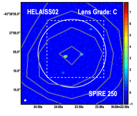
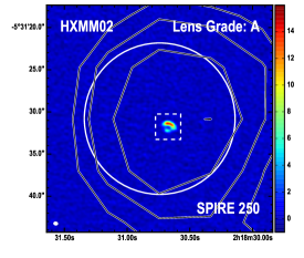
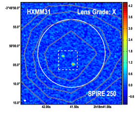
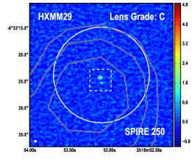
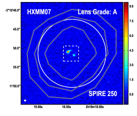
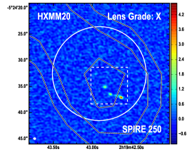
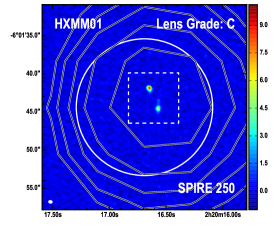
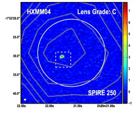
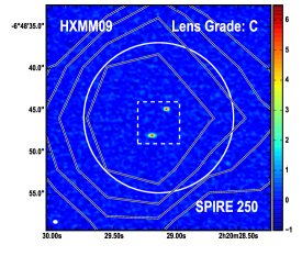
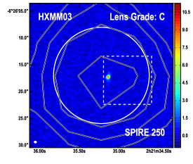
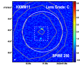
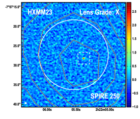
Figure 2.— ALMA 870$\,\mu$m images (color scale, units of mJy beam^-1) of HerMES DSFGs (images have not been corrected for primary beam attenuation). Contours (black and white) trace 250$\,\mu$m or 500$\,\mu$m emission from Herschel (starting at 4$\sigma$ and increasing by factors of 2, where $\sigma=7\,$mJy). North is up, east is left. The FWHM size of the ALMA synthesized beam is shown in the lower left corner of each panel. A solid white circle shows the FWHM size of the primary beam. Dashed squares identify the regions of each image that are shown in greater detail in Fig. 3.

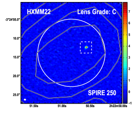
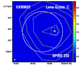
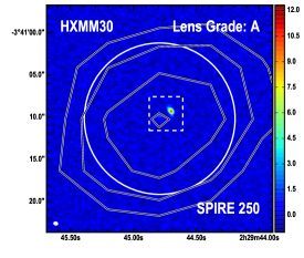
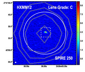
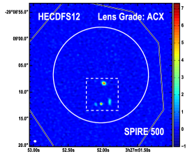
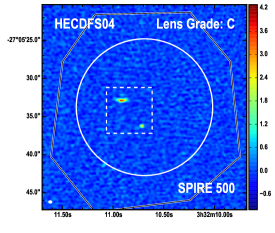
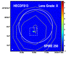
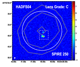
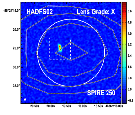
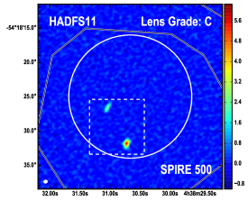
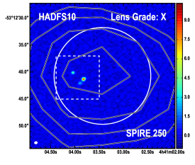
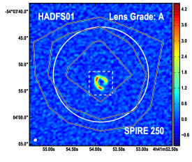
Figure 2.— Continued.

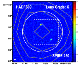
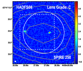
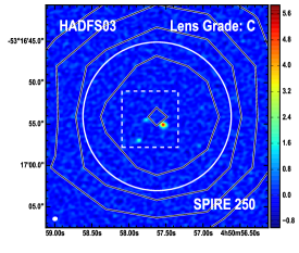
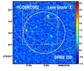
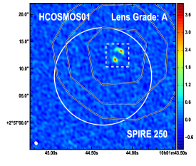
Figure 2.— Continued.

3. Model Fits

3.1. Model Fitting Methodology

An interferometer measures visibilities at discrete points in the uv plane. This is why pixel-to-pixel errors in the inverted and deconvolved surface brightness map of an astronomical source are correlated. The best way to deal with this situation is to compare model and data visibilities rather than surface brightness maps. The methodology used in this paper is similar in many aspects to that used in Bussmann et al. (2012), who presented the first lens model derived from a visibility-plane analysis of interferometric imaging of a strongly lensed DSFG discovered in wide-field submm surveys as well as in Bussmann et al. (2013), where this work was extended to a statistically significant sample of 30 objects. It also bears some resemblence to the method used in Hezaveh et al. (2013), who undertake lens modeling of interferometric data in the visibility plane. We summarize important information on the methodology here, taking care to highlight where any differences occur between this work and that of our previous efforts.

We created and made publicly available custom software, called uvmcmcfit, which is capable of modeling all of the ALMA sources in this paper efficiently.

Sources are assumed to be elliptical Gaussians that are parameterized by the following six free parameters: the position of the source (relative to the primary lens if a lens is present, $\Delta\alpha_{\rm s}$ and $\Delta\delta_{\rm s}$), the total intrinsic flux density ($S_{\rm in}$), the effective radius length ($r_{\rm s}=\sqrt{a_{\rm s}b_{\rm s}}$), the axial ratio ($q_{\rm s}$ = $b_{\rm s}/a_{\rm s}$), and the position angle ($\phi_{\rm s}$, degrees east of north). The use of an elliptical Gaussian represents a simplification from the Sérsic profile (Sersic 1968) that is permitted based on the relatively weak constraints on the Sérsic index found in our previous work (Bussmann et al. 2012, 2013).

When an intervening galaxy (or group of galaxies) is present along the line of sight, uvmcmcfit accounts for the deflection of light caused by this structure using a simple ray-tracing routine that is adopted from a Python routine written by A. Bolton . This represents a significant difference from Bussmann et al. (2012) and Bussmann et al. (2013), where we used the publicly available Gravlens software (Keeton 2001) to map emission from the source plane to the image plane for a given lensing mass distribution. Gravlens has a wide range of lens mass profiles as well as a sophisticated algorithm for mapping source plane emission to the image plane, but it also comes with a significant input/output penalty that makes parallel computing prohibitively expensive. For example, modeling a simple system comprising one lens and one source typically required 24-48 hours using the old software, whereas the same system can be modeled in less than one hour with the pure-Python code (tests of the Bolton ray-tracing routine indicate it produces results consistent with Gravlens). The use of pure-Python code for tracing the deflection of light rays is a critical component of making uvmcmcfit computationally feasible.

In uvmcmcfit, lens mass profiles are represented by $N_{\rm lens}$ singular isothermal ellipsoid (SIE) profiles, where $N_{\rm lens}$ is the number of lensing galaxies found from the best available optical or near-IR imaging (a multitude of evidence supports the SIE as a reasonable choice; for a review, see Treu 2010). Each SIE is fully described by the following five free parameters: the position of the lens on the sky relative to the arbitrarily chosen “image center” based on the ALMA 870$\,\mu$m emission and any lensing galaxies seen in the optical or near-IR ($\Delta\alpha_{\rm lens}$ and $\Delta\delta_{\rm lens}$; these can be compared with the position of the optical or near-IR counterpart relative to the “image center”: $\Delta\alpha_{\rm NIR}$ and $\Delta\delta_{\rm NIR}$), the mass of the lens (parameterized in terms of the angular Einstein radius, $\theta_{\rm E}$), the axial ratio of the lens ($q_{\rm lens}=b_{\rm lens}/a_{\rm lens}$), and the position angle of the lens ($\phi_{\rm lens}$; degrees east of north). Unless otherwise stated, when optical or near-IR imaging suggests the presence of additional lenses (see Figure 3), we estimate centroids for each lens by eye and fix the positions of the additional lenses with respect to the primary lens. Each additional lens thus has three parameters: $\theta_{\rm E}$, $q_{\rm lens}$, and $\phi_{\rm lens}$.

The total number of free parameters for any given system is $N_{\rm free}=5+3\times(N_{\rm lens}-1)+6*N_{\rm source}$, where $N_{\rm source}$ is the number of Gaussian profiles used.

We assume secondary, tertiary, etc., lenses are located at the same redshift as the primary lens. If this assumption were incorrect, to first order only the conversion from an angular Einstein radius to a physical mass of the lensing galaxy would be affected. As the physical masses of the lensing galaxies are not the focus of this work, this assumption is reasonable.

We use uniform priors for all model parameters. The prior on the position of the lenses covers $\pm 0\farcs 6$ ($1\farcs 0$) in both RA and Dec, a value that reflects the 1-$\sigma$ absolute astrometric solution between the ALMA and optical/near-IR images of $0\farcs 2$ ($0\farcs 4$) for SDSS-based (2MASS-based) astrometric calibration. In Section 3.2, we discuss the level of agreement between the astrometry from the images and the astrometry from the lens modeling on an object-by-object basis. For $\theta_{\rm E}$, the prior covers $0\farcs 1-6\arcsec$. The axial ratios of the lenses and sources are restricted to be $q_{\rm lens}>0.3$ and $q_{\rm s}>0.2$. This assumption is justified for the lenses because our optical observations reveal lenses that are not highly elliptical and because we expect dark matter to be more spherically distributed than the stars in lensing galaxies. For the sources, our ellipticity limit is primarily designed to aid numerical stability in the lens modeling. No prior is placed on the position angle of the lens or source. The intrinsic flux density for any source is allowed to vary from 0.1 mJy to the total flux density observed by ALMA (we ensure that the posterior PDF of the intrinsic flux density shows no signs of preferring a value lower than 0.1 mJy). The source position is allowed to vary over any reasonable range necessary to fit the data (typically, this is $\pm$1$\arcsec$-2$\arcsec$). The effective radius is allowed to vary from $0\farcs 01$-$1\farcs 5$.

The surface brightness map generated as part of uvmcmcfit is then converted to a “simulated visibility” dataset ($V_{\rm model}$) in much the same way as MIRIAD’s uvmodel routine. Indeed, the code used in uvmcmcfit is a direct Python port of uvmodel (the use of uvmodel itself is not possible for the same reason as Gravlens: constant input/output makes parallel computing prohibitively expensive). uvmcmcfit computes the Fourier transform of the surface brightness map and samples the resulting visibilities in a way that closely matches the sampling of the actual observed ALMA visibility dataset ($V_{\rm ALMA}$).

The goodness of fit for a given set of model parameters is determined from the maximum likelihood estimate $L$ according to:

$$L=\sum_{u,v}\left(\frac{|V_{\rm ALMA}-V_{\rm model}|^{2}}{\sigma^{2}}+{\rm log}(2\pi\sigma^{2})\right)$$ (1)

where $\sigma$ is the 1$\sigma$ uncertainty level for each visibility and is determined from the scatter in the visibilities within a single spectral window (this is a natural weighting scheme).

We use emcee (Foreman-Mackey et al. 2013) to sample the posterior probability density function (PDF) of our model parameters. emcee is a Markov chain Monte Carlo (MCMC) code that uses an affine-invariant ensemble sampler to obtain significant performance advantages over standard MCMC sampling methods (Goodman & Weare 2010).

We employ a “burn-in” phase with 512 walkers and 500-1000 iterations (i.e., $\approx 250,000-500,000$ samplings of the posterior PDF) to identify the best-fit model parameters. This position then serves as the basis to initialize the “final” phase with 512 walkers and 10 iterations (i.e., 5,120 samplings of the posterior PDF) to determine uncertainties on the best-fit model parameters.

During each MCMC iteration, we also measure the magnification factor at 870$\,\mu$m, $\mu_{870}$, for each source. This is done simply by taking the ratio of the total flux density in the lensed image of the model ($S_{\rm out}$) to the total flux density in the unlensed, intrinsic source model ($S_{\rm in}$). The use of an aperture when computing $\mu_{870}$ is important when source profiles are used with significant flux at large radii (e.g., some types of Sérsic profiles). For an elliptical Gaussian, such a step is unneccessary (note that we did test this and found only $\approx 10\%$ difference between $\mu_{870}$ computed with and without an aperture). The best-fit value and 1$\sigma$ uncertainty on $\mu_{870}$ are drawn from the posterior PDF, as with the other parameters of the model. Exceptions are made for cases of weakly lensed sources where we have only upper limits on the Einstein radius (and hence upper limits on $\mu_{870}$). In such instances, we re-compute $\mu_{870}$ as the arithmetic mean of the limiting $\mu_{870}$ and unity: $\mu_{870}=(\mu_{\rm 870-limit}+1)/2$. The uncertainty in $\mu_{870}$ is assumed to be equal to $\mu_{\rm 870-limit}-1)/2$.

Finally there are some important caveats to our approach. The spatial resolution of the ALMA observations is $\approx 0\farcs 45$, which is nearly always sufficient to resolve the images of the lensed galaxy, but not always sufficient to resolve the images themselves. For this reason, in some cases the lens models may moderately over-predict the intrinsic sizes of the lensed galaxies and hence under-predict the magnification factors. In addition, our Gemini-S optical imaging may have missed optically faint lenses due to being at high redshift or dust-obscured (but not sufficiently active to be detected by ALMA).

3.2. Individual Model Fits

In this section, we present our model fits (as shown in Figure 3) and describe each source in detail.

HELAISS02: Four sources are detected by ALMA, all of which are weakly lensed by a foreground galaxy seen in the HST image. To estimate the maximal magnification factors, we assume an Einstein radius of $1\farcs 5$ for the lens (larger values predict counter images that are not seen by ALMA). The ALMA sources are all detected by IRAC and their mid-IR colors are similar, suggesting that they lie at the same redshift (see Figure 4).

HXMM02: One source is detected by ALMA, and it is strongly lensed by one foreground galaxy seen in the HST image. The lensed source is not detected in the HST image. This object was first detected by Ikarashi et al. (2011) and also has high quality SMA imaging and an accompanying lens model that produces consistent results with those given here (Bussmann et al. 2013).

HXMM31: Two sources are detected by ALMA, neither of which are lensed. The faint, diffuse emission seen in the CFHT $i$-band image is atypical of lensing galaxies. The nearest bright galaxy seen at $i$-band is located $\approx 18\arcsec$ southeast of the ALMA sources.

HXMM29: Two sources are detected by ALMA, none of which appear to be lensed. The brighter ALMA source is weakly detected in the CFHT $i$-band image.

HXMM07: One source is detected by ALMA, and it is strongly lensed by one foreground galaxy detected in the Gemini-S image. There is a $\approx 0\farcs 5$ offset in the position of the foreground galaxy between the lens model and the Gemini-S image. Given the absolute astrometric rms uncertainty of $0\farcs 2$ (based on SDSS), we do not consider this offset to be significant. The presence of a handful of $\pm 3\sigma$ peaks in the residual map is likely an indication that our assumption of a single Gaussian to describe the source morphology is an oversimplification.

HXMM20: Five sources are detected by ALMA, none of which appear to be lensed. There are a few faint smudges seen in the HST image which are likely to be the rest-frame optical counterparts to the ALMA sources. The ALMA sources are all arranged in a chain like shape, possibly suggestive of a larger filamentary overdensity in which they might reside. IRAC imaging provides support for this hypothesis (see Figure 4), as all of the ALMA sources are detected and have similar mid-IR colors.

HXMM01: Three sources are detected by ALMA, all of which are weakly lensed by two foreground galaxies seen in the HST and Keck/NIRC2 imaging. The ALMA imaging is broadly consistent with SMA data originally presented in Fu et al. (2013), with two bright sources and a much fainter third source very close to the more southern bright source. We assume Einstein radii of $0\farcs 5$ for both lenses in order to reproduce the approach used in Fu et al. (2013). This results in magnification factors for the three sources of $\mu_{870}\approx 1.6-1.7$, consistent with Fu et al. (2013).

HXMM04: One source is detected by ALMA, and it is weakly lensed by a foreground galaxy seen in the HST image. We assume an Einstein radius of $0\farcs 5$ to represent the lensing scenario with maximum amplification. Due to the elliptical nature of the lens, this results in a maximum magnification factor of $\mu_{\rm 870-limit}=3.72\pm 0.42$. The HST morphology is complex: diffuse emission to the north of the lens could be a detection of the background source or could be a long spiral arm associated with the lensing galaxy.

HXMM09: Two sources are detected by ALMA, both of which are weakly lensed by a single foreground galaxy detected in the HST image. An Einstein radius of $1\farcs 5$ is used to represent the “maximal lensing” scenario and results in maximal magnification factors of $\mu_{\rm 870-limit}=2.25\pm 0.17$ and $\mu_{\rm 870-limit}=1.48\pm 0.09$.

HXMM03: Three sources are detected by ALMA, all of which are weakly lensed by a foreground galaxy detected in the HST image and located $\approx 6\arcsec$ from the ALMA sources. The central source is much brighter than the other two sources, which makes fitting a model challenging. We forced the positions of the second and third sources to be at least $0\farcs 5$ and $-0\farcs 5$ away from the first source in declination, respectively. Furthermore, we fixed the position of the lens to be located $2\farcs 5$ west and $0\farcs 5$ south of the image centroid given in Table 1. We also fixed the Einstein radius to be $1\farcs 0$, a typical value for isolated galaxies in this sample and in Bussmann et al. (2013). Because the source is so far from the lens, the maximal magnification factor is only $\mu_{\rm 870-limit}=2.0\pm 0.1$.

HXMM11: Two sources are detected by ALMA, both of which are weakly lensed. This system is similar to HADFS08, although the two ALMA sources are much closer and the lens must be less massive in order to avoid producing multiple images of the closest ALMA source. The fainter ALMA source has a much lower maximal magnification factor than the brighter source ($\mu_{\rm 870-limit}=1.10\pm 0.01$ vs. $\mu_{\rm 870-limit}=1.63\pm 0.11$). Both ALMA sources are detected by IRAC and have similar mid-IR colors, suggesting they lie at similar redshifts (see Figure 4).

HXMM23: One source is detected by ALMA, and it is coincident (within the astrometric uncertainty) with a late-type galaxy seen in the HST image. Here, we assume that the HST source is the true counterpart to the ALMA source, implying that no lensing is occuring. Consistent with this hypothesis is that the SPIRE photometry show blue colors that suggest this object is at low redshift. Note that models in which the late-type galaxy is lensing the ALMA source by a modest amount ($\mu_{870}<1.2$) cannot be ruled out with the present data.

HXMM22: One source is detected by ALMA, and it appears to be unlensed. A faint smudge seen in the HST image of this source is due to a star located $3\farcs 5$ northeast of the ALMA source.

HXMM05: One source is detected by ALMA, and it is weakly lensed by two foreground galaxies seen in the HST images. To compute the maximum magnification factor, we assume an Einstein radius of 1$\arcsec$ for the foreground lenses and fix the positions of both lenses according to the location of the foreground galaxies in the HST image.

HXMM30: One source is detected by ALMA, and it is strongly lensed by one foreground galaxy detected in the Gemini-S image. As with HXMM07, there is a $\approx 0\farcs 5$ offset between the lens position according to the lens model and the Gemini-S image. We do not consider this offset significant. An alternative model in which the lens is sub-mm luminous cannot be ruled out, but we consider this unlikely for a number of reasons. First, it is a more complex model (having two sources and one lens, rather than one source and one lens). Second, lenses are very rarely detected in sub-mm imaging. Third, the shape and location of the ALMA sources relative to the Gemini-S source are typical of strongly lensed objects (consistent with the very low residuals). Fourth, the alternative lens model predicts the lensed source to have an intrinsic flux density of $\approx 13\,$mJy, which would make it the brightest source in the sample.

HXMM12: One source is detected by ALMA, and it is weakly lensed by a group of foreground galaxies seen in the HST image. We assume an Einstein radius of $0\farcs 2$ for the nearest lensing galaxy and allow a $\pm 0\farcs 4$ (i.e., 2$\sigma$) shift in its position relative to that indicated by the HST image (which has its astrometry tied to SDSS). We represent the remaining members of the group as a single SIS (assumed to be spherical to simplify the model) located $4\farcs 5$ south and $4\farcs 5$ east of the image centroid and having an Einstein radius of $2\farcs 0$. This SIS is justified by the presence of several sources in this region of the HST image (not shown in Figure 3). This is meant to represent the “maximal lensing” scenario. The presence of two $3\sigma$ peaks located near the center of the residual image indicates that the model does not fit the data perfectly. This could be an indication that either of our assumptions for the lens potential or source structure are oversimplifications. Higher resolution imaging is needed to determine the most likely cause.

HECDFS12: This is a complex, well-constrained system. Two background sources are detected by ALMA: one is multiply imaged and the other is singly imaged. In addition, the lens is detected by ALMA (this is one of two sources in the entire Herschel-ALMA sample that is unresolved by ALMA). These facts work together to provide very tight constraints on the system. Since the lens is detected by ALMA, its position relative to the lensed images is unambiguous. Also, because there is a strongly lensed source with multiple images, the Einstein radius of the lens is unambiguous. Finally, this source is detected (and unresolved) in the NRAO VLA Sky Survey (Condon et al. 1998), having $S_{\rm 1.4\,GHz}=21.8\pm 0.8\,$mJy. Assuming all of this radio emission originates from the lens, this implies a spectral slope of $\alpha=-0.24$ and is consistent with non-thermal emission from the lens. For this target, we show VIDEO $K_{\rm s}$ imaging (Jarvis et al. 2013).

HECDFS04: Two sources are detected by ALMA, both of which are weakly lensed by a foreground galaxy seen in the HST image. There is also a 3$\sigma$ peak coincident with an HST source that may be an indication that the lens has been detected by ALMA. We do not attempt to model this 3$\sigma$ peak. We assume an Einstein radius of $0\farcs 5$ for the lens, since larger values predict the existence of counter images that are not seen by ALMA. The second ALMA source is located $\approx 5\arcsec$ from the lens and experiences a small but significant magnification of $\mu_{\rm 870-limit}=1.12\pm 0.02$. Both ALMA sources appear to be detected by IRAC and have similar mid-IR colors, suggesting they lie at the same redshift (see Figure 4).

HECDFS13: This system is similar to HADFS02 (mentioned below), except that here the two ALMA sources are separated by $\approx 0\farcs 4$ rather than $0\farcs 8$ and one source is brighter than the other by a factor of 2. Assuming the two sources have similar mass-to-light ratios, their brightness ratios indicate major merger rather than minor merger activity. The projected physical distance is $\approx 2-3\,$kpc, assuming a redshift of $z=2$ for the ALMA sources. This could be an example of a major merger approaching final coalescence and experiencing a significant boost in star-formation due to enhancements in the local gas density brought about by tidal forces during the merger.

HADFS04: Three sources are detected by ALMA, all of which are weakly lensed by a foreground galaxy seen in the HST image. We assume an Einstein radius of $0\farcs 5$ for the lens, as values larger than this produce multiple images of the ALMA sources. Values for the Einstein radius that are smaller than $0\farcs 5$ are unlikely based on the brightness of the lens, so the results we report for this object should be robust.

HADFS02: Two sources are detected by ALMA. The nearest possible lens is located $\approx 8\arcsec$ from the ALMA sources, indicating that lensing is likely to be irrelevant in this system. The two ALMA sources are similarly bright ($S_{870}=8.27\pm 0.53\,$mJy and $S_{870}=9.07\pm 0.27\,$mJy) and separated by $\approx 0\farcs 8$, corresponding to a projected physical distance of $\approx 6\,$kpc. This distance is typical of the pericentric passage distance in both hydrodynamical simulations of major mergers (e.g., Hayward et al. 2012a) and observations of major mergers (e.g., Ivison et al. 2007; Tacconi et al. 2008; Engel et al. 2010; Riechers et al. 2011b; Ivison et al. 2011). Two plausible scenarios are that HADFS02 represents a major merger that just experienced a first pass or is approaching final coalescence, either of which would significantly enhance star-formation in the system.

HADFS11: Two sources are detected by ALMA, both of which are weakly lensed by a group of small galaxies detected in the HST image. To estimate the maximum magnification factor, we represent the gravitational potential of the group with a single SIE lens and an Einstein radius of $1\farcs 0$. Values larger than this produce additional counter images that are not seen in the ALMA imaging.

HADFS10: Three sources are detected by ALMA. We assume that all three are unlensed. There is a group of three sources detected in our Gemini-S optical imaging located $\approx 7\arcsec$ east of the ALMA sources. This distance is so large that plausible mass ranges for the Gemini-S sources would imply at most a factor of 1.1$-$1.2 boost in the apparent flux densities of the ALMA sources. We also tested a single-lens, single-source model in which the source is triply-imaged in the manner that is observed. The lens in this hypothetical model has an Einstein radius of $\approx 1\farcs 2$, requiring a very high mass to light ratio or a very high lens redshift to be consistent with the non-detection in the Gemini-S data. Deep near-IR imaging is needed to confirm that this target is unlensed.

HADFS01: This is a single source that is strongly lensed by a foreground galaxy seen in the HST image. The lensed source is not detected by HST. The source is highly elongated ($q_{\rm s}=0.31\pm 0.01$), but fits the data very well. The position of the lens according to the lens model is consistent with the position in the HST image, given the $0\farcs 4$ fundamental uncertainty due to using the 2MASS system as the fundamental basis for the astrometry.

HADFS09: Three sources are detected by ALMA, none of which appear to be lensed (the closest bright HST source is located $\approx 13\arcsec$ away from the ALMA sources).

HADFS08: Two sources are detected by ALMA, both of which are weakly lensed by a foreground galaxy in the HST image. The ALMA sources have the largest separation of any in our sample overall, around $10\arcsec$. We assume an Einstein radius of $1\farcs 5$ for the foreground lens as a “maximal lensing” scenario. This results in maximum magnification factors of $\mu_{\rm 870-limit}=2.3\pm 0.1$ and $\mu_{\rm 870-limit}=1.2\pm 0.1$ for the two sources.

HADFS03: Three sources are detected by ALMA, each of which is weakly lensed by a single bright foreground galaxy seen in the HST image. Alternative scenarios involving strong lensing can be ruled out by the location of the lens: $\approx 2\arcsec-3\arcsec$ north of the centroid of the ALMA sources (the rms error in the astrometry is set from 2MASS at a level of $\approx 0\farcs 4$) as well as the atypical location and fluxes of the ALMA sources relative to each other. To obtain the maximum magnification factor, we assume an Einstein radius of $0\farcs 5$ and fix the position angle of the lens to be between 40$\,{}^{\circ}$-50$\,{}^{\circ}$ to match the orientation seen in the HST image. Larger Einstein radii can be ruled out by the absence of counter images north of the lens.

Table 2Lens properties from parameters of model fits to ALMA sources (parameters are described in Section 3.1). Parameters without uncertainties were fixed to the given value.

	$\Delta$RA870	$\Delta$Dec870	$\theta_{\rm E}$		$\phi_{\rm lens}$
Short name	($\arcsec$)	($\arcsec$)	($\arcsec$)	$q_{\rm lens}$	(deg)
HELAISS02.Lens0	$-1.59\pm 0.20$	$2.25\pm 0.19$	$1.500$	$0.790\pm 0.067$	$44\pm 16$
HXMM02.Lens0	$0.01\pm 0.01$	$-0.24\pm 0.01$	$0.507\pm 0.004$	$0.596\pm 0.009$	$157\pm 10$
HXMM07.Lens0	$-0.27\pm 0.03$	$0.04\pm 0.13$	$0.928\pm 0.007$	$0.902\pm 0.024$	$26\pm 7$
HXMM01.Lens0	$2.05$	$0.60$	$0.500$	$0.801\pm 0.062$	$48\pm 14$
HXMM01.Lens1	$-2.80$	$1.00$	$0.500$	$0.882\pm 0.072$	$90\pm 17$
HXMM04.Lens0	$0.17\pm 0.03$	$0.04\pm 0.03$	$0.500$	$0.547\pm 0.050$	$11\pm 16$
HXMM09.Lens0	$1.40\pm 0.07$	$0.19\pm 0.05$	$1.000$	$0.663\pm 0.094$	$64\pm 16$
HXMM03.Lens0	$-2.50$	$-0.50$	$1.000$	$1.000$	$0$
HXMM11.Lens0	$0.82\pm 0.12$	$2.95\pm 0.10$	$0.500$	$0.706\pm 0.124$	$67\pm 11$
HXMM05.Lens0	$2.80$	$-1.40$	$1.000$	$0.531\pm 0.180$	$45\pm 14$
HXMM05.Lens1	$-1.90$	$2.50$	$1.000$	$0.569\pm 0.197$	$67\pm 16$
HXMM30.Lens0	$-0.03\pm 0.02$	$0.05\pm 0.01$	$0.743\pm 0.008$	$0.703\pm 0.050$	$26\pm 10$
HXMM12.Lens0	$-0.22\pm 0.20$	$-0.25\pm 0.24$	$0.200$	$0.672\pm 0.090$	$30\pm 16$
HXMM12.Lens1	$4.50$	$-4.50$	$2.000$	$1.000$	$0$
HECDFS12.Lens0	$0.22$	$-1.75$	$1.354\pm 0.006$	$0.955\pm 0.007$	$80\pm 16$
HECDFS04.Lens0	$1.01\pm 0.02$	$2.10\pm 0.01$	$0.500$	$0.807\pm 0.006$	$176\pm 13$
HADFS04.Lens0	$-0.56\pm 0.13$	$0.11\pm 0.07$	$0.500$	$0.662\pm 0.135$	$37\pm 12$
HADFS11.Lens0	$0.41\pm 0.04$	$0.27\pm 0.12$	$1.000$	$0.723\pm 0.068$	$82\pm 19$
HADFS01.Lens0	$-0.19\pm 0.01$	$0.25\pm 0.01$	$1.006\pm 0.004$	$0.794\pm 0.008$	$99\pm 10$
HADFS08.Lens0	$-3.59\pm 0.06$	$-2.32\pm 0.06$	$1.500$	$0.897\pm 0.047$	$74\pm 18$
HADFS03.Lens0	$-0.40\pm 0.08$	$1.32\pm 0.06$	$1.000$	$0.707\pm 0.141$	$93\pm 17$
HCOSMOS01.Lens0	$-0.12\pm 0.01$	$0.28\pm 0.02$	$0.956\pm 0.005$	$0.775\pm 0.025$	$72\pm 10$

HCOSMOS02: Five sources are detected by ALMA (the brightest of which was already known; Smolčić et al. 2012), none of which appear to be lensed. Previous research has shown this to be an overdense region (this object is called COSBO3 in Aravena et al. 2010) with an optical and near-IR photometric redshift of $z=2.3-2.4$. Our ALMA imaging offers the first convincing evidence that the associated galaxies in the overdensity are sub-mm bright and thus intensely star-forming. There are a number of $2-3\sigma$ peaks in the map that could be real. This would further increase the multiplicity rate for this object, but we caution that there are also negative peaks of similar amplitude (i.e., $2-3\sigma$) present in this map. Some of the ALMA sources have counterparts detected in the HST image, whereas all of the ALMA sources are detected by IRAC (see Figure 4). Their mid-IR colors are similar, providing further evidence that the ALMA sources lie at the same redshift.

HCOSMOS01: This system is similar to HADFS01: a single source that is strongly lensed by a foreground galaxy seen in the HST image. In fact, the background source is also detected by HST as well as Keck/NIRC2 adaptive optics imaging, and a lens model has been published based on these data (Calanog et al. 2014). The morphology of the lensed emission is very different between the Keck and ALMA imaging, suggesting differential magnification is important in this object. The very small sizes of the sources are consistent with this as well ($r_{\rm s}=0.023\pm 0.003\arcsec$, Keck and $r_{\rm s}=0.055\pm 0.007\arcsec$, ALMA). Adopting a redshift of $z=2$ for the lensed source implies physical sizes of $\approx 150\,$pc and $\approx 300\,$pc for the rest-frame optical and rest-frame FIR emission, respectively.

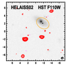
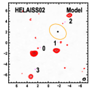
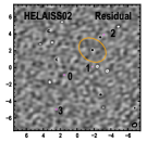
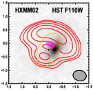
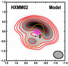
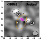
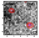
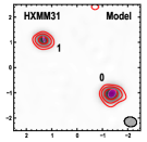
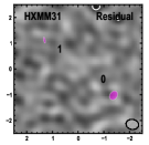
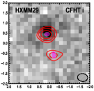
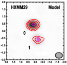
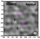
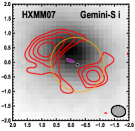
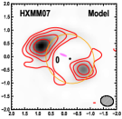
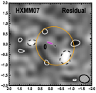
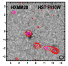
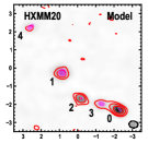
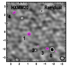
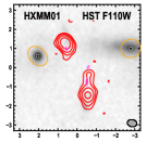
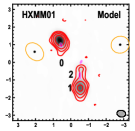
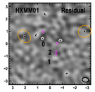
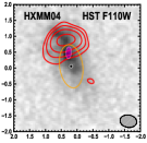
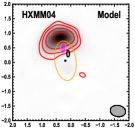
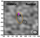
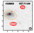
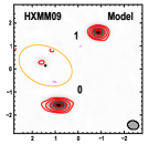
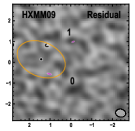
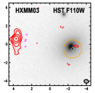
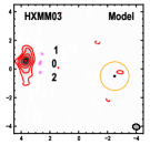
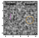
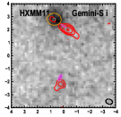
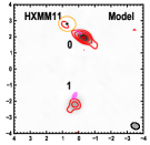
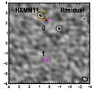
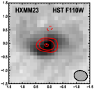
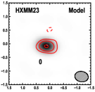
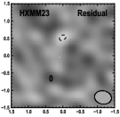
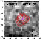
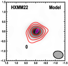
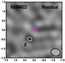
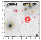
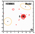
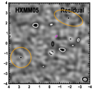
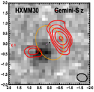
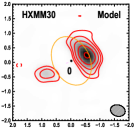
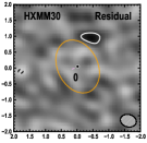
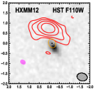
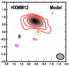
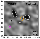
Figure 3.— Model fits for each target in the Herschel-ALMA sample, 3 panels per target. North is up and east is left. Left: ALMA 870$\mu$m imaging (red contours, starting at $\pm 3\sigma$ and increasing by factors of 2) overlaid on best available optical or near-IR imaging (grayscale, with telescope and filter printed in upper right corner). The location and morphology of all sources used in the model are represented by magenta ellipses. If a lens is present, its location is given by a black circle and its critical curve is traced by an orange line. The FWHM size of the ALMA synthesized beam is shown in the lower left corner of each panel. Middle: Same as left, but showing best-fit model in grayscale. Numbers indicate the location of sources. Right: Same as left, but showing residual image obtained from subtracting best-fit model from the data.

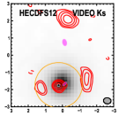
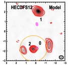
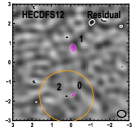
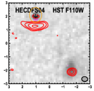
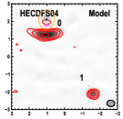
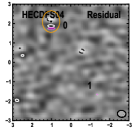
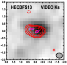
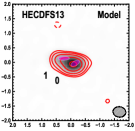
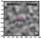
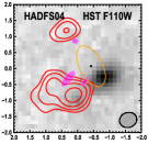
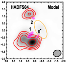
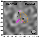
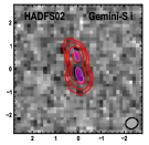
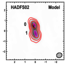
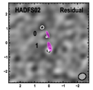
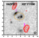
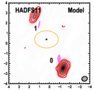
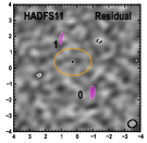
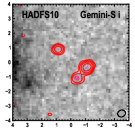
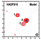
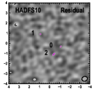
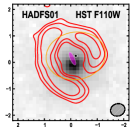
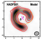
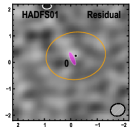
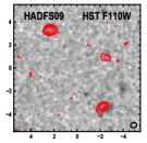
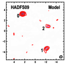
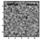
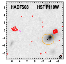
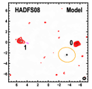
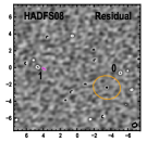
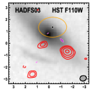
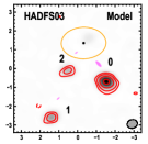
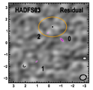
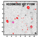
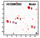
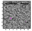
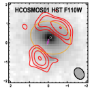
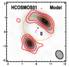
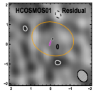
Figure 3.— Continued.

Table 3Intrinsic properties from parameters of model fits to ALMA sources (parameters are described in Section 3.1). Uncertainties in flux densities do not include absolute calibration uncertainty of $\approx 10\%$. Note that some parameters such as source size may become unreliable when the signal to noise ratio is below 10 (e.g., Simpson et al. 2015a).

	$\Delta$RA870	$\Delta$Dec870	$S_{870}$	$r_{\rm s}$		$\phi_{\rm s}$
Short name	($\arcsec$)	($\arcsec$)	(mJy)	($\arcsec$)	$q_{\rm s}$	(deg)	$\mu_{870}$
HELAISS02.0	$3.113\pm 0.160$	$-3.112\pm 0.155$	$8.02\pm 0.15$	$0.096\pm 0.005$	$0.80\pm 0.05$	$91\pm 6$	$1.15\pm 0.07$
HELAISS02.1	$-0.111\pm 0.114$	$-2.172\pm 0.183$	$3.24\pm 0.12$	$0.065\pm 0.008$	$0.84\pm 0.05$	$87\pm 7$	$1.34\pm 0.17$
HELAISS02.2	$-1.470\pm 0.158$	$1.774\pm 0.145$	$3.27\pm 0.25$	$0.105\pm 0.016$	$0.86\pm 0.04$	$120\pm 7$	$1.27\pm 0.13$
HELAISS02.3	$4.039\pm 0.165$	$-7.216\pm 0.174$	$2.22\pm 0.18$	$0.124\pm 0.020$	$0.79\pm 0.05$	$77\pm 7$	$1.08\pm 0.04$
HXMM02.0	$-0.278\pm 0.008$	$0.239\pm 0.011$	$11.88\pm 0.11$	$0.122\pm 0.003$	$0.64\pm 0.02$	$62\pm 2$	$5.33\pm 0.19$
HXMM31.0	$-1.380\pm 0.010$	$-1.025\pm 0.010$	$6.79\pm 0.37$	$0.141\pm 0.011$	$0.80\pm 0.12$	$134\pm 36$	—
HXMM31.1	$1.311\pm 0.011$	$1.124\pm 0.010$	$4.01\pm 0.26$	$0.070\pm 0.018$	$0.59\pm 0.22$	$52\pm 56$	—
HXMM29.0	$0.114\pm 0.009$	$0.451\pm 0.008$	$5.46\pm 0.30$	$0.088\pm 0.012$	$0.82\pm 0.14$	$90\pm 44$	—
HXMM29.1	$-0.236\pm 0.034$	$-0.562\pm 0.030$	$1.82\pm 0.38$	$0.116\pm 0.051$	$0.70\pm 0.20$	$88\pm 55$	—
HXMM07.0	$0.016\pm 0.238$	$-0.016\pm 0.283$	$3.43\pm 0.07$	$0.074\pm 0.007$	$0.32\pm 0.02$	$66\pm 2$	$8.49\pm 1.13$
HXMM20.0	$-2.308\pm 0.012$	$-2.275\pm 0.011$	$7.15\pm 0.44$	$0.089\pm 0.014$	$0.63\pm 0.16$	$58\pm 27$	—
HXMM20.1	$0.828\pm 0.025$	$-0.278\pm 0.023$	$3.52\pm 0.41$	$0.137\pm 0.026$	$0.84\pm 0.10$	$74\pm 44$	—
HXMM20.2	$-0.211\pm 0.017$	$-1.647\pm 0.014$	$3.42\pm 0.26$	$0.058\pm 0.020$	$0.80\pm 0.13$	$84\pm 45$	—
HXMM20.3	$-1.505\pm 0.157$	$-1.981\pm 0.064$	$2.46\pm 0.47$	$0.283\pm 0.198$	$0.67\pm 0.17$	$81\pm 21$	—
HXMM20.4	$2.588\pm 0.155$	$2.611\pm 0.218$	$0.94\pm 0.18$	$0.459\pm 0.246$	$0.58\pm 0.15$	$96\pm 51$	—
HXMM01.0	$-1.503\pm 0.013$	$0.395\pm 0.017$	$11.61\pm 0.23$	$0.090\pm 0.005$	$0.56\pm 0.06$	$12\pm 19$	$1.39\pm 0.19$
HXMM01.1	$-2.563\pm 0.018$	$-1.337\pm 0.017$	$9.56\pm 0.26$	$0.116\pm 0.006$	$0.34\pm 0.03$	$2\pm 1$	$1.21\pm 0.10$
HXMM01.2	$-2.622\pm 0.025$	$-0.552\pm 0.025$	$1.45\pm 0.20$	$0.077\pm 0.025$	$0.66\pm 0.18$	$134\pm 33$	$1.29\pm 0.15$
HXMM04.0	$0.095\pm 0.021$	$0.442\pm 0.025$	$8.49\pm 0.20$	$0.117\pm 0.007$	$0.52\pm 0.07$	$-2\pm 5$	$2.36\pm 0.68$
HXMM09.0	$-0.392\pm 0.039$	$-0.740\pm 0.051$	$5.51\pm 0.19$	$0.064\pm 0.006$	$0.42\pm 0.06$	$75\pm 5$	$1.62\pm 0.31$
HXMM09.1	$-1.507\pm 0.073$	$0.805\pm 0.053$	$5.14\pm 0.15$	$0.033\pm 0.010$	$0.46\pm 0.18$	$116\pm 14$	$1.24\pm 0.12$
HXMM03.0	$5.180\pm 0.003$	$0.924\pm 0.003$	$12.28\pm 0.24$	$0.130\pm 0.004$	$0.53\pm 0.03$	$-25\pm 2$	$1.50\pm 0.25$
HXMM03.1	$7.560\pm 0.023$	$2.051\pm 0.028$	$1.46\pm 0.13$	$0.093\pm 0.007$	$0.73\pm 0.11$	$22\pm 25$	$1.50\pm 0.25$
HXMM03.2	$7.663\pm 0.035$	$0.755\pm 0.033$	$1.35\pm 0.12$	$0.096\pm 0.005$	$0.73\pm 0.11$	$-11\pm 37$	$1.50\pm 0.25$
HXMM11.0	$-0.844\pm 0.111$	$-0.648\pm 0.081$	$6.24\pm 0.24$	$0.106\pm 0.007$	$0.26\pm 0.03$	$54\pm 2$	$1.31\pm 0.16$
HXMM11.1	$-0.596\pm 0.122$	$-4.592\pm 0.098$	$3.38\pm 0.35$	$0.168\pm 0.023$	$0.59\pm 0.16$	$139\pm 41$	$1.05\pm 0.03$
HXMM23.0	$0.101\pm 0.011$	$-0.050\pm 0.009$	$2.93\pm 0.15$	$0.020\pm 0.008$	$0.68\pm 0.20$	$89\pm 49$	—
HXMM22.0	$-0.076\pm 0.004$	$0.024\pm 0.004$	$10.19\pm 0.28$	$0.085\pm 0.010$	$0.52\pm 0.11$	$152\pm 6$	—
HXMM05.0	$-3.505\pm 0.094$	$1.937\pm 0.081$	$12.83\pm 0.31$	$0.095\pm 0.006$	$0.59\pm 0.06$	$142\pm 5$	$1.40\pm 0.20$
HXMM30.0	$0.153\pm 0.024$	$-0.073\pm 0.011$	$0.84\pm 0.01$	$0.019\pm 0.003$	$0.20\pm 0.00$	$109\pm 1$	$27.15\pm 4.61$
HXMM12.0	$1.520\pm 0.168$	$-0.683\pm 0.243$	$9.91\pm 0.24$	$0.115\pm 0.005$	$0.72\pm 0.07$	$69\pm 8$	$1.57\pm 0.29$
HECDFS12.0	$-0.348\pm 0.006$	$0.077\pm 0.004$	$2.02\pm 0.06$	$0.085\pm 0.004$	$0.38\pm 0.03$	$134\pm 3$	$8.29\pm 0.19$
HECDFS12.1	$-0.342\pm 0.005$	$2.489\pm 0.008$	$11.54\pm 0.18$	$0.147\pm 0.003$	$0.65\pm 0.02$	$14\pm 2$	$1.26\pm 0.13$
HECDFS12.2	0.000	0.000	$7.47\pm 0.14$	$0.026\pm 0.009$	$0.79\pm 0.15$	$85\pm 63$	—
HECDFS04.0	$-0.011\pm 0.011$	$-0.347\pm 0.004$	$6.02\pm 0.12$	$0.096\pm 0.005$	$0.35\pm 0.03$	$91\pm 2$	$1.98\pm 0.49$
HECDFS04.1	$-2.366\pm 0.024$	$-3.752\pm 0.007$	$2.51\pm 0.10$	$0.032\pm 0.012$	$0.68\pm 0.19$	$93\pm 55$	$1.06\pm 0.03$
HECDFS13.0	$-0.156\pm 0.011$	$-0.034\pm 0.011$	$10.11\pm 1.30$	$0.099\pm 0.012$	$0.52\pm 0.12$	$123\pm 7$	—
HECDFS13.1	$0.221\pm 0.061$	$0.127\pm 0.018$	$5.25\pm 1.37$	$0.109\pm 0.024$	$0.38\pm 0.08$	$88\pm 7$	—
HADFS04.0	$0.333\pm 0.101$	$-0.513\pm 0.040$	$6.85\pm 0.22$	$0.091\pm 0.006$	$0.39\pm 0.05$	$142\pm 4$	$1.35\pm 0.17$
HADFS04.1	$0.865\pm 0.123$	$-0.420\pm 0.041$	$5.03\pm 0.27$	$0.165\pm 0.013$	$0.43\pm 0.06$	$141\pm 4$	$1.21\pm 0.10$
HADFS04.2	$0.604\pm 0.108$	$0.739\pm 0.077$	$1.99\pm 0.14$	$0.077\pm 0.015$	$0.75\pm 0.16$	$101\pm 40$	$1.40\pm 0.20$
HADFS02.0	$0.067\pm 0.008$	$0.588\pm 0.015$	$7.81\pm 0.47$	$0.136\pm 0.012$	$0.38\pm 0.06$	$23\pm 5$	—
HADFS02.1	$-0.060\pm 0.009$	$-0.268\pm 0.018$	$8.99\pm 0.58$	$0.193\pm 0.015$	$0.42\pm 0.06$	$17\pm 4$	—
HADFS11.0	$-1.340\pm 0.043$	$-1.816\pm 0.119$	$17.51\pm 0.42$	$0.225\pm 0.006$	$0.46\pm 0.02$	$178\pm 1$	$1.21\pm 0.11$
HADFS11.1	$0.658\pm 0.039$	$1.569\pm 0.111$	$5.78\pm 0.24$	$0.180\pm 0.010$	$0.25\pm 0.02$	$167\pm 2$	$1.26\pm 0.13$
HADFS10.0	$-1.126\pm 0.005$	$-0.319\pm 0.004$	$9.61\pm 0.25$	$0.073\pm 0.010$	$0.67\pm 0.15$	$133\pm 24$	—
HADFS10.1	$0.876\pm 0.011$	$0.908\pm 0.009$	$4.59\pm 0.23$	$0.048\pm 0.019$	$0.71\pm 0.19$	$84\pm 43$	—
HADFS10.2	$-0.437\pm 0.017$	$-1.088\pm 0.016$	$3.24\pm 0.19$	$0.093\pm 0.020$	$0.58\pm 0.20$	$131\pm 38$	—
HADFS01.0	$0.131\pm 0.005$	$-0.105\pm 0.006$	$3.17\pm 0.05$	$0.128\pm 0.005$	$0.30\pm 0.01$	$24\pm 1$	$10.34\pm 0.47$
HADFS09.0	$2.343\pm 0.007$	$3.284\pm 0.005$	$8.24\pm 0.26$	$0.109\pm 0.008$	$0.70\pm 0.11$	$92\pm 14$	—
HADFS09.1	$-2.191\pm 0.013$	$-3.320\pm 0.011$	$4.86\pm 0.34$	$0.099\pm 0.019$	$0.53\pm 0.17$	$135\pm 24$	—
HADFS09.2	$-2.503\pm 0.035$	$0.886\pm 0.019$	$2.42\pm 0.35$	$0.122\pm 0.040$	$0.51\pm 0.17$	$89\pm 20$	—
HADFS08.0	$-0.868\pm 0.050$	$0.938\pm 0.048$	$3.74\pm 0.17$	$0.055\pm 0.010$	$0.83\pm 0.09$	$131\pm 20$	$1.65\pm 0.32$
HADFS08.1	$7.496\pm 0.058$	$2.190\pm 0.059$	$7.28\pm 0.39$	$0.179\pm 0.012$	$0.59\pm 0.08$	$63\pm 6$	$1.10\pm 0.05$
HADFS03.0	$-0.734\pm 0.069$	$-1.070\pm 0.053$	$5.39\pm 0.17$	$0.112\pm 0.006$	$0.41\pm 0.05$	$45\pm 3$	$1.32\pm 0.16$
HADFS03.1	$1.415\pm 0.056$	$-2.912\pm 0.059$	$1.87\pm 0.13$	$0.059\pm 0.018$	$0.54\pm 0.12$	$94\pm 48$	$1.13\pm 0.07$
HADFS03.2	$0.427\pm 0.055$	$-0.514\pm 0.059$	$1.22\pm 0.14$	$0.084\pm 0.020$	$0.50\pm 0.13$	$125\pm 14$	$1.86\pm 0.43$
HCOSMOS02.0	$-3.507\pm 0.012$	$4.659\pm 0.013$	$5.26\pm 0.26$	$0.073\pm 0.017$	$0.70\pm 0.12$	$94\pm 34$	—
HCOSMOS02.1	$5.780\pm 0.019$	$-1.434\pm 0.026$	$3.77\pm 0.32$	$0.094\pm 0.029$	$0.76\pm 0.13$	$106\pm 65$	—
HCOSMOS02.2	$-4.869\pm 0.049$	$-3.769\pm 0.050$	$1.69\pm 0.25$	$0.198\pm 0.051$	$0.65\pm 0.13$	$72\pm 41$	—
HCOSMOS02.3	$1.410\pm 0.031$	$-0.035\pm 0.033$	$1.66\pm 0.21$	$0.101\pm 0.042$	$0.71\pm 0.13$	$74\pm 42$	—
HCOSMOS02.4	$3.301\pm 0.083$	$-1.864\pm 0.060$	$2.23\pm 0.41$	$0.312\pm 0.060$	$0.67\pm 0.13$	$78\pm 32$	—
HCOSMOS01.0	$0.136\pm 0.011$	$-0.220\pm 0.016$	$1.03\pm 0.02$	$0.068\pm 0.006$	$0.27\pm 0.04$	$164\pm 2$	$14.86\pm 1.90$

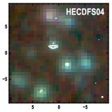
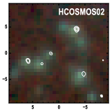
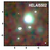
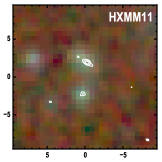
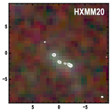
Figure 4.— ALMA 870$\,\mu$m imaging (white contours, starting at 4$\sigma$ and increasing by factors of 2) overlaid on color composite IRAC imaging (blue = 3.6$\,\mu$m, green = 4.5$\,\mu$m, red = 8.0$\,\mu$m). All panels are $27\arcsec$ on a side. North is up and east is left. The synthesized beam is represented in the lower right corner of each panel. Each of the ALMA counterparts are detected in the IRAC imaging. In addition, the IRAC colors of ALMA sources are broadly consistent, providing some evidence that they are at the same redshift and not physically unassociated blends along the line of sight.

4. Results

4.1. De-lensing the ALMA Sample

The combination of our optical or near-IR imaging and our deep, high-resolution ALMA imaging permits us to take the first step towards mapping the foreground structure along the line of sight to the ALMA sources. With such maps in hand for all of our targets, we can estimate the impact that lensing has on the intrinsic properties of the ALMA sources. In other words, we can “de-lens” the Herschel-ALMA sample.

Figure 5 shows the observed (i.e., apparent) and intrinsic (i.e., de-lensed) distributions of $S_{870}$. Lensing has the strongest effect on $S_{870}$: the median flux density in the Herschel-ALMA sample drops by a factor of 1.6 when lensing is taken into account. A two-sided Kolmogorov-Smirnov (KS) test yields a $p$-value of 0.044, suggesting the apparent and intrinsic flux density distributions are inconsistent with being drawn from the same parent population. Even if strongly lensed sources are removed from the sample, the median intrinsic flux density is 1.3 times lower than the median apparent flux density. Removing the unlensed sources from consideration pushes this factor back to 1.6. At these levels, failing to correct for amplification due to gravitational lensing will be a significant source of error, since the absolute calibration uncertainty is typically of order 5-10%. When discussing the intrinsic properties of bright sources (including their number counts, e.g. Wyithe et al. 2011) discovered in wide-field FIR or mm surveys, it is critical to consider the effects of lensing.

For comparison, we also show the cumulative distribution of $S_{870}$ for the ALESS sample (including the completeness limit of LESS of 4.5 mJy). ALESS is the only existing sample of DSFGs with interferometric follow-up of a sensitivity and angular resolution that is comparable to our ALMA data, so it is the best sample with which to compare our results. The significant overlap in $S_{870}$ between our sample and ALESS is evidence that the DSFGs in our sample have higher $S_{500}/S_{870}$ ratios (even when the effect of lensing in our sample is taken into account) than the DSFGs in ALESS (recall Figure 1, which shows that ALESS sources have much lower $S_{500}$ than our targets). This difference is likely due to differences in dust temperature and/or redshift distributions of the two samples and probably arises from selection effects.

The effect on the other source parameters ($r_{\rm s}$, angular separation (the angular distance between an ALMA source and the centroid of all the ALMA sources for a given Herschel DSFG), and $q_{\rm s}$) is less pronounced. The median source size decreases by a factor of 1.2 in the Herschel-ALMA sample after accounting for lensing, but the two-sided KS test reveals a $p$-value of 0.174, suggesting that we cannot rule out the null hypothesis that both size distributions were drawn from the same parent distribution. We find no significant difference between the axial ratios of the apparent and intrinsic distributions, as well as between the angular separations of apparent and intrinsic distributions (two-sided KS test $p$-values of 0.984 and 0.920, respectively).

Finally, the brightest source in the Herschel-ALMA sample is HADFS11.0, with an intrinsic flux density of $S_{870}=17.5\pm 0.4\,$mJy. However, there are also two objects with multiple sources that have separations smaller than 1$\arcsec$, which have summed flux densities comparable to this; namely HADFS02 (16.8 mJy) and HECDFS13 (15.3 mJy). This is approaching the values found in the most extreme systems, such as GN20 (20.6 mJy, Pope et al. 2006) and HFLS3 (15-20 mJy; Riechers et al. 2013; Cooray et al. 2014; Robson et al. 2014). It is a level that is extremely difficult to reproduce in simulations (e.g., Narayanan et al. 2010). One possibility is that the objects with multiple sources represent blends of physically unassociated systems. We explore this possibility via comparison to theoretical models in Section 4.3, but a direct empirical test requires redshift determinations for each source and is beyond the scope of this paper.

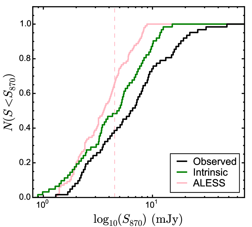
Figure 5.— Cumulative distribution functions showing the effect of lensing on the inferred flux densities of the Herschel-ALMA sample. The median flux density in the Herschel-ALMA sample drops by a factor of 1.3 when lensing is taken into account. For comparison we also show the flux density distribution from ALESS (pink line), with the completeness limit of the LESS survey indicated by a dashed pink line.

4.2. Multiplicity in the ALMA Sample

The second key result from our deep, high-resolution ALMA imaging is a firm measurement of the rate of multiplicity in Herschel DSFGs. We find that 20/29 Herschel DSFGs break down into multiple ALMA sources, implying a multiplicity rate of 69%. However, 5/9 of the single-component systems are strongly lensed. If these five are not considered, then the multiplicity rate increases to 80%. Such a high rate of multiplicity is consistent with theoretical models (e.g., Hayward et al. 2013a, hereafter HB13).

In comparison, the 69 DSFGs in the MAIN ALESS catalog show a multiplicity rate of 35 - 40% (Hodge et al. 2013). Smoothing our ALMA images and adding noise to match the resolution and sensitivity of ALESS results in a multiplicity rate of 55% (four objects with sources that are separated by $<1\arcsec$ become single systems). On the other hand, the ALESS sources are much fainter overall, having a median 870$\,\mu$m flux density of $S_{870}\approx 6\,$mJy, compared to $S_{870}=14.9\,$mJy in our Herschel-ALMA sample. Thus, the evidence favors brighter sources having a higher multiplicity rate. This result is also consistent with multiplicity studies of $S_{870}$-selected DSFGs by Ivison et al. (2007), Smolčić et al. (2012), and Barger et al. (2012), who use VLA, PdBI/1.3 mm, and SMA/870$\,\mu$m imaging to determine rates of 18%, 22%, and 40%, respectively.

One useful way to characterize multiplicity is with a comparison of the total 870$\,\mu$m flux density, $S_{\rm total}$, with the individual component 870$\,\mu$m flux density, $S_{\rm component}$. Figure 6 shows these values for our Herschel-ALMA sample and compares to ALESS. Lensing has a significant impact on the apparent flux densities of many objects in our ALMA sample, so we are careful to show only intrinsic flux densities in this diagram. This diagram reflects the known result that the multipicity rate in ALESS rises and the average fractional contribution per component decreases with increasing $S_{\rm total}$ (Hodge et al. 2013). A simple extrapolation of this phenomenon to the flux density regime probed by our Herschel-ALMA sample would have suggested a very high multiplicity rate and a very low average fractional contribution per component. The multiplicity rate in our sample is indeed higher, but we find that the average fractional contribution per component hovers around 0.4 for essentially the full range in our sample. This is a reflection of the fact that the brightest Herschel DSFGs comprise 1-3 ALMA components, not 5-10 ALMA components as might have been expected from a naive extrapolation of the ALESS results.

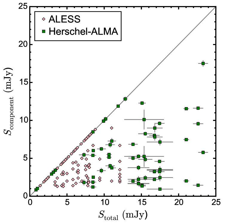
Figure 6.— Comparison of the total 870$\,\mu$m flux density, $S_{\rm total}$, with the individual component 870$\,\mu$m flux density, $S_{\rm component}$ (both of these are after accounting for lensing). Objects falling along the gray dashed line are single component systems (i.e., $S_{\rm total}=S_{\rm component}$). The solid lines trace the average ratio of component to total flux for a given total flux. Our sample of Herschel DSFGs (Herschel-ALMA sample, green squares) has a higher multiplicity and a lower average factional contribution per component than the ALESS sample (pink diamonds), but not as low as would be expected from a simple extrapolation of the trend in the ALESS data alone.

4.3. Spatial Distribution of Multiple Sources

We can dig further into our ALMA data by exploring the average number of ALMA sources per annular area ($dN/dA$) as a function of how far they are from each other. Figure 7 shows the results of this analysis for both our Herschel-ALMA sample and ALESS. We formulate the separation as an angular distance between each ALMA source (using the lensing-corrected data) and the centroid of all of the ALMA sources for that Herschel DSFG. This is different from the pairwise separation distance estimator used by Hodge et al. (2013) that becomes ill-defined when there are more than two ALMA counterparts (as is often the case in our Herschel-ALMA sample). Figure 7 shows $dN/dA$ values for ALESS that have been re-computed using our method. We also show the median and 1$\sigma$ range found from simulated datasets for both ALESS and our Herschel-ALMA sample. The simulated datasets consist of 200 runs of DSFGs with the same flux density and multiplicity as the observed datasets (both the ALESS sample and our ALMA sample), but placed randomly within the primary beam FWHM. We also show predictions from simulations by HB13 (see below for details).

We recover the result from Hodge et al. (2013) that the ALESS DSFGs are consistent with a uniformly distributed population. Interestingly, however, there is a dramatic rise in $dN/dA$ for angular separations less than $2\arcsec$ in our Herschel-ALMA sample. Indeed, for an angular separation of $0\farcs 5$, we find an excess in $dN/dA$ by a factor of $\approx 10$ compared to a random, uniformly distributed population. This excess persists (although at significantly lower amplitude) even when the quality of our ALMA observations are degraded to match the typical sensitivity, spatial resolution, and uv coverage of ALESS (as represented by observations of ALESS 122). The persistence of the excess suggests that it is an intrinsic property of the sample; i.e., that only the brightest DSFGs show an excess of sources on small separation scales (with the caveat that we cannot rule out the possibility of at least part of the excess being due to strong lensing from optically dark lenses).

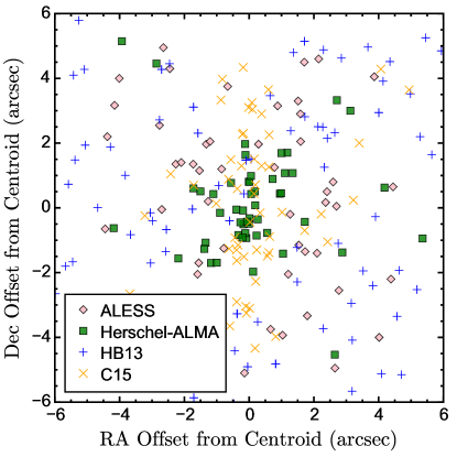
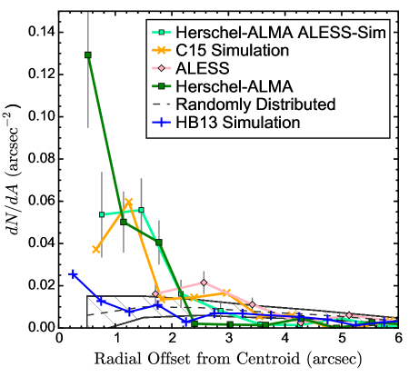
Figure 7.— Left: Spatial distribution of sources with multiple counterparts found in our Herschel-ALMA sample (green squares), in ALESS (pink diamonds) and mock catalogs from HB13 and C15 (blue plus signs and orange crosses, respectively). Sources identified in our Herschel-ALMA sample lie much closer to each other than they do in either ALESS or the HB13 simulations. Right: Number of ALMA sources per annular area as a function of angular separation from the ALMA centroid. Symbols and colors are as in left panel. We also show how our Herschel-ALMA sample would appear if it had been observed with ALESS resolution and sensitivity (light green squares). The range of separations that would be seen if sources were randomly distributed within the ALMA field of view is also shown (dark dashed line and hatched region). The Herschel-ALMA DSFGs show a significantly stronger excess on angular separation scales $<2\arcsec$ compared to both ALESS and the HB13 simulations, even when taking into account the difference in sensitivity and spatial resolution between our ALMA observations and those of ALESS. The simulations from C15 show better agreement with the data, likely due to the more sophisticated treatment of blending compared to HB13.

An excess of sources with small separations from each other could be an indication of interacting or merging systems. However, it is also possible that the sources are merely unrelated galaxies that appear blended due to projection effects (Hayward et al. 2013a; Cowley et al. 2015; Muñoz Arancibia et al. 2015). Spatially resolved spectroscopy is necessary to answer this question definitively, but is not currently available. Instead, to investigate these possibilities further, we make use of mock catalogs of DSFGs that are based on numerical simulations and presented by HB13 and C15.

We begin with the HB13 simulations, summarizing the methodology used to generate the mock catalogs here and refering the reader to HB13 for full details.

Halo catalogs are generated from the Bolshoi dark matter-only cosmological simulation (Klypin et al. 2011) using the rockstar halo finder (Behroozi et al. 2013b, c). Catalogs of subhalos are created from eight randomly chosen lightcones, each with an area of 1.4${}^{\circ}\times 1.4^{\circ}$. Galaxy properties such as stellar mass and SFR are assigned to the subhalos using the abundance matching method of Behroozi et al. (2013a). Dust masses are assigned using an empirically determined redshift-dependent mass–metallicity relation and an assumed dust-to-metal density ratio of 0.4 (see Hayward et al. 2013b for details). Finally, submm flux densities are interpolated from the SFRs and dust masses using a fitting function that is based on the results of dust radiative transfer calculations performed on hydrodynamical simulations of isolated and interacting galaxies (Hayward et al. 2011, 2012b, 2013b).

A blended source is defined as any galaxy in the mock catalogs above a threshold flux density ($S_{\rm thresh}$) that has at least one neighbor within a projected angular distance $d_{\rm neighbor}$. To obtain a direct comparison with our Herschel-ALMA sample, we use $S_{\rm thresh}=1.0\,$mJy (corresponding to the 5$\sigma$ limit of the ALMA data) and $d_{\rm neighbor}=40\arcsec$ (reflecting the size of the Herschel beam at 500$\,\mu$m). We use the known positions in the mock catalogs for all blended sources and compute centroid and separations for every blended source using the same methodology as we applied to our Herschel-ALMA sample and to ALESS.

The $dN/dA$ values found in the mock catalogs are shown by the thick blue line and plus signs in Figure 7. There is a significant increase in $dN/dA$ on separations smaller than $\approx 0\farcs 5$, but the amplitude of the increase is much lower than is apparent in our Herschel-ALMA sample.

The HB13 model does not include SFR enhancements induced by starbursts (see Section 4.5 of Hayward et al. 2013a for a detailed discussion of this limitation). To explore whether interaction-induced starbursts are the origin of the excess at small angular separations observed in our Herschel-ALMA sample, we analyzed modified versions of the HB13 model that include a crude treatment of interaction-induced SFR enhancements (Miller et al. 2015). Mock galaxies with one or more neighbors within a physical distance of 5 kpc and with a stellar mass between one-third and three times that of the galaxy under consideration (i.e. a ‘major merger’) had their SFRs increased by a factor of two. For distances smaller than 1 kpc, the imposed increase was a factor of ten. Because these SFR enhancements are greater than suggested by simulations (e.g. Cox et al. 2008; Hayward et al. 2011, 2014; Torrey et al. 2012) or observations of local galaxy pairs (e.g. Scudder et al. 2012; Patton et al. 2013), we consider this test to provide an upper limit on the possible effect of interactions on blended sources in the HB13 model, although the incompleteness of the Behroozi et al. (2013c) catalogs for mergers with small separations could cause some interacting systems to be missed. We find an insignificant effect on the values of $dN/dA$ when using the merger-induced model as described above. The main reason for this is that only two sources had their SFRs boosted by a factor of ten, and $\approx 150$ experienced a factor of two increase. In the HB13 model, a factor of two increase in SFR corresponds to only a  30% increase in $S_{870}$, so it is perhaps unsurprising that the weak boosts in SFR cause little change in $dN/dA$.

Experiments with stronger interaction-induced SFR enhancements showed that very high enhancements (e.g. a factor of 10 for separation of 5-15 kpc and 100 for separation of $<5\,$kpc) in major mergers are required to match the observed excess in $dN/dA$ on small separations. Incorporating starbursts induced by minor-merger could possibly reduce the required SFR enhancements. The tension between the model prediction and observations may also indicate that a more sophisticated treatment of blending is necessary.

To explore this possibility, we investigate mock catalogs based on the methodology presented in C15. Here, we give a brief summary and refer the interested reader to C15 for full details. A new version of the galform (e.g. Cole et al. 2000, Lacey et al. in preparation) semi-analytic model of hierarchical galaxy formation is used to populate halo merger trees (e.g. Parkinson et al. 2008; Jiang et al. 2014) derived from a Millennium style $N$-body dark matter only simulation (Springel et al. 2005; Guo et al. 2013) with WMAP7 cosmology (Komatsu et al. 2011). A sub-mm flux for each galaxy is calculated using a self-consistent model based on radiative transfer and energy balance arguments. Dust is assumed to exist in two components, dense molecular clouds and a diffuse ISM. Energy absorbed from stellar radiation by each dust component is calculated by solving the equations of radiative transfer in an assumed dust geometry. The dust is then assumed to emit radiation as a modified blackbody.

Three randomly orientated 20 deg² lightcone catalogues are generated using the method described in Merson et al. (2013). We choose as the lower flux limit for inclusion of simulated galaxies into our lightcone catalogue $S_{500\mu\rm{m}}>0.1$ mJy, as this is the limit at which we recover 90% of the extragalactic background light (EBL) as predicted by the model (122 Jy deg^-2). This is in excellent agreement with observations from the COBE satellite (e.g., Puget et al. 1996), and thus ensures a realistic 500 $\mu$m background in the mock images.

Mock imaging is created by binning the lightcone galaxies onto a pixelated grid which is then convolved with a 36$\arcsec$ FWHM Gaussian (corresponding to the Herschel/SPIRE beam at 500$\,\mu$m). The image is then constrained to have a zero mean by the subtraction of a uniform background. No instrumental noise is added, nor are any further filtering procedures applied to the mock image. For the purposes of source identification, this procedure is repeated at 250$\,\mu$m. For this, we adjust the FWHM of the Gaussian PSF to 18$\arcsec$ and change the lower flux limit of inclusion into our lightcone to ensure 90% of the predicted EBL is recovered at this wavelength.

Source positions are selected as maxima in the mock 250$\,\mu$m image, with the position of the source being recorded as the center the maximal pixel for simplicity. To mimic ‘deblended’ Herschel photometry we record the value of the pixel located at the position of the 250$\,\mu$m maxima in the 500$\,\mu$m images. We select all Herschel sources satisfying $S_{500\,\mu\rm{m}}>50\,$mJy and $z>1$ to identify galaxies from our lightcone catalogs within a 9$\arcsec$ radius of the source position, modelling the ALMA primary beam profile as a Gaussian with an 18$\arcsec$ FWHM and a maximum sensitivity of 1 mJy.

The $dN/dA$ values derived from the C15 mock catalogs are shown by the thick orange line and crosses in Figure 7. Here, the amplitude of the increase in $dN/dA$ on separations smaller than $\approx 2\arcsec$ mimics the trend seen in the data. However, there is a deficit of multiple systems with separations of $0\farcs 5$ or less compared to the Herschel-ALMA sample. This result suggests that a sophisticated treatment of blending yields better agreement between simulations and observations but the simulations still under-predict the number of multiple systems with small separations.

Future work on the theoretical side should seek to determine if the application of the C15 blending algorithm to the HB13 simulations yields similarly better agreement with the data. On the observational side, it is critical to establish whether Herschel sources with multiple ALMA counterparts are physically related by measuring spectroscopic redshifts to individual counterparts. Fortunately, this is a viable project today with the VLA and ALMA.

5. Implications for the Bright End of the DSFG Luminosity Function

The distribution of magnification factors for sources found in wide-field surveys with the brightest apparent flux densities are highly sensitive to the shape of the intrinsic number counts at the bright end. In this section, we combine our ALMA and SMA measurements of magnification factors to investigate this as it pertains to DSFGs.

5.1. Statistical Predictions for $\mu_{870}$

Our methodology follows the procedures outlined in previous efforts to predict magnification factors for DSFGs with a given apparent flux density (chiefly, Lima et al. 2010; Wardlow et al. 2013; Fialkov & Loeb 2015). We summarize the essential elements here and highlight significant differences where appropriate.

The key components of the model are the mass density profile of the lenses, $\rho_{\rm lens}\,(r)$, the number density of lenses as a function of mass and redshift, $n_{\rm lens}\,(M,\,z),$ the redshift distribution of the sources, $dN_{\rm source}/dz$, and the intrinsic number counts of the sources, $dn_{\rm source}/dS_{870}^{\prime}$. The latter component is the least certain and also has the strongest impact on the predicted apparent luminosity function. For these reasons, we fix all components of the model except the shape of the intrinsic number counts. Our goal is to take luminosity functions that can successfully fit observed faint DSFG number counts (Karim et al. 2013) and test whether they lead to predicted magnification factors consistent with our ALMA and SMA observations.

To describe $\rho_{\rm lens}\,(r)$, we use a superposition of a singular isothermal sphere (SIS) and a Navarro-Frenk-White (NFW) profile (Navarro et al. 1997) that is truncated at the virial radius. The NFW profile describes the outskirts of dark matter halos better (Mandelbaum et al. 2005), while the SIS profile is preferred on smaller scales because it correctly fits the observed flat rotational curves in galaxies (Kochanek 1994). We make sure that the resulting probability density of lensing, $P\,(\mu)$, is normalized to unity. To describe $n_{\rm lens}\,(M,\,z)$, we generate the abundance of halos at each mass and redshift using the Sheth & Tormen (1999) formalism. To describe $dN_{\rm source}/dz$, we adopt the following redshift distribution which is based on photometric redshifts of optical counterparts to ALMA sources identified in ALESS (Simpson et al. 2014):

$$dN/dz\propto\frac{1}{a_{z}\sigma_{z}\sqrt{2\pi}}\exp\left(\frac{-[\ln(a_{z})-\ln(1+z_{\mu})]^{2}}{2\sigma_{z}^{2}a_{z}}\right),$$ (2)

where $a_{z}=1+z$, $z_{\mu}=1.5$ (to reflect the relatively blue SPIRE colors of the sample), and $\sigma_{z}=0.2$. Alternative values for $z_{\mu}$ and $\sigma_{z}$ yield second-order perturbations which are not significant at the level of our current analysis.

We explore two intrinsic number counts that are intended to bracket the plausible range of values for DSFGs based on two interferometric surveys. One is the number counts measured in ALESS (Karim et al. 2013), and the other is from interferometric follow-up of the first AzTEC survey in COSMOS (Scott et al. 2008) using the SMA (Younger et al. 2007, 2009) and PdBI (Miettinen et al. 2015). These interferometric observations have shown that all of the sources in their surveys are either unlensed or lensed by magnification factors $<2$ (a similar result is found based on ALMA imaging of 52 DSFGs in the Ultra Deep Survey; Simpson et al. 2015a). This is why the ALESS and COSMOS luminosity functions represent a plausible range of intrinsic number counts for DSFGs. These number counts are shown in the left panel of Figure 8. Interferometric follow-up data in COSMOS (Smolčić et al. 2012) and GOODS-N (Barger et al. 2012) are published, but unknown completeness corrections in the single-dish surveys on which these follow-up datasets are based precludes their use here.

In detail, we use a broken power-law of the form

$$\frac{dn}{dS^{\prime}}=N_{\ast}\left(\frac{S^{\prime}}{S_{\ast}}\right)^{-\beta_{1}},~{}~{}~{}~{}\textrm{for}~{}S<S_{\ast},$$ (3)

$$\frac{dn}{dS^{\prime}}=N_{\ast}\left(\frac{S^{\prime}}{S_{\ast}}\right)^{-\beta_{2}},~{}~{}~{}~{}\textrm{for}~{}S>S_{\ast}.$$

Table 4 provides values for the parameters of the broken power-law for the ALESS and COSMOS number counts. The data and corresponding number counts are shown in the left panel of Figure 8.

The product of the model is the lensing optical depth for a given lensing galaxy and source galaxy, $f_{\mu}$. The lensing probability with magnification larger than $\mu$ is then calculated via $P(>\mu)=1-\exp(-f_{\mu})$ and the differential probability distribution is $P(\mu)=-dP(>\mu)/d\mu$. The sum over the distribution of source redshifts and lens masses and redshifts yields the total probability distribution function.

Table 4Parameters of DSFG luminosity functions tested in this paper.

	$N_{\star}$	$S_{\star}$
Luminosity Function	(deg-2)	(mJy)	$\beta_{1}$	$\beta_{2}$
ALESS broken power-law	20	8	2	6.9
COSMOS broken power-law	20	15	2	6.9

The fundamental measurement provided by the spatially resolved ALMA and SMA imaging and associated lens models is the magnification factor of a source with a given apparent $S_{870}$. We use the combined sample to compute the average magnification as a function of $S_{870}$ from the data: $\langle\mu_{870}\rangle$. The same quantity can also be directly computed from our model as

$$\langle\mu_{870}\rangle=\int_{0}^{\infty}\mu P(\mu|S_{870})d\mu,$$ (4)

where the probability for lensing with magnification $\mu$ given the apparent flux is:

$$P(\mu|S_{870})=\frac{1}{N}\frac{P(\mu)}{\mu}\frac{dn}{dS_{870}^{\prime}}\left(\frac{S_{870}}{\mu}\right),$$ (5)

and

$$N=\int\frac{P(\mu)}{\mu}\frac{dn}{dS_{870}^{\prime}}\left(\frac{S_{870}}{\mu}\right)d\mu.$$ (6)

Here $dn/dS_{870}$ is the observed number counts and $dn/dS_{870}^{\prime}$ is the intrinsic number counts.

As part of the lens models, the ALMA and SMA imaging also provide the probability that a source with a given apparent $S_{870}$ experiences a magnification above some threshold value, $\mu_{\rm min}$: $P\,(\mu>\mu_{\rm min})$. It is therefore of interest to make a similar prediction from our model. We use the following to do this:

$$P(\mu>\mu_{\rm min})=\frac{\int_{\mu}^{\infty}P(\mu|S_{obs})}{\int_{0}^{\infty}P(\mu|S_{obs})}.$$ (7)

5.2. Comparing Models with Data

The middle panel of Figure 8 shows a direct comparison of the measured $\mu_{870}$ values as a function of apparent $S_{870}$ for the Herschel-ALMA and Herschel-SMA samples. We also show a running average of the combined sample (considering only $\mu_{870}>2.0$ objects) to serve as a direct comparison to our theoretical models. We compute this by interpolating the observed $\mu_{870}$ and $S_{870}$ onto a fine grid using the Scipy griddata package and then smoothing the resulting grid using a Gaussian filter in the Scipy gaussian_filter package. Also shown in this diagram are model predictions for the average magnification as a function of $S_{870}$, $\langle\mu_{870}\rangle$, assuming the two intrinsic number counts for DSFGs described in Table 4.

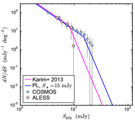
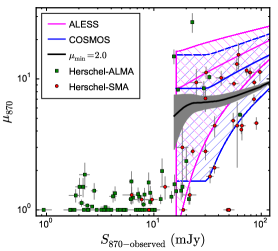
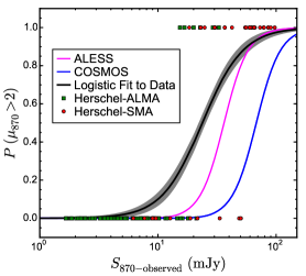
Figure 8.— Left: Observed number counts from interferometer follow-up of mm sources in COSMOS (black circles; Younger et al. 2007, 2009; Miettinen et al. 2015) and from ALESS (pink diamonds; Karim et al. 2013). The magneta and blue lines represent the range of plausible intrinsic number counts for DSFGs given these two datasets. Middle: Magnification factors at 870$\,\mu$m as a function of apparent $S_{870}$ for every source in our ALMA (green squares) and SMA (red circles) samples. The black line represents a running average of the magnification measurements when sources with $\mu_{870}>2.0$ are considered (grey shaded region highlights the 1$\sigma$ uncertainty), and is truncated at the minimum flux density at which we have observed $\mu_{870}>2.0$. Colored lines show the average magnification factor, $\langle\mu_{870}\rangle$, predicted by our models for the two intrinsic number counts shown on the left. The model number counts predict higher $\langle\mu_{870}\rangle$ than are seen in the data. Right: Probability that a source with a given $S_{870}$ experiences $\mu_{870}>2.0$. The black line (grey shaded region) shows a logistic regression fit to the SMA and ALMA data (grey shaded region highlights the 1$\sigma$ uncertainty). Colored lines are the same as in the middle and left panels. The intrinsic number counts that provide a good fit to the COSMOS data predict too many unlensed or weakly lensed sources with intrinsic flux densities of $S_{870}^{\prime}\sim 50\,$mJy.

Both models predict higher $\langle\mu_{870}\rangle$ than are seen in the data by factors of 5-10. However, the dispersion in the predicted $\langle\mu_{870}\rangle$ values for both intrinsic number counts rises smoothly from $\sigma_{\mu}\approx 2$ at $S_{870}=15\,$mJy to $\sigma_{\mu}\approx 8$ at $S_{870}=100\,$mJy, so this difference is not statistically significant. Furthermore, there is reason to believe that the data may be biased against high magnification factor measurements. In both the Herschel-ALMA and Herschel-SMA samples, the spatial resolution is $\approx 0\farcs 5$. This is nearly always sufficient to resolve the images of the lensed galaxy, but it is not always sufficient to resolve the images themselves. Therefore, it may be the case that the lens models over-predict the intrinsic sizes of the lensed galaxies and hence under-predict the magnification factors. For example, the average half-light sizes of unlensed DSFGs have been found recently to be $\approx 0.8\,$kpc (Ikarashi et al. 2014) and $\approx 1.2\,$kpc (Simpson et al. 2015a). In contrast, we reported a median half-light radius of $1.53\,$kpc in Bussmann et al. (2013). Lens models from higher resolution data with ALMA suggest that magnification factors could increase by a factor of $\approx 1.5-2$ (Rybak et al. 2015; Tamura et al. 2015; Dye et al. 2015). Therefore, it is plausible that both of the intrinsic luminosity functions tested here provide statistically consistent fits to the data.

A related but distinct test of the intrinsic number counts for DSFGs comes from the probability of a given source experiencing a magnification above some threshold value, $\mu_{\rm min}$. Unlike the case with the average magnification factor measurements, our ALMA and SMA data should provide a reliable estimate of this quantity. The results of this are shown in the right panel of Figure 8. For clarity of presentation, we show one choice of $\mu_{\rm min}$: $\mu_{\rm min}=2.0$. The shape of the curves varies with $\mu_{\rm min}$, but the overall results are qualitatively the same. The models we consider are the same as those used in the left panel of Figure 8. Instead of computing a running average of the data, we show a logistic regression fit to the data (obtained with the Scikit-learn package; Pedregosa et al. 2011).

Both models tested in this paper exhibit a sharp transition from low probability to high probability of being lensed, consistent with the data. However, there are significant differences in where this transition flux density, $S_{\rm trans}$, occurs — i.e., where $P(\mu>\mu_{870})>2$. In the data, the logistic regression fit yields $S_{\rm trans}=24\pm 3\,$mJy (error accounts only for statistical uncertainty in $S_{870}$ and $\mu_{870}$), whereas the models based on the ALESS and COSMOS number counts yield $S_{\rm trans}=37\,$mJy $S_{\rm trans}=69\,$mJy, respectively.

This analysis highlights the difficulty encountered with the luminosity function based on the COSMOS data: unlensed sources with $S_{870}>50\,$mJy are over-predicted and lensed sources with $S_{870}<50\,$mJy are under-predicted. If the ALESS number counts continue to be supported by the evidence as additional data are obtained (e.g.; Simpson et al. 2015b), the implications are significant. We should then expect to find $\approx 3$ sources satisfying $S_{870}>10\,$mJy in a 1 deg² survey. This is about a factor of 7 lower than typical measurements from single-dish, broad-beam studies (e.g., Weiß et al. 2009). This suggests that very luminous galaxies such as GN20 and HFLS3 may be more rare than previously thought.

6. Conclusions

We present ALMA 870$\,\mu$m $0\farcs 45$ imaging of 29 Herschel DSFGs selected from 55 deg² of HerMES. The Herschel sources have $S_{500}=52-134\,$mJy, placing them in a unique phase space between the brightest sources found by Herschel and those found in ground-based surveys at sub-mm wavelengths that include more typical, fainter galaxies. Our ALMA observations reveal 62 sources down to the 5$\sigma$ limit ($\sigma\approx 0.3\,$mJy, typically). We make use of optical and near-IR imaging to assess the distribution of intervening galaxies along the line of sight. We introduce a new, publicly available software called uvmcmcfit and use it to develop lens models for all ALMA sources with nearby foreground galaxy. Our results from this effort are summarized as follows:

1. 36/62 ALMA sources experience significant amplification from a nearby foreground galaxy that is comparable to or greater than the absolute calibration uncertainty (i.e., $\mu_{870}>1.1$). The median amplification in the subset that experiences lensing is $\mu_{870}=1.6$. Only 6 sources show morphology typical of strong gravitational lensing and could be identified as lenses from the ALMA imaging alone. A multi-wavelength approach is critical to identifying structure along the line of sight and determining an unbiased measurement of the flux densities in our sample.

2. 20/29 Herschel DSFGs break down into multiple ALMA counterparts. Of the 9 isolated systems, 5 are strongly lensed by factors of 5-30 (HECDFS12 is a non-isolated system with a strongly lensed source in it). After correcting for amplification, the brightest source in the sample has $S_{870}=17.5\pm 0.4\,$mJy. There is a weak trend towards even higher multiplicity at the highest total $S_{870}$ flux densities.

3. When a Herschel source comprises multiple ALMA counterparts, these counterparts are typically located within 2$\arcsec$ of each other. Their separations are significantly smaller than ALMA counterparts to ALESS sources as well as simulated sources from HB13 and C15, although the improved treatment of blending by the latter yields superior agreement with the data. This conclusion remains true even when we degrade our ALMA observations to match the spatial resolution, sensitivity, and uv coverage of the ALESS observations.

4. Intrinsic number counts for DSFGs with a form that matches observations in COSMOS (Miettinen et al. 2015) under-predict the number of lensed sources with apparent $S_{870}>10\,$mJy. Number counts based on ALESS observations provide a better match to our magnification measurements. The interpretation of these results is complicated by the fact that our sample is likely biased towards blends of multiple sources within a Herschel beam. Our primary goal is to draw attention to this analysis method as a means to test number counts of DSFGs using wide-field Herschel data.

If the ALESS number counts continue to provide the best predicted magnification factors in larger samples with weaker biases, this suggests that galaxies with intrinsic flux densities above $S_{870}^{\prime}\approx 10\,$mJy are extremely rare. One possible explanation for their rarity is that they are simply the tip of the mass function among starbursts. An alternative is that they represent a very short phase in galaxy evolution. It is interesting to note that consistent with this idea is the high multiplicity rate in our ALMA sample as well as the small projected separations between multiple ALMA counterparts. The inability of numerical simulations to reproduce the small projected separations seen in the data might highlight a productive path forward to improve our theoretical understanding of the enhancement in star-formation by interactions and mergers of galaxies which are already forming stars at a very high rate.

In the future, higher spatial resolution imaging is needed to investigate the morphologies of individual ALMA sources. Tidal tails, multiple nuclei, and other signs of mergers and interactions should become evident at $0\farcs 1$ resolution. In addition, molecular spectroscopy will be critical to determine distances to and dynamics of individual ALMA sources and hence characterize what fraction of Herschel sources are actually physically associated with each other (and not simply a result of projection effects along the line of sight). Finally, deeper optical or near-IR imaging is needed to search for dark lenses that may have been missed in our Gemini-S or HST imaging.

Appendix A Herschel/SPIRE Photometry

We present in Table 5 SPIRE photometry ($S_{250}$, $S_{350}$, and $S_{500}$) for each Herschel source in our sample using as priors the ALMA and Spitzer 24$\,\mu$m counterpart positions. Many of the Herschel sources in our sample have multiple 24$\,\mu$m counterparts close enough to the ALMA counterparts that they can make a significant contribution to the SPIRE flux at the position of the ALMA counterparts. For this reason, it is critical to include the 24$\,\mu$m data when estimating Herschel/SPIRE photometry. In cases where the Spitzer 24$\,\mu$m and ALMA counterparts spatially overlap (defined here as having a separation smaller than $2\farcs 5$), we exclude the Spitzer counterpart from the calculations.

Note that in the case of HELAISS02, we exclude a 24$\,\mu$m source associated with the lensing galaxy, despite being more than $2\farcs 5$ away from the nearest ALMA counterpart. This is because the ALMA counterparts are arranged so that they surround the 24$\mu$m source completely. The extended emission seen in the SPIRE maps is therefore most likely attributable to the ALMA counterparts rather than the 24$\,\mu$m source.

One of the key results from this analysis is that the use of StarFinder to deconvolve the SPIRE beam will lead to the removal of a portion of the targets with extended emission from a flux-limited sample. This is by design, as the goal outlined in Wardlow et al. (2013) was to develop the purest sample of lens candidates as possible from HerMES data. Blends were considered by these authors to be unlikely to be lensed. This method is effective for lenses where the Einstein radius is smaller than $\approx 2\arcsec$. However, it selects against deeper potential wells, such as those of groups or clusters (e.g., HLock01 Gavazzi et al. 2011), that produce images separated by scales that comprise a significant fraction of the SPIRE PSF.

It is worth emphasizing that blends likely constitute an interesting path of study for future work, as they potentially represent proto-groups or proto-clusters during a particular active stage of their evolution. They are also prime examples of systems of sources that are poorly reproduced in simulations, as evidenced by the investigations in Section 4.3 in this paper. Table 5 shows that one possible means of selecting candidate blends is by comparing the SUSSEXtractor and StarFinder flux densities, particularly at 500$\,\mu$m. A large difference between these two measurements likely indicates multiple components separated by scales that are a significant fraction of the SPIRE beam (e.g., HELAISS02, HXMM20, and HCOSMOS02).

Table 5Compilation of Herschel/SPIRE flux density measurements. For each Herschel source, we give the fiducial flux densities (denoted in table as “Fiducial”), the initial flux densities obtained using SUSSEXtractor that were then used to generate the target list for the ALMA observations (“SUSSEXtractor”), and the flux densities obtained subsequently using the more sophisticated deblending algorithm from StarFinder that were then used to construct the list of lens candidates presented in Wardlow et al. (2013) (“StarFinder”). In all cases, uncertainties are comparable to the uncertainties given in Table 1.

	Fiducial			StarFinder			SUSSEXtractor
	$S_{250}$	$S_{350}$	$S_{500}$	$S_{250}$	$S_{350}$	$S_{500}$	$S_{250}$	$S_{350}$	$S_{500}$
Short name	(mJy)	(mJy)	(mJy)	(mJy)	(mJy)	(mJy)	(mJy)	(mJy)	(mJy)
HELAISS02	115	124	108	114	101	76	105	128	103
HXMM02	78	122	99	92	122	113	101	147	141
HXMM31	102	94	65	128	112	73	129	116	80
HXMM29	97	102	78	89	83	56	100	107	80
HXMM07	89	107	85	91	104	86	92	104	83
HXMM20	72	85	66	85	79	67	80	96	88
HXMM01	179	188	134	180	192	132	178	195	137
HXMM04	162	157	125	144	137	94	173	174	127
HXMM09	129	118	85	120	115	84	135	113	95
HXMM03	114	134	116	121	132	110	118	137	118
HXMM11	101	104	73	107	108	81	105	121	94
HXMM23	128	105	68	137	108	57	132	118	88
HXMM22	101	85	61	97	82	62	147	128	89
HXMM05	103	118	97	106	119	92	103	115	101
HXMM30	86	97	75	90	100	75	93	105	80
HXMM12	98	106	82	102	110	81	107	115	89
HECDFS12	61	82	81	28	84	85	68	92	100
HECDFS04	56	61	55	73	86	85	65	87	96
HECDFS13	95	89	63	96	90	63	88	85	51
HADFS04	74	93	84	76	90	72	71	95	87
HADFS02	102	97	81	110	102	87	103	100	79
HADFS11	19	39	52	57	78	75	57	87	97
HADFS10	47	58	58	96	86	57	121	114	76
HADFS01	76	100	94	80	103	93	72	108	87
HADFS09	98	102	72	115	61	24	112	117	86
HADFS08	142	133	90	88	81	50	126	130	102
HADFS03	119	102	63	138	114	73	134	124	86
HCOSMOS02	70	85	71	71	64	41	82	99	89
HCOSMOS01	86	96	71	91	100	74	89	99	73

References

- Aravena et al. (2010) Aravena, M., Bertoldi, F., Carilli, C., Schinnerer, E., McCracken, H. J., Salvato, M., Riechers, D., Sheth, K., Smǒlcić, V., Capak, P., Koekemoer, A. M., & Menten, K. M. 2010, ApJ, 708, L36
- Barger et al. (2012) Barger, A. J., Wang, W.-H., Cowie, L. L., Owen, F. N., Chen, C.-C., & Williams, J. P. 2012, ApJ, 761, 89
- Behroozi et al. (2013a) Behroozi, P. S., Wechsler, R. H., & Conroy, C. 2013a, ApJ, 770, 57
- Behroozi et al. (2013b) Behroozi, P. S., Wechsler, R. H., & Wu, H.-Y. 2013b, ApJ, 762, 109
- Behroozi et al. (2013c) Behroozi, P. S., Wechsler, R. H., Wu, H.-Y., Busha, M. T., Klypin, A. A., & Primack, J. R. 2013c, ApJ, 763, 18
- Blain (1996) Blain, A. W. 1996, MNRAS, 283, 1340
- Bothwell et al. (2013) Bothwell, M. S., Smail, I., Chapman, S. C., Genzel, R., Ivison, R. J., Tacconi, L. J., Alaghband-Zadeh, S., Bertoldi, F., Blain, A. W., Casey, C. M., Cox, P., Greve, T. R., Lutz, D., Neri, R., Omont, A., & Swinbank, A. M. 2013, MNRAS, 429, 3047
- Bussmann et al. (2012) Bussmann, R. S., Gurwell, M. A., Fu, H., Smith, D. J. B., Dye, S., Auld, R., Baes, M., Baker, A. J., Bonfield, D., Cava, A., Clements, D. L., Cooray, A., Coppin, K., Dannerbauer, H., Dariush, A., De Zotti, G., Dunne, L., Eales, S., Fritz, J., Hopwood, R., Ibar, E., Ivison, R. J., Jarvis, M. J., Kim, S., Leeuw, L. L., Maddox, S., Michałowski, M. J., Negrello, M., Pascale, E., Pohlen, M., Riechers, D. A., Rigby, E., Scott, D., Temi, P., Van der Werf, P. P., Wardlow, J., Wilner, D., & Verma, A. 2012, ApJ, 756
- Bussmann et al. (2013) Bussmann, R. S., Pérez-Fournon, I., Amber, S., Calanog, J., Gurwell, M. A., Dannerbauer, H., De Bernardis, F., Fu, H., Harris, A. I., Krips, M., Lapi, A., Maiolino, R., Omont, A., Riechers, D., Wardlow, J., Baker, A. J., Birkinshaw, M., Bock, J., Bourne, N., Clements, D. L., Cooray, A., De Zotti, G., Dunne, L., Dye, S., Eales, S., Farrah, D., Gavazzi, R., González Nuevo, J., Hopwood, R., Ibar, E., Ivison, R. J., Laporte, N., Maddox, S., Martínez-Navajas, P., Michalowski, M., Negrello, M., Oliver, S. J., Roseboom, I. G., Scott, D., Serjeant, S., Smith, A. J., Smith, M., Streblyanska, A., Valiante, E., van der Werf, P., Verma, A., Vieira, J. D., Wang, L., & Wilner, D. 2013, ApJ, 779, 25
- Calanog et al. (2014) Calanog, J. A., Fu, H., Cooray, A., Wardlow, J., Ma, B., Amber, S., Baes, M., Bock, J., Bourne, N., Bussmann, R. S., Casey, C. M., Chapman, S. C., Clements, D. L., Conley, A., Dannerbauer, H., DeZotti, G., Dunne, L., Dye, S., Eales, S., Farrah, D., Furlanetto, C., Harris, A. I., Ivison, R. J., Maddox, S. J., Magdis, G., Michalowski, M. J., Negrello, M., Nightingale, J., O’Bryan, J. M., Oliver, S. J., Riechers, D., Scott, D., Serjeant, S., Simpson, J., Smith, M., Timmons, N., Thacker, C., Valiante, E., & Vieira, J. D. 2014, ArXiv e-prints
- Capak et al. (2011) Capak, P. L., Riechers, D., Scoville, N. Z., Carilli, C., Cox, P., Neri, R., Robertson, B., Salvato, M., Schinnerer, E., Yan, L., Wilson, G. W., Yun, M., Civano, F., Elvis, M., Karim, A., Mobasher, B., & Staguhn, J. G. 2011, Nature, 470, 233
- Carlstrom et al. (2011) Carlstrom, J. E. et al. 2011, PASP, 123, 568
- Casey et al. (2012a) Casey, C. M., Berta, S., Béthermin, M., Bock, J., Bridge, C., Budynkiewicz, J., Burgarella, D., Chapin, E., Chapman, S. C., Clements, D. L., Conley, A., Conselice, C. J., Cooray, A., Farrah, D., Hatziminaoglou, E., Ivison, R. J., le Floc’h, E., Lutz, D., Magdis, G., Magnelli, B., Oliver, S. J., Page, M. J., Pozzi, F., Rigopoulou, D., Riguccini, L., Roseboom, I. G., Sanders, D. B., Scott, D., Seymour, N., Valtchanov, I., Vieira, J. D., Viero, M., & Wardlow, J. 2012a, ApJ, 761, 140
- Casey et al. (2012b) Casey, C. M., Berta, S., Béthermin, M., Bock, J., Bridge, C., Burgarella, D., Chapin, E., Chapman, S. C., Clements, D. L., Conley, A., Conselice, C. J., Cooray, A., Farrah, D., Hatziminaoglou, E., Ivison, R. J., le Floc’h, E., Lutz, D., Magdis, G., Magnelli, B., Oliver, S. J., Page, M. J., Pozzi, F., Rigopoulou, D., Riguccini, L., Roseboom, I. G., Sanders, D. B., Scott, D., Seymour, N., Valtchanov, I., Vieira, J. D., Viero, M., & Wardlow, J. 2012b, ApJ, 761, 139
- Casey et al. (2014) Casey, C. M., Narayanan, D., & Cooray, A. 2014, Phys. Rep., 541, 45
- Chapman et al. (2005) Chapman, S. C., Blain, A. W., Smail, I., & Ivison, R. J. 2005, ApJ, 622, 772
- Cole et al. (2000) Cole, S., Lacey, C. G., Baugh, C. M., & Frenk, C. S. 2000, MNRAS, 319, 168
- Condon et al. (1998) Condon, J. J., Cotton, W. D., Greisen, E. W., Yin, Q. F., Perley, R. A., Taylor, G. B., & Broderick, J. J. 1998, AJ, 115, 1693
- Conley et al. (2011) Conley, A. et al. 2011, ApJ, 732, L35
- Cooray et al. (2014) Cooray, A., Calanog, J., Wardlow, J. L., Bock, J., Bridge, C., Burgarella, D., Bussmann, R. S., Casey, C. M., Clements, D., Conley, A., Farrah, D., Fu, H., Gavazzi, R., Ivison, R. J., La Porte, N., Lo Faro, B., Ma, B., Magdis, G., Oliver, S. J., Osage, W. A., Pérez-Fournon, I., Riechers, D., Rigopoulou, D., Scott, D., Viero, M., & Watson, D. 2014, ApJ, 790, 40
- Cowley et al. (2015) Cowley, W. I., Lacey, C. G., Baugh, C. M., & Cole, S. 2015, MNRAS, 446, 1784
- Cox et al. (2008) Cox, T. J., Jonsson, P., Somerville, R. S., Primack, J. R., & Dekel, A. 2008, MNRAS, 384, 386
- Daddi et al. (2009) Daddi, E. et al. 2009, ApJ, 694, 1517
- Dye et al. (2015) Dye, S., Furlanetto, C., Swinbank, A. M., Vlahakis, C., Nightingale, J. W., Dunne, L., Eales, S. A., Smail, I., Oteo-Gomez, I., Hunter, T., Negrello, M., Dannerbauer, H., Ivison, R. J., Gavazzi, R., Cooray, A., & van der Werf, P. 2015, ArXiv e-prints
- Eales et al. (2010) Eales, S. et al. 2010, PASP, 122, 499
- Engel et al. (2010) Engel, H., Tacconi, L. J., Davies, R. I., Neri, R., Smail, I., Chapman, S. C., Genzel, R., Cox, P., Greve, T. R., Ivison, R. J., Blain, A., Bertoldi, F., & Omont, A. 2010, ApJ, 724, 233
- Fialkov & Loeb (2015) Fialkov, A. & Loeb, A. 2015, ArXiv e-prints
- Foreman-Mackey et al. (2013) Foreman-Mackey, D., Hogg, D. W., Lang, D., & Goodman, J. 2013, PASP, 125, 306
- Fu et al. (2013) Fu, H. et al. 2013, Nature, 498, 338
- Gavazzi et al. (2011) Gavazzi, R. et al. 2011, ApJ, 738, 125
- Goodman & Weare (2010) Goodman, J. & Weare, J. 2010, Communications in Applied Mathematics and Computational Science, 5, 65
- Griffin et al. (2010) Griffin, M. J. et al. 2010, A&A, 518, L3+
- Guo et al. (2013) Guo, Q., White, S., Angulo, R. E., Henriques, B., Lemson, G., Boylan-Kolchin, M., Thomas, P., & Short, C. 2013, MNRAS, 428, 1351
- Hayward et al. (2013a) Hayward, C. C., Behroozi, P. S., Somerville, R. S., Primack, J. R., Moreno, J., & Wechsler, R. H. 2013a, MNRAS
- Hayward et al. (2012a) Hayward, C. C., Jonsson, P., Kereš, D., Magnelli, B., Hernquist, L., & Cox, T. J. 2012a, MNRAS, 424, 951
- Hayward et al. (2012b) —. 2012b, MNRAS, 424, 951
- Hayward et al. (2011) Hayward, C. C., Kereš, D., Jonsson, P., Narayanan, D., Cox, T. J., & Hernquist, L. 2011, ApJ, 743, 159
- Hayward et al. (2013b) Hayward, C. C., Narayanan, D., Kereš, D., Jonsson, P., Hopkins, P. F., Cox, T. J., & Hernquist, L. 2013b, MNRAS, 428, 2529
- Hayward et al. (2014) Hayward, C. C., Torrey, P., Springel, V., Hernquist, L., & Vogelsberger, M. 2014, MNRAS, 442, 1992
- Hezaveh et al. (2013) Hezaveh, Y. D. et al. 2013, ApJ, 767, 132
- Hinshaw et al. (2013) Hinshaw, G., Larson, D., Komatsu, E., Spergel, D. N., Bennett, C. L., Dunkley, J., Nolta, M. R., Halpern, M., Hill, R. S., Odegard, N., Page, L., Smith, K. M., Weiland, J. L., Gold, B., Jarosik, N., Kogut, A., Limon, M., Meyer, S. S., Tucker, G. S., Wollack, E., & Wright, E. L. 2013, ApJS, 208, 19
- Ho et al. (2004) Ho, P. T. P., Moran, J. M., & Lo, K. Y. 2004, ApJ, 616, L1
- Hodge et al. (2013) Hodge, J. A. et al. 2013, ApJ, 768, 91
- Hook et al. (2004) Hook, I. M., Jørgensen, I., Allington-Smith, J. R., Davies, R. L., Metcalfe, N., Murowinski, R. G., & Crampton, D. 2004, PASP, 116, 425
- Ikarashi et al. (2014) Ikarashi, S., Ivison, R. J., Caputi, K. I., Aretxaga, I., Dunlop, J. S., Hatsukade, B., Hughes, D., Iono, D., Izumi, T., Kawabe, R., Kohno, K., Lagos, C. P., Motohara, K., Nakanishi, K., Ohta, K., Tamura, Y., Umehata, H., Wilson, G., Yabe, K., & Yun, M. S. 2014, ArXiv e-prints
- Ikarashi et al. (2011) Ikarashi, S. et al. 2011, MNRAS, 415, 3081
- Ivison et al. (2007) Ivison, R. J., Greve, T. R., Dunlop, J. S., Peacock, J. A., Egami, E., Smail, I., Ibar, E., van Kampen, E., Aretxaga, I., Babbedge, T., Biggs, A. D., Blain, A. W., Chapman, S. C., Clements, D. L., Coppin, K., Farrah, D., Halpern, M., Hughes, D. H., Jarvis, M. J., Jenness, T., Jones, J. R., Mortier, A. M. J., Oliver, S., Papovich, C., Pérez-González, P. G., Pope, A., Rawlings, S., Rieke, G. H., Rowan-Robinson, M., Savage, R. S., Scott, D., Seigar, M., Serjeant, S., Simpson, C., Stevens, J. A., Vaccari, M., Wagg, J., & Willott, C. J. 2007, MNRAS, 380, 199
- Ivison et al. (2011) Ivison, R. J., Papadopoulos, P. P., Smail, I., Greve, T. R., Thomson, A. P., Xilouris, E. M., & Chapman, S. C. 2011, MNRAS, 412, 1913
- Ivison et al. (2013) Ivison, R. J. et al. 2013, ApJ, 772, 137
- Jarvis et al. (2013) Jarvis, M. J., Bonfield, D. G., Bruce, V. A., Geach, J. E., McAlpine, K., McLure, R. J., González-Solares, E., Irwin, M., Lewis, J., Yoldas, A. K., Andreon, S., Cross, N. J. G., Emerson, J. P., Dalton, G., Dunlop, J. S., Hodgkin, S. T., Le, F. O., Karouzos, M., Meisenheimer, K., Oliver, S., Rawlings, S., Simpson, C., Smail, I., Smith, D. J. B., Sullivan, M., Sutherland, W., White, S. V., & Zwart, J. T. L. 2013, MNRAS, 428, 1281
- Jiang et al. (2014) Jiang, L., Helly, J. C., Cole, S., & Frenk, C. S. 2014, MNRAS, 440, 2115
- Karim et al. (2013) Karim, A. et al. 2013, MNRAS, 432, 2
- Keeton (2001) Keeton, C. R. 2001, ArXiv Astrophysics e-prints
- Klypin et al. (2011) Klypin, A. A., Trujillo-Gomez, S., & Primack, J. 2011, ApJ, 740, 102
- Kochanek (1994) Kochanek, C. S. 1994, ApJ, 436, 56
- Komatsu et al. (2011) Komatsu, E., Smith, K. M., Dunkley, J., Bennett, C. L., Gold, B., Hinshaw, G., Jarosik, N., Larson, D., Nolta, M. R., Page, L., Spergel, D. N., Halpern, M., Hill, R. S., Kogut, A., Limon, M., Meyer, S. S., Odegard, N., Tucker, G. S., Weiland, J. L., Wollack, E., & Wright, E. L. 2011, ApJS, 192, 18
- Lilly et al. (1996) Lilly, S. J., Le Fevre, O., Hammer, F., & Crampton, D. 1996, ApJ, 460, L1
- Lima et al. (2010) Lima, M., Jain, B., & Devlin, M. 2010, MNRAS, 406, 2352
- Madau et al. (1996) Madau, P., Ferguson, H. C., Dickinson, M. E., Giavalisco, M., Steidel, C. C., & Fruchter, A. 1996, MNRAS, 283, 1388
- Magnelli et al. (2011) Magnelli, B., Elbaz, D., Chary, R. R., Dickinson, M., Le Borgne, D., Frayer, D. T., & Willmer, C. N. A. 2011, A&A, 528, A35+
- Mandelbaum et al. (2005) Mandelbaum, R., Tasitsiomi, A., Seljak, U., Kravtsov, A. V., & Wechsler, R. H. 2005, MNRAS, 362, 1451
- Merson et al. (2013) Merson, A. I., Baugh, C. M., Helly, J. C., Gonzalez-Perez, V., Cole, S., Bielby, R., Norberg, P., Frenk, C. S., Benson, A. J., Bower, R. G., Lacey, C. G., & Lagos, C. d. P. 2013, MNRAS, 429, 556
- Messias et al. (2014) Messias, H., Dye, S., Nagar, N., Orellana, G., Bussmann, R. S., Calanog, J., Dannerbauer, H., Fu, H., Ibar, E., Inohara, A., Ivison, R. J., Negrello, M., Riechers, D. A., Sheen, Y.-K., Aguirre, J. E., Amber, S., Birkinshaw, M., Bourne, N., Bradford, C. M., Clements, D. L., Cooray, A., De Zotti, G., Demarco, R., Dunne, L., Eales, S., Fleuren, S., Kamenetzky, J., Lupu, R. E., Maddox, S. J., Marrone, D. P., Michałowski, M. J., Murphy, E. J., Nguyen, H. T., Omont, A., Rowlands, K., Smith, D., Smith, M., Valiante, E., & Vieira, J. D. 2014, A&A, 568, A92
- Miettinen et al. (2015) Miettinen, O., Smolčić, V., Novak, M., Aravena, M., Karim, A., Masters, D., Riechers, D. A., Bussmann, R. S., McCracken, H. J., Ilbert, O., Bertoldi, F., Capak, P., Feruglio, C., Halliday, C., Kartaltepe, J. S., Navarrete, F., Salvato, M., Sanders, D., Schinnerer, E., & Sheth, K. 2015, ArXiv e-prints
- Miller et al. (2015) Miller, T. B., Hayward, C. C., Chapman, S. C., & Behroozi, P. S. 2015, ArXiv e-prints
- Muñoz Arancibia et al. (2015) Muñoz Arancibia, A. M., Navarrete, F. P., Padilla, N. D., Cora, S. A., Gawiser, E., Kurczynski, P., & Ruiz, A. N. 2015, MNRAS, 446, 2291
- Narayanan et al. (2010) Narayanan, D., Hayward, C. C., Cox, T. J., Hernquist, L., Jonsson, P., Younger, J. D., & Groves, B. 2010, MNRAS, 401, 1613
- Navarro et al. (1997) Navarro, J. F., Frenk, C. S., & White, S. D. M. 1997, ApJ, 490, 493
- Negrello et al. (2007) Negrello, M., Perrotta, F., González-Nuevo, J., Silva, L., de Zotti, G., Granato, G. L., Baccigalupi, C., & Danese, L. 2007, MNRAS, 377, 1557
- Negrello et al. (2010) Negrello, M. et al. 2010, Science, 330, 800
- Nguyen et al. (2010) Nguyen, H. T. et al. 2010, A&A, 518, L5
- Oliver et al. (2012) Oliver, S. J. et al. 2012, MNRAS, 424, 1614
- Parkinson et al. (2008) Parkinson, H., Cole, S., & Helly, J. 2008, MNRAS, 383, 557
- Patton et al. (2013) Patton, D. R., Torrey, P., Ellison, S. L., Mendel, J. T., & Scudder, J. M. 2013, MNRAS, 433, L59
- Pedregosa et al. (2011) Pedregosa, F. et al. 2011, Journal of Machine Learning Research, 12, 2825
- Pilbratt et al. (2010) Pilbratt, G. L. et al. 2010, A&A, 518, L1
- Pope et al. (2006) Pope, A. et al. 2006, MNRAS, 370, 1185
- Puget et al. (1996) Puget, J.-L., Abergel, A., Bernard, J.-P., Boulanger, F., Burton, W. B., Desert, F.-X., & Hartmann, D. 1996, A&A, 308, L5
- Riechers et al. (2011a) Riechers, D. A. et al. 2011a, ApJ, 733, L12
- Riechers et al. (2011b) —. 2011b, ApJ, 733, L11+
- Riechers et al. (2013) —. 2013, Nature, 496, 329
- Rieke et al. (2004) Rieke, G. H. et al. 2004, ApJS, 154, 25
- Robson et al. (2014) Robson, E. I., Ivison, R. J., Smail, I., Holland, W. S., Geach, J. E., Gibb, A. G., Riechers, D., Ade, P. A. R., Bintley, D., Bock, J., Chapin, E. L., Chapman, S. C., Clements, D. L., Conley, A., Cooray, A., Dunlop, J. S., Farrah, D., Fich, M., Fu, H., Jenness, T., Laporte, N., Oliver, S. J., Omont, A., Pérez-Fournon, I., Scott, D., Swinbank, A. M., & Wardlow, J. 2014, ApJ, 793, 11
- Rybak et al. (2015) Rybak, M., McKean, J. P., Vegetti, S., Andreani, P., & White, S. D. M. 2015, ArXiv e-prints
- Savage & Oliver (2007) Savage, R. S. & Oliver, S. 2007, ApJ, 661, 1339
- Scott et al. (2008) Scott, K. S., Austermann, J. E., Perera, T. A., Wilson, G. W., Aretxaga, I., Bock, J. J., Hughes, D. H., Kang, Y., Kim, S., Mauskopf, P. D., Sanders, D. B., Scoville, N., & Yun, M. S. 2008, MNRAS, 385, 2225
- Scudder et al. (2012) Scudder, J. M., Ellison, S. L., Torrey, P., Patton, D. R., & Mendel, J. T. 2012, MNRAS, 426, 549
- Sersic (1968) Sersic, J. L. 1968, Atlas de galaxias australes (Cordoba, Argentina: Observatorio Astronomico, 1968)
- Sheth & Tormen (1999) Sheth, R. K. & Tormen, G. 1999, MNRAS, 308, 119
- Simpson et al. (2015a) Simpson, J. M., Smail, I., Swinbank, A. M., Almaini, O., Blain, A. W., Bremer, M. N., Chapman, S. C., Chen, C.-C., Conselice, C., Coppin, K. E. K., Danielson, A. L. R., Dunlop, J. S., Edge, A. C., Farrah, D., Geach, J. E., Hartley, W. G., Ivison, R. J., Karim, A., Lani, C., Ma, C.-J., Meijerink, R., Michałowski, M. J., Mortlock, A., Scott, D., Simpson, C. J., Spaans, M., Thomson, A. P., van Kampen, E., & van der Werf, P. P. 2015a, ApJ, 799, 81
- Simpson et al. (2015b) Simpson, J. M., Smail, I., Swinbank, A. M., Chapman, S. C., Geach, J. E., Ivison, R. J., Thomson, A. P., Aretxaga, I., Blain, A. W., Cowley, W. I., Chen, C.-C., Coppin, K. E. K., Dunlop, J. S., Edge, A. C., Farrah, D., Ibar, E., Karim, A., Knudsen, K. K., Meijerink, R., Michałowski, M. J., Scott, D., Spaans, M., & van der Werf, P. P. 2015b, ApJ, 807, 128
- Simpson et al. (2014) Simpson, J. M., Swinbank, A. M., Smail, I., Alexander, D. M., Brandt, W. N., Bertoldi, F., de Breuck, C., Chapman, S. C., Coppin, K. E. K., da Cunha, E., Danielson, A. L. R., Dannerbauer, H., Greve, T. R., Hodge, J. A., Ivison, R. J., Karim, A., Knudsen, K. K., Poggianti, B. M., Schinnerer, E., Thomson, A. P., Walter, F., Wardlow, J. L., Weiß, A., & van der Werf, P. P. 2014, ApJ, 788, 125
- Smith et al. (2012) Smith, A. J., Wang, L., Oliver, S. J., Auld, R., Bock, J., Brisbin, D., Burgarella, D., Chanial, P., Chapin, E., Clements, D. L., Conversi, L., Cooray, A., Dowell, C. D., Eales, S., Farrah, D., Franceschini, A., Glenn, J., Griffin, M., Ivison, R. J., Mortier, A. M. J., Page, M. J., Papageorgiou, A., Pearson, C. P., Pérez-Fournon, I., Pohlen, M., Rawlings, J. I., Raymond, G., Rodighiero, G., Roseboom, I. G., Rowan-Robinson, M., Savage, R., Scott, D., Seymour, N., Symeonidis, M., Tugwell, K. E., Vaccari, M., Valtchanov, I., Vigroux, L., Ward, R., Wright, G., & Zemcov, M. 2012, MNRAS, 419, 377
- Smolčić et al. (2012) Smolčić, V., Aravena, M., Navarrete, F., Schinnerer, E., Riechers, D. A., Bertoldi, F., Feruglio, C., Finoguenov, A., Salvato, M., Sargent, M., McCracken, H. J., Albrecht, M., Karim, A., Capak, P., Carilli, C. L., Cappelluti, N., Elvis, M., Ilbert, O., Kartaltepe, J., Lilly, S., Sanders, D., Sheth, K., Scoville, N. Z., & Taniguchi, Y. 2012, A&A, 548, A4
- Springel et al. (2005) Springel, V., White, S. D. M., Jenkins, A., Frenk, C. S., Yoshida, N., Gao, L., Navarro, J., Thacker, R., Croton, D., Helly, J., Peacock, J. A., Cole, S., Thomas, P., Couchman, H., Evrard, A., Colberg, J., & Pearce, F. 2005, Nature, 435, 629
- Swetz et al. (2011) Swetz, D. S. et al. 2011, ApJS, 194, 41
- Swinbank et al. (2014) Swinbank, A. M., Simpson, J. M., Smail, I., Harrison, C. M., Hodge, J. A., Karim, A., Walter, F., Alexander, D. M., Brandt, W. N., de Breuck, C., da Cunha, E., Chapman, S. C., Coppin, K. E. K., Danielson, A. L. R., Dannerbauer, H., Decarli, R., Greve, T. R., Ivison, R. J., Knudsen, K. K., Lagos, C. D. P., Schinnerer, E., Thomson, A. P., Wardlow, J. L., Weiß, A., & van der Werf, P. 2014, MNRAS, 438, 1267
- Tacconi et al. (2008) Tacconi, L. J. et al. 2008, ApJ, 680, 246
- Tamura et al. (2015) Tamura, Y., Oguri, M., Iono, D., Hatsukade, B., Matsuda, Y., & Hayashi, M. 2015, ArXiv e-prints
- Torrey et al. (2012) Torrey, P., Cox, T. J., Kewley, L., & Hernquist, L. 2012, ApJ, 746, 108
- Treu (2010) Treu, T. 2010, ARA&A, 48, 87
- Vieira et al. (2013) Vieira, J. D. et al. 2013, Nature, 495, 344
- Wang et al. (2014) Wang, L., Viero, M., Clarke, C., Bock, J., Buat, V., Conley, A., Farrah, D., Guo, K., Heinis, S., Magdis, G., Marchetti, L., Marsden, G., Norberg, P., Oliver, S. J., Page, M. J., Roehlly, Y., Roseboom, I. G., Schulz, B., Smith, A. J., Vaccari, M., & Zemcov, M. 2014, MNRAS, 444, 2870
- Wardlow et al. (2013) Wardlow, J. L. et al. 2013, ApJ, 762, 59
- Weiß et al. (2009) Weiß, A., Kovács, A., Coppin, K., Greve, T. R., Walter, F., Smail, I., Dunlop, J. S., Knudsen, K. K., Alexander, D. M., Bertoldi, F., Brandt, W. N., Chapman, S. C., Cox, P., Dannerbauer, H., De Breuck, C., Gawiser, E., Ivison, R. J., Lutz, D., Menten, K. M., Koekemoer, A. M., Kreysa, E., Kurczynski, P., Rix, H.-W., Schinnerer, E., & van der Werf, P. P. 2009, ApJ, 707, 1201
- Wyithe et al. (2011) Wyithe, J. S. B., Yan, H., Windhorst, R. A., & Mao, S. 2011, Nature, 469, 181
- Younger et al. (2007) Younger, J. D., Fazio, G. G., Huang, J.-S., Yun, M. S., Wilson, G. W., Ashby, M. L. N., Gurwell, M. A., Lai, K., Peck, A. B., Petitpas, G. R., Wilner, D. J., Iono, D., Kohno, K., Kawabe, R., Hughes, D. H., Aretxaga, I., Webb, T., Martínez-Sansigre, A., Kim, S., Scott, K. S., Austermann, J., Perera, T., Lowenthal, J. D., Schinnerer, E., & Smolčić, V. 2007, ApJ, 671, 1531
- Younger et al. (2009) Younger, J. D., Fazio, G. G., Huang, J.-S., Yun, M. S., Wilson, G. W., Ashby, M. L. N., Gurwell, M. A., Peck, A. B., Petitpas, G. R., Wilner, D. J., Hughes, D. H., Aretxaga, I., Kim, S., Scott, K. S., Austermann, J., Perera, T., & Lowenthal, J. D. 2009, ApJ, 704, 803