On the intrinsic bottom content of the nucleon and its impact on heavy new physics at the LHC

Abstract

Heavy quark parton distribution functions (PDFs) play an important role in several Standard Model and New Physics processes. Most analyses rely on the assumption that the charm and bottom PDFs are generated perturbatively by gluon splitting and do not involve any non-perturbative degrees of freedom. It is clearly necessary to test this hypothesis with suitable QCD processes. Conversely, a non-perturbative, intrinsic heavy quark parton distribution has been predicted in the literature. We demonstrate that to a very good approximation the scale-evolution of the intrinsic heavy quark content of the nucleon is governed by non-singlet evolution equations. This allows us to analyze the intrinsic heavy quark distributions without having to resort to a full-fledged global analysis of parton distribution functions. We exploit this freedom to model intrinsic bottom distributions which are so far missing in the literature in order to estimate the impact of this non-perturbative contribution to the bottom-quark PDF, and on parton–parton luminosities at the LHC. This technique can be applied to the case of intrinsic charm, albeit within the limitations outlined in the following.

1 Introduction

Heavy quark parton distribution functions (PDFs) play an important role in several Standard Model (SM) and New Physics (NP) processes at the CERN Large Hadron Collider (LHC). In particular, several key processes involve the bottom quark PDF, e.g. $tW$, $tH^{+}$ production, associated $b$ plus $W/Z/H$ boson production or $Hbb$ production Maltoni:2012pa . In the standard approach employed by almost all global analyses of PDFs, the heavy quark distributions are generated radiatively, according to DGLAP evolution equations Altarelli:1977zs ; Gribov:1972ri ; Dokshitzer:1977sg , starting with a perturbatively calculable boundary condition Collins:1986mp ; Buza:1996wv at a scale of the order of the heavy quark mass. In other words, there are no free fit parameters associated with the heavy quark distribution and it is entirely related to the gluon PDF at the scale of the boundary condition. As a consequence, the uncertainties for the heavy quark and gluon distributions are strongly correlated; this has been discussed in the context of inclusive Higgs production at the Tevatron and LHC Belyaev:2005nu .

However, a purely perturbative, extrinsic, treatment where the heavy quarks are radiatively generated might not be adequate; in particular for the charm quark with a mass $m_{c}\simeq 1.3$ GeV which is not much bigger than typical hadronic scales but also for the bottom quark with a mass $m_{b}\simeq 4.5$ GeV. Indeed, there are a number of models that postulate a non-perturbative, intrinsic, heavy quark component which is present even for scales $Q$ below the heavy quark mass $m$. In particular, light-cone models predict a non-perturbative (’intrinsic’) heavy quark component in the proton wave-function Brodsky:1980pb ; Brodsky:1981se and similar expectations result from meson cloud models Navarra:1995rq ; Paiva:1996dd ; Melnitchouk:1997ig ; an overview of different models can be found, e.g., in Pumplin:2005yf . Predictions of these models together with the EMC charm data Aubert:1982tt ; Aubert:1981ix motivated first theoretical analyses of the intrinsic charm (IC) content of the proton Hoffmann:1983ah ; Harris:1995jx ; Steffens:1999hx . These first analyses were not global as they concentrated only on the possibility of explaining the EMC data. Later the CTEQ collaboration performed the first fully global analyses of PDFs including the IC possibility Pumplin:2007wg ; Nadolsky:2008zw . These studies gave the first estimate, based on an array of different data sets, of how big the intrinsic charm could be. The possibility of IC was also considered by the MSTW group Martin:2009iq . Most recently, two new global PDF analyses dedicated to IC have been performed: (i) the CTEQ collaboration has updated their previous work Dulat:2013hea using the CT10 NNLO framework Gao:2013xoa , and (ii) an analysis of Jimenez-Delgado et al. Jimenez-Delgado:2014zga which is interesting as it uses less strict kinematic cuts which allow for the inclusion of low-$Q$, high-$x$ data that should be more sensitive to the light-cone inspired IC component. These two most recent analyses set significantly different limits on the allowed IC contribution, partly because of the very different tolerance criteria which are used to define the range of acceptable fits. These differences highlight the utility of the techniques discussed in this paper as we can freely adjust the amount of IC/IB contributions (within limits, which we will quantify) without having to regenerate a complete global analysis for each case.

It is essential to experimentally test the heavy quark PDFs, both the extrinsic and intrinsic components. One observable which is directly sensitive to an IC component is the deep inelastic charm structure function $F_{2}^{c}(x,Q^{2})$. So far, the EMC data for $F_{2}^{c}$ is the only measurement of the charm structure function in the relevant $(x,Q^{2})$ region which is sensitive to a large-$x$ IC component; this is the only DIS data cited as evidence for intrinsic charm. The HERA data on $F_{2}^{c}$ and $F_{2}^{b}$ exist only for $x<0.1$ and provide no constraints on a large-$x$ IC or IB; only the inclusive structure function $F_{2}(x,Q^{2})$ at large-$x$ measured quite precisely at HERA provides limited information on the large-$x$ charm PDF. At a future Electron-Ion Collider (EIC) the large-$x$ charm structure function would be accessible, and the rate for charm production at $x\gtrsim 0.1$ could be increased by up to an order of magnitude due to the presence of a large-$x$ non-perturbative intrinsic charm component in the nucleon Boer:2011fh . Alternatively, the IC could be searched for by measuring the Callan-Gross ratio $R(x,Q^{2})=F_{L}/F_{T}$ Ivanov:2008xu , or by studying angular distributions Ananikyan:2007ef ; Ananikyan:2006kz .

In hadronic collisions, a promising way to constrain models of IC is the measurement of inclusive charm hadron production ($D^{0},D^{+},D^{\star+},\Lambda_{c},\ldots$). Predictions for such processes were obtained in the general-mass variable-flavor-number scheme (GM-VFNS) Kniehl:2004fy ; Kniehl:2005mk ; Kniehl:2005st for the Tevatron at a center-of-mass (cms) energy of 1960 GeV, for the Relativistic Heavy Ion Collider (RHIC) at cms energies of 200 GeV (RHIC200) and 500 GeV (RHIC500), and for the LHC at a cms energy of 7 TeV (LHC7) Spiesberger:2012zn ; Kniehl:2012ti ; Kniehl:2011bk ; Kniehl:2009ar . The IC charm effects can be particularly large at the RHIC200 and at the LHC7 at forward rapidities where the differential cross section can be enhanced by a factor of up to 5 compared to the prediction with a radiatively generated charm PDF Kniehl:2012ti . Recent results from LHCb Aaij:2013mga can serve as an example of such data which are, however, not yet precise enough and do not extend to sufficiently large transverse momenta at the most forward rapidities ($4<y<4.5$) to be conclusive. Another process which is very sensitive to the heavy quark PDF is direct photon production in association with a heavy quark jet Kovarik:2012pj . Data from the D0 experiment at the Tevatron Abazov:2009de ; Abazov:2012ea overshoot the standard NLO QCD predictions Stavreva:2009vi at large transverse photon momenta; the inclusion of an intrinsic heavy quark component in the nucleon can reduce the difference between data and theory, but not fully resolve it. In fact, at the Tevatron the $q\bar{q}$ channel becomes important at large transverse momenta, and higher-order corrections to this channel not included in Ref. Stavreva:2009vi might explain (part of) this discrepancy. The $q\bar{q}$-channel does not play an important role at $pp$ colliders; therefore, measurements of this process at RHIC and the LHC probe the heavy quark PDFs in different regions of the momentum fraction $x$ and could shed more light on the current situation. A detailed study of $\gamma+Q$ production at the LHC operating at $\sqrt{S}=8$ TeV (LHC8) was performed in Refs. Bednyakov:2014pqa ; Bednyakov:2013zta . There it was shown that the existence of IC in the proton can be visible at large transverse momenta of the photons and heavy quark jets at rapidities $1.5<|y_{\gamma}|<2.4,|y_{c}|<2.4$. Indeed, for the BHPS model Brodsky:1980pb the cross section can be enhanced by a factor of 2 or 3 for $p_{T}^{\gamma}>200$ GeV. However, the cross section is already quite small in this kinematic range so that this measurement will be statistically limited. The ideal place to observe or constrain intrinsic charm would be A Fixed Target ExpeRiment using the LHC beams (AFTER and LHC) Brodsky:2012vg ; Lansberg:2012kf ; Lansberg:2013wpx ; Rakotozafindrabe:2013cmt due to the lower cms energy ($\sqrt{S}=115$ GeV) together with a very high luminosity; for a review see review_ic .

While there are at least a few global analyses which allow for an intrinsic charm component in the nucleon Pumplin:2007wg ; Nadolsky:2008zw ; Dulat:2013hea ; Jimenez-Delgado:2014zga , studies of intrinsic bottom PDFs have not been performed at all. The main purpose of this paper is to outline a technique which can provide IB PDFs for any generic non-IB PDF set; we can then directly compare the IB PDFs with the non-IB PDFs to gauge the impact of the non-perturbative IB component of the nucleon structure on $b$-quark initiated processes. Our approach exploits the fact that the intrinsic bottom PDF evolves (to an excellent precision) according to a standalone non-singlet evolution equation. Furthermore, due to the small momentum fraction carried by the IB PDF, the evolution of the other partons is essentially not disturbed by the IB component. These two observation allows us to compute the IB PDF without the need to perform a complete global analysis of PDFs. Thus, we can easily obtain a matched set of IB and non-IB PDFs. Note that because existing data entering global analyses of proton PDFs do not constrain the IB PDF, it would not be useful to try and obtain information on the IB content of the nucleon using a global fit.

The rest of this paper is organized as follows. In Sec. 2, we demonstrate that the scale-evolution of the intrinsic PDF is governed by a non-singlet evolution equation. We then propose suitable boundary conditions and perform a number of numerical tests of the quality of our approximations. In particular, we investigate to what degree the gluon distribution is perturbed by the presence of the intrinsic component. In Sec. 3, we use the IB PDFs to obtain predictions for parton–parton luminosities relevant at the LHC. In Sec. 4, we discuss our results and assess the impact of the intrinsic component. Finally, in Sec. 5, we summarize our results and present conclusions.

2 Intrinsic heavy quark PDFs

2.1 Definition

In the context of a global analysis of PDFs the different parton flavors are specified via a boundary condition at the input scale $\mu_{0}$ which is typically of the order ${\cal O}(1\ {\rm GeV})$. Solving the DGLAP evolution equations with these boundary conditions allows us to determine the PDFs at higher scales $\mu>\mu_{0}$. The boundary conditions for the up, down, strange quarks and gluons are not perturbatively calculable and have to be determined from experimental data. From this perspective, it is meaningless to decompose the light quark and gluons PDFs into distinct (extrinsic and intrinsic) components. The situation is different for the heavy charm and bottom quarks; the boundary conditions have been calculated perturbatively and resum to all orders collinear logarithms associated with the heavy quark lines at fixed-order in perturbation theory. A non-perturbative (intrinsic) heavy quark distribution $Q_{1}$ can then be defined at the input scale $\mu_{0}$ as the difference of the full boundary condition for the heavy quark PDF $Q$ and the perturbatively calculable (extrinsic) boundary condition $Q_{0}$:

$$Q_{1}(x,\mu_{0}):=Q(x,\mu_{0})-Q_{0}(x,\mu_{0})\,,$$ (1)

where $Q=c$ or $Q=b$. At NLO in the ${\rm{\overline{MS}}}$ scheme, the relation in Eq. (1) gets further simplified if the input scale $\mu_{0}$ is identified with the heavy quark mass $m_{Q}$ because $Q_{0}(x,m_{Q})=0$ at NLO. In this case, any non-zero boundary condition $Q(x,m_{Q})\neq 0$ can be attributed to the intrinsic heavy quark component. This simplification, however, does not hold a priori for a different factorization scheme, nor at NNLO and beyond.

2.2 Evolution

In the following, we demonstrate that to a good approximation the intrinsic heavy quark distributions are governed by non-singlet evolution equations. Denoting the vector of light quarks as ‘$q$’ and the heavy quark distribution by ‘$Q$’ (where $Q=c$ or $Q=b$) the Dokshitzer-Gribov-Lipatov-Altarelli-Parisi (DGLAP) evolution equations read Altarelli:1977zs ; Gribov:1972ri ; Dokshitzer:1977sg

$$\dot{g} = P_{gg}\otimes g+P_{gq}\otimes q+P_{gQ}\otimes Q\,,$$ (2)

$$\dot{q} = P_{qg}\otimes g+P_{qq}\otimes q+P_{qQ}\otimes Q\,,$$ (3)

$$\dot{Q} = P_{Qg}\otimes g+P_{Qq}\otimes q+P_{QQ}\otimes Q\,,$$ (4)

with the splitting functions $P_{Qg}(x)=P_{qg}(x)$, $P_{QQ}(x)=P_{qq}(x)$, $P_{Qq}(x)=P_{q^{\prime}q}(x)$, etc. in the massless ${\rm{\overline{MS}}}$ scheme which are known up to three-loop order Vogt:2004mw ; Moch:2004pa .

Next we substitute $Q=Q_{0}+Q_{1}$ where $Q_{0}$ denotes the usual radiatively generated extrinsic heavy quark component and $Q_{1}$ is the non-perturbative intrinsic heavy quark distribution:

$$\dot{g} = P_{gg}\otimes g+P_{gq}\otimes q+P_{gQ}\otimes Q_{0}+{\cancel{P_{gQ}\otimes Q_{1}}}\,,$$ (5)

$$\dot{q} = P_{qg}\otimes g+P_{qq}\otimes q+P_{qQ}\otimes Q_{0}+{\cancel{P_{qQ}\otimes Q_{1}}}\,,$$ (6)

$$\dot{Q}_{0}+\dot{Q}_{1} = P_{Qg}\otimes g+P_{Qq}\otimes q+P_{QQ}\otimes Q_{0}+P_{QQ}\otimes Q_{1}\,.$$ (7)

Neglecting the crossed out terms which give a tiny contribution to the evolution of the gluon and light quark distributions the system of evolution equations can be separated into two independent parts. For the system of gluon, light quarks and extrinsic heavy quark ($g,q,Q_{0}$) one recovers the same evolution equations as in the standard approach without an intrinsic heavy quark component

$$\dot{g} = P_{gg}\otimes g+P_{gq}\otimes q+P_{gQ}\otimes Q_{0}\,,$$ (8)

$$\dot{q} = P_{qg}\otimes g+P_{qq}\otimes q+P_{qQ}\otimes Q_{0}\,,$$ (9)

$$\dot{Q}_{0} = P_{Qg}\otimes g+P_{Qq}\otimes q+P_{QQ}\otimes Q_{0}\,.$$ (10)

For the intrinsic heavy quark distribution, $Q_{1}$, one finds a standalone non-singlet evolution equation

$$\dot{Q}_{1}=P_{QQ}\otimes Q_{1}\,.$$ (11)

In a global analysis with intrinsic heavy quark PDFs, using the exact evolution equations (2)–(4), the parton distributions satisfy the momentum sum rule

$$\int_{0}^{1}\ {\operatorname{d}}x\ x\ \left(g+\sum_{i}(q_{i}+\bar{q}_{i})+Q_{0}+\bar{Q}_{0}+Q_{1}+\bar{Q}_{1}\right)=1\,.$$ (12)

Allowing for a small violation of this sum rule it is possible to entirely decouple the analysis of the intrinsic heavy quark distribution from the rest of the system. The PDFs for the gluon, the light quarks and the extrinsic heavy quark can be taken from a global analysis in the standard approach using Eqs. (8) – (10) where they already saturate the momentum sum rule

$$\int_{0}^{1}\ {\operatorname{d}}x\ x\ \left(g+\sum_{i}(q_{i}+\bar{q}_{i})+Q_{0}+\bar{Q}_{0}\right)=1\,.$$ (13)

On top of these PDFs the intrinsic heavy quark PDF can be determined in a standalone analysis using the non-singlet evolution equation (11). This induces a violation of the momentum sum rule by the term

$$\int_{0}^{1}\ {\operatorname{d}}x\ x\ \left(Q_{1}+\bar{Q}_{1}\right)$$ (14)

which, however, is very small for bottom quarks. We will perform numerical checks of the validity of our approximations in Sec. 2.5 after having discussed the boundary conditions for the intrinsic heavy quark distribution.

2.3 Modeling the boundary condition

The BHPS model Brodsky:1980pb predicts the following $x$-dependence for the intrinsic charm (IC) parton distribution function:

$$c_{1}(x)=\bar{c}_{1}(x)\propto x^{2}[6x(1+x)\ln x+(1-x)(1+10x+x^{2})]\,.$$ (15)

Conversely, the normalization and the precise energy scale of this distribution are not specified. In the CTEQ global analyses with intrinsic charm Pumplin:2007wg ; Nadolsky:2008zw this functional form has been used as a boundary condition at the scale $Q=m_{c}$ leaving the normalization as a free fit parameter.

We expect the $x$-shape of the intrinsic bottom distribution $b_{1}(x)$ to be very similar to the one of the intrinsic charm distribution. Furthermore, the normalization of IB is expected to be parametrically suppressed with respect to IC by a factor $m_{c}^{2}/m_{b}^{2}\simeq 0.1$. Therefore, because the scale of the boundary condition is not fixed, the following two ansatzes for $b_{1}$ can be considered

$${\rm\it Different\ Scales:}\qquad b_{1}(x,m_{b})=\frac{m_{c}^{2}}{m_{b}^{2}}\,c_{1}(x,m_{c})\,,$$ (16)

$${\rm\it Same\ Scales:}\qquad b_{1}(x,m_{c})=\frac{m_{c}^{2}}{m_{b}^{2}}c_{1}(x,m_{c})\,.$$ (17)

In the following we use the Same Scales boundary condition, Eq. (17), which remains valid at any scale $Q$.

In this case, since $c_{1}=c-c_{0}$, it is possible to construct the IB PDF from the difference of the CTEQ6.6c and the standard CTEQ6.6 charm PDFs at any scale without having to solve the non-singlet evolution equation for the IB PDF. We will compare the two boundary conditions in Eqs. (16) and (17) in Sec. 2.5. Finally, let us note that it would be no problem to work with asymmetric boundary conditions, $\bar{c}_{1}(x)\neq c_{1}(x)$ and $\bar{b}_{1}(x)\neq b_{1}(x)$, as predicted for example by meson cloud models Paiva:1996dd .

2.4 Intrinsic heavy quark PDFs from non-singlet evolution

For the purpose of this analysis we used the approximation of Sec. 2.2 to produce standalone IC and IB PDFs that can be used together with any regular PDF set sharing the same values for the QCD parameters, such as the strong coupling or the quark masses. For the IC PDF we used Eq. (15) to define the initial $x$-dependence at the scale of the charm mass, and fixed the normalization to match the one predicted by the CTEQ6.6c0 fit Nadolsky:2008zw . The IB PDF was generated using the Same Scales boundary conditions of Eq. (17) together with the same $x$-dependent input of Eq. (15). If not stated otherwise, the normalization for the IB PDF was chosen to be identical to the IC case scaled down by a factor $m_{c}^{2}/m_{b}^{2}=0.083$. Both PDFs were then evolved according to the non-singlet evolution equation (11) and the corresponding grids were produced. We show these distributions for selected values of the factorization scale ($Q$) in Fig. 1. As in our approximation, the evolution of the intrinsic charm and bottom PDFs is completely decoupled from the light quarks, gluons, and perturbative heavy quark components; the normalization of our PDFs can be easily changed by means of simple rescaling. However, for convenience we also produced a set with normalization corresponding to the CTEQ6.6c1 fit Nadolsky:2008zw allowing for a larger intrinsic component.

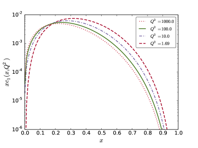
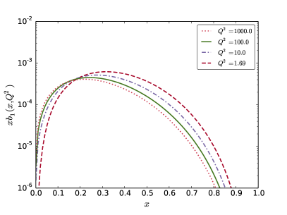
Figure 1: Scale-evolution of the IC (left) and IB (right) PDF at NLO according to the non-singlet evolution equation (11) using the Same Scales boundary condition in Eq. (17) with $m_{c}=1.3$ and $m_{b}=4.5$ GeV. Shown are results for $Q^{2}=1.69,10,100,1000$, and $10000$ GeV².

2.5 Numerical validation

In order to test the ideas presented in Secs. 2.2 and 2.3, we use the CTEQ6.6c series of intrinsic charm fits which have been obtained in the framework of the CTEQ6.6 global analysis Nadolsky:2008zw . The CTEQ6.6c series comprises 4 sets of PDFs including an intrinsic charm component. Two of them, CTEQ6.6c0 and CTEQ6.6c1, employ the BHPS model with $1\%$ and $3.5\%$ IC probability, respectively. This corresponds to the values of 0.01 and 0.035 of the first moment of the charm PDF, $\int dx\,c(x)$, calculated at the input scale $Q_{0}=m_{c}=1.3\ {\rm GeV}$. For a review of these models see Ref. Pumplin:2007wg . In the rest of this article, we will follow the naming convention of the CTEQ6.6c fits in which a given fit is characterized by the value in percentage of the first moment of the charm distribution at the input scale, e.g. 1% for CTEQ6.6c0. For convenience, we list below the first and second moments (calculated at the input scale) for the sets referred to in the following.

	$\int_{0}^{1}dx\;c(x)$	$\int_{0}^{1}dx\;x\left[c(x)+\bar{c}(x)\right]\equiv<x>_{c+\bar{c}}$
CTEQ6.6	0	0
CTEQ6.6c0	0.01	0.0057
CTEQ6.6c1	0.035	0.0200

As can be seen the actual momentum carried by the charm in the CTEQ6.6c0 and CTEQ6.6c1 fits is equal to $\sim 0.6$% and 2% respectively.

In the following we compare our approximate IC PDFs supplemented with the central CTEQ6.6 fit, which has a radiatively generated charm distribution, with the CTEQ6.6c0 and CTEQ6.6c1 sets where IC has been obtained from global analysis without the approximations of Sec. 2.2.

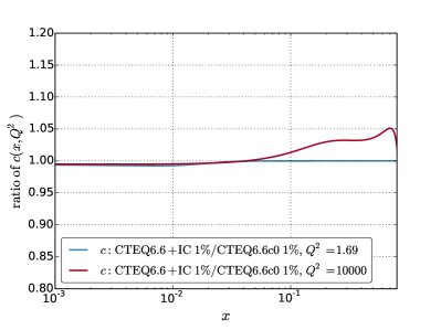
Figure 2: (a) CTEQ6.6c0 charm distribution function $c(x,Q^{2})$ (solid lines) and the sum $c_{0}(x,Q^{2})+c_{1}(x,Q^{2})$ (triangles) where $c_{0}$ is the radiatively generated CTEQ6.6 charm distribution and $c_{1}$ is the non-singlet evolved IC using the BHPS boundary condition (15) with the same normalization as used for the CTEQ6.6c0 charm distribution. Results are shown for the input scale $Q^{2}=Q_{0}^{2}=m_{c}^{2}$ and the scale $Q^{2}=10000\ {\rm GeV}^{2}$. Fig. (b) shows the ratio of the curves in (a).

In Fig. 2 the CTEQ6.6c0 charm distribution function $c(x,Q^{2})$ is shown (solid lines) for two scales, $Q^{2}=1.69$ and $10000\ {\rm GeV}^{2}$, in dependence of $x$. The doted lines have been obtained as the sum of $c_{0}(x,Q^{2})+c_{1}(x,Q^{2})$ where $c_{0}$ is the radiatively generated charm distribution using the CTEQ6.6 PDF and $c_{1}$ is the non-singlet evolved IC using the boundary condition (15) with the same normalization as used for the CTEQ6.6c0 charm distribution. As can be seen in the ratio plot, Fig. 2, the difference between the sum $c_{0}+c_{1}$ and the CTEQ6.6c0 charm distribution is tiny at low $Q^{2}$, and smaller than $5\%$ at the higher $Q^{2}$. In other words, the IC distribution $c_{1}$ evolved according to the decoupled non-singlet evolution equation is in very good agreement with the difference $c-c_{0}$ representing the IC component in the full global analysis.

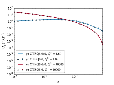
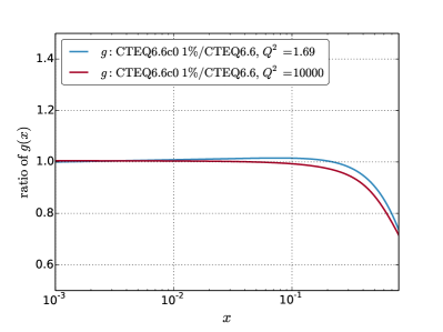
Figure 3: (a) Comparison of the CTEQ6.6c0 (solid line) and the CTEQ6.6 (triangles) gluon distributions. (b) Ratio of the CTEQ6.6c0 and the CTEQ6.6 gluon distributions. The results are shown as function of $x$ for two scales, $Q^{2}=1.69$ and $Q^{2}=10000\ {\rm GeV}^{2}$.

The inclusion of the intrinsic charm distribution will alter the other parton distributions, most notably the gluon PDF. In order to gauge this effect we compare in Fig. 3 the gluon distribution from the CTEQ6.6c0 analysis with the one from the standard CTEQ6.6 fit. Fig. 3 shows the $x$-dependence of the gluon distribution for two scales, $Q^{2}=1.69$ and $Q^{2}=10000\ {\rm GeV}^{2}$; Fig. 3 shows the ratio of these curves. For small $x$ ($x<0.1$) the gluon PDF is not affected by the presence of a BHPS-like intrinsic charm component which is concentrated at large $x$. At $x\simeq 0.7$, the CTEQ6.6c0 gluon is suppressed by about 20% with respect to CTEQ6.6, and this is relatively insensitive to the value of $Q^{2}$. We note that at large-$x$, the gluon distribution is already quite small and the uncertainty of the gluon PDF is sizable (of order of 40 – 50% for the CTEQ6.6 set). The difference between the gluon distributions is slightly enhanced when evolving from the input scale $Q^{2}=1.69\ {\rm GeV}^{2}$ to the electroweak scale $Q^{2}=10000\ {\rm GeV}^{2}$, but it is still much smaller than the PDF uncertainty. We conclude that for most applications, adding a standalone intrinsic charm distribution to an existing standard global analysis of PDFs is internally consistent and leads to only a small error. Moreover, for the case of intrinsic bottom which is additionally suppressed, the accuracy of the approximation will be even better.

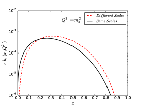
Figure 4: (a) Comparison of Different Scales, Eq. (16), and Same Scales, Eq. (17), boundary conditions for the IB PDF at the scale $Q=m_{b}=4.5\ {\rm GeV}$. Fig. (b) shows the ratio of the two curves in (a).

Another source of uncertainty is the choice of boundary conditions for the intrinsic distributions. For the IB PDF we have presented two equally compelling choices: the Different Scales ansatz of Eq. (16) and the Same Scales one of Eq. (17). In Fig. 4 we compare the Different Scales (dashed line) and the Same Scales boundary conditions (solid line) at the scale $Q=m_{b}=4.5\ {\rm GeV}$. As expected, the Same Scales boundary condition leads to a softer distribution due to the evolution from $m_{c}$ to $m_{b}$. The ratio of these two distributions varies between $2$ at small $x$ and $\frac{1}{2}$ at large $x$ (cf., Fig. 4). Note that the uncertainty due to the normalization is larger; for example, the ratio of the IC distributions $c_{1}(x,m_{b})$ from CTEQ6.6c1 and CTEQ6.6c0 is about 3.5. Furthermore, there is also a freedom in the parametric $m_{c}^{2}/m_{b}^{2}$ factor depending on which values are used for the heavy quark masses. Therefore, in the following we use the Same Scales boundary condition for our numerical studies and consider the normalization as a free parameter.

For completeness we also provide similar validation using the parton–parton luminosities

$$\frac{d\mathcal{L}_{ij}}{d\tau}(\tau,\mu)=\frac{1}{1+\delta_{ij}}\int_{\tau}^{1}\frac{dx}{x}\Big{[}f_{i}(x,\mu)f_{j}(\tau/x,\mu)+f_{j}(x,\mu)f_{i}(\tau/x,\mu)\Big{]},$$ (18)

where $\tau=x_{1}x_{2}$. We can consider the production of a heavy final state particle $H$ at the LHC ($pp\to H$) of mass $m_{H}^{2}=\hat{s}$, where $\hat{s}=x_{1}x_{2}S=\tau S$ so that $\tau=m_{H}^{2}/S$. This will allow us to estimate the effects of our approximation on the physical observables as a function of the mass scale $\sqrt{\tau}=m_{H}/\sqrt{S}$. We discuss the relation of the parton–parton luminosities to the actual cross-section in more detail in Sec. 3.2.

In Fig. 5 we show the ratio of $c\bar{c}$ luminosities for the IC with two choices of normalizations; we compare the results obtained with our approach to the CTEQ6.6c0 and CTEQ6.6c1 sets. We see that our error on the luminosities (the difference between corresponding solid and dashed lines) is smaller than 10% across the full range of $\tau=m_{H}^{2}/S$ values. Additionally, this error is much smaller than the difference between CTEQ6.6 and scenarios with IC (distance between blue band and red/green lines). Similarly, in Fig. 5 we show the ratio of luminosities for the $cg$ combination. In this case the error of our method is larger; it is around 10% for the IC 1% normalization, and it increases substantially for the case of IC 3.5% normalization. Note that for the IC 3.5% normalization, the deviation of our approximation from CTEQ6.6c1 is of the same order as the CTEQ6.6 PDF error band.

Thus, we conclude our approach provides a good approximation for $c\bar{c}$ luminosities for an IC with either 1% or 3.5% normalization. For $cg$ luminosities, this approximation is quite reasonable for an IC with 1% normalization; however, for 3.5% normalization, it is only sufficient to obtain a rough estimate of the effects. On the other hand, if the IC component is this large it should not be difficult to observe.

Since the IB case can be obtained by scaling IC with the $m_{c}^{2}/m_{b}^{2}$ suppression factor, our approximation will work perfectly well for both the $b\bar{b}$ and the $bg$ luminosities due to the smaller normalization.

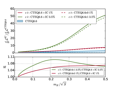
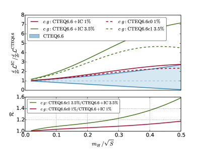
Figure 5: Parton–parton luminosities at the LHC with $\sqrt{S}=14$ TeV for (a) $\{c,\bar{c}\}$ and (b) $\{c,g\}$ calculated using: our IC and CTEQ6.6 PDFs (solid lines), CTEQ6.6c PDFs (dashed lines). For comparison, we show the PDF uncertainty (blue band) for the CTEQ6.6 PDFs. The upper plots show ratio of the corresponding luminosities compared to the result obtained with the central fit of CTEQ6.6. The lower plots present the ratio ${\cal R}$ of luminosities calculated using our IC plus CTEQ6.6 PDFs compared to the result with CTEQ6.6c0 (CTEQ6.6c1) PDFs. Note that the red curves represent cases with 1% IC normalization and the green ones cases with 3.5% IC normalization.

3 Possible effects of IC/IB on LHC observables

In this section, we investigate the effects of intrinsic heavy quarks on observables at the LHC. We study the effects of both IC and IB on parton–parton luminosities at 14 TeV LHC. This allows us to assess the relevance of a non-perturbative heavy quark component for the production of new heavy particles coupling to the SM fermions.

3.1 IB versus IC and prospects of observing IB

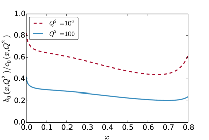
Figure 6: Ratio of the dynamically generated bottom and charm parton distributions at $Q^{2}=100$ and $Q^{2}=10^{6}$ GeV² as a function of $x$. The results for $x>0.7$ are not reliable due to instabilities in the CTEQ PDF grids for the charm distribution (note however, that for that large $x$ values the perturbative PDFs are nearly zero and are negligible).

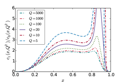
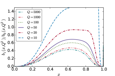
Figure 7: Ratio of intrinsic and dynamically generated heavy quark PDFs for (a) charm and (b) bottom quarks. The distributions $c_{1}(x,Q^{2})$ and $b_{1}(x,Q^{2})$ have been generated using the non-singlet evolution equation (11) with the BHPS form (15) (properly normalized to 1%) and the Same Scales boundary condition (17). $c_{0}(c,Q^{2})$ is the CTEQ6.6 charm distribution and $b_{0}(x,Q^{2})$ is the CTEQ6.6c0 bottom distribution. As in Fig. 6, the results in (a) are not reliable for $x>0.7$ due to instabilities in the CTEQ6.6 grids for very low values of the $c_{0}$ distribution.

The IB PDF is parametrically suppressed by a factor $m_{c}^{2}/m_{b}^{2}\simeq 1/10$ compared to the IC PDF. However, whenever particles have couplings to the SM fermions proportional to the fermion mass, the $m_{c}^{2}/m_{b}^{2}$ suppression will be compensated by a factor of $m_{b}^{2}$ in the coupling. In addition, the radiatively generated (extrinsic) bottom PDF is typically a factor of $\sim$1/5 to $\sim$1/2 smaller than the extrinsic charm PDF as shown in Fig. 6. Combining these pieces together we find $b_{1}/b_{0}<c_{1}/c_{0}$ which means that the possible effects due to the IB will be less pronounced than the ones due to the IC. The ratios $c_{1}/c_{0}$ and $b_{1}/b_{0}$ are shown for several scales in Figs. 7 and 7.

These figures are useful to illustrate the impact of the intrinsic heavy quark distributions on the physical observables. For this purpose, we define the ratio $\kappa_{c}=1+c_{1}/c_{0}$ and similarly $\kappa_{b}=1+b_{1}/b_{0}$ which measures the relative deviation expected due to the IC/IB components. For example, if the $b$-quark initiated subprocesses of an observable contributes a fraction $r_{b}$ to a cross section (say $r_{b}=80\%$), the observable will be enhanced by a factor $[r_{b}\times\kappa_{b}+(1-r_{b})]$ where $\kappa_{b}$ is evaluated at the $x$-value relevant for the specific process.

We note that $\kappa_{c}$ is still sizable at $Q=100\ {\rm GeV}$ with $\kappa_{c}\simeq 3$ ($\kappa_{c}\simeq 8$) for the case of 1% (3.5%) normalization. In contrast, the IB content is much smaller at this scale with $\kappa_{b}\simeq 1.6$ ($\kappa_{b}\simeq 3.1$) for the case of 1% (3.5%) normalization of the IC due to the $m_{c}^{2}/m_{b}^{2}$ factor. Therefore, we expect processes at the electroweak scale (or heavier scales) to be much less affected by the presence of an intrinsic bottom component. Nevertheless, in cases where a process is dominated by the $b$-quark initiated subprocesses and where the large $x$ region is probed (for example at large rapidities) an enhancement by a factor 1.6 (or even 3.1) might be visible. In general, processes probing lower scales ($Q<20\ {\rm GeV}$) and large $x$ ($x\gtrsim 0.5$) will be better suited to find/constrain the intrinsic bottom component of the nucleon.

3.2 Parton–parton luminosities at the LHC

We now turn our attention to the parton–parton luminosities and study the impact of a non-perturbative heavy quark component on these quantities for the LHC at 14 TeV. Using the factorization theorem of QCD for hadronic cross sections, one can express the inclusive cross section for the production of a heavy particle $H$ as follows:

$$\sigma_{pp\rightarrow H+X}=\sum_{ij}\int_{\tau}^{1}\int_{\tau/x_{1}}^{1}dx_{1}dx_{2}f_{i}(x_{1},\mu)f_{j}(x_{2},\mu)\hat{\sigma}_{ij\rightarrow H}(\hat{s})\ ,$$ (19)

where $\tau=x_{1}x_{2}=m_{H}^{2}/S$, $S$ is the hadronic center of mass energy, and $\hat{s}=x_{1}x_{2}S$ is its partonic counterpart. $f_{i}(x,\mu)$ denotes the PDF of parton $i$ carrying momentum fraction $x$ inside the proton. Finally, $\mu$ is the factorization scale which in the following is identified with the partonic center of mass energy $\hat{s}=m_{H}^{2}$. Equation (19) can be re-written in the form of a convolution of partonic cross-sections and parton–parton luminosities Quigg:2009gg ; Han:2014nja ,

$$\sigma_{pp\rightarrow H+X}=\sum_{ij}\int_{\tau}^{1}d\tau\ \displaystyle\frac{\mathcal{L}_{ij}}{d\tau}\ \hat{\sigma}_{ij}(\hat{s}),$$ (20)

where $\frac{d\mathcal{L}_{ij}}{d\tau}(\tau,\mu)$ has been introduced in Eq. (18). All the results of this section have been obtained using the CTEQ6.6 PDF set Nadolsky:2008zw supplemented with our approximate IC and IB PDFs constructed using the procedure presented in Sec. 2.

In Fig. 8 we show different parton–parton luminosities, $d\mathcal{L}_{ij}/d\tau$, for the LHC at 14 TeV (LHC14) as a function of $\sqrt{\tau}=m_{H}/\sqrt{S}$. We choose the range of $\sqrt{\tau}$ to be $[0.02,0.5]$ that corresponds to the production of a heavy particle of mass $m_{H}\in[0.280,7]$ TeV which is roughly the range of values that will likely be probed at the LHC14. As can be seen, at large $\sqrt{\tau}$, the parton–parton luminosities respect the following ordering: $ug\gg u\bar{u}>gg\gg gc>gb\gg c\bar{c}>b\bar{b}$. Consequently, one can generally conclude that heavy quark initiated subprocesses play a minor role in most processes where a heavy state is produced.

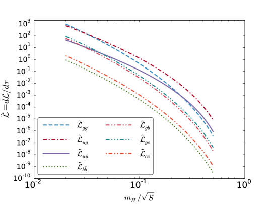
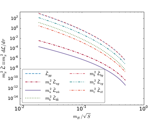
Figure 8: (a) Different parton–parton luminosities as a function of $\sqrt{\tau}=m_{H}/\sqrt{S}$ for the LHC14 calculated using CTEQ6.6 PDFs. For large $\tau$, the ordering of the curves is: $ug\gg u\bar{u}>gg\gg gc>gb\gg c\bar{c}>b\bar{b}$. (b) Rescaled parton–parton luminosities ($m_{i}^{2}d\mathcal{L}_{ij}/d\tau$) for the LHC14 calculated using CTEQ6.6 PDFs. For comparison, we also show the un-rescaled gluon–gluon luminosity. For large $\tau$, the ordering of the curves is: $gg\simeq gb>gc\gg b\bar{b}>c\bar{c}\gg ug\gg u\bar{u}$. Note that by coincidence the gluon–gluon luminosity, $\mathcal{L}_{gg}$, agrees at the 10% level with the scaled $gb$ luminosity, $m_{b}^{2}\mathcal{L}_{gb}$, so that the two curves lie on top of each other in (b).

One exception would be SM extensions where the couplings to the first two generations are suppressed or vanish so that the $gb$ or $b\bar{b}$ channels can dominate; typically this is done in order to avoid experimental constraints from low energy precision observables or flavor changing neutral currents. Of course, unless the couplings to the $gb$ or $b\bar{b}$ channels are enhanced, these scenarios have tiny cross sections and will be difficult to measure at the LHC.

However, if the couplings are enhanced by factors of the quark mass, the hierarchy of the contributions can change dramatically. This can happen when the heavy state has couplings to the Standard Model particles proportional to their masses such as the SM Higgs or the Higgs particles in 2HDM models. For example, in Fig. 8 we show the parton-parton luminosities with no enhancement factors; in Fig. 8 we show the same but with additional factors proportional to the heavy quark mass; the change is dramatic. Taking the quark masses into account, the high $\tau$ region now exhibits the following hierarchy: $gg\simeq gb>gc\gg b\bar{b}>c\bar{c}\gg ug\gg u\bar{u}$. In this case the heavy quark initiated subprocesses could play the dominant role, apart from the $gg$ initiated subprocesses which would contribute via an effective, model-dependent, heavy quark loop-induced $ggH$ coupling.

To explore how the presence of IC and IB would affect physics observables with a non-negligible heavy quark initiated subprocesses, in Fig. 9, we present the parton–parton luminosities $d\mathcal{L}/d\tau$, $d\mathcal{L}/d\tau$ with and without the intrinsic components. While the impact of the IC component for $\sqrt{\tau}>0.1$ is clearly visible, the corresponding effect for the bottom-quark is smaller and lies inside the PDF uncertainty band. Generally, the enhancement is larger for the processes initiated by two heavy quarks $\{c\bar{c},b\bar{b}\}$ since the intrinsic component is then “squared” in the luminosities.

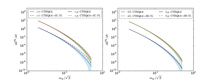
Figure 9: Parton–parton luminosities $d\mathcal{L}_{cg}/d\tau$, $d\mathcal{L}_{c\bar{c}}/d\tau$ (left) and $d\mathcal{L}_{bg}/d\tau$, $d\mathcal{L}_{b\bar{b}}/d\tau$ (right) at the LHC14 as a function of $\sqrt{\tau}=m_{H}/\sqrt{S}$. Shown are results without an intrinsic heavy quark component using the CTEQ6.6 PDFs (solid lines) including the band due to the PDF uncertainties and the same quantities calculated with addition of IC normalized to 1% and the corresponding IB component (dashed lines).

In order to precisely quantify the impact of the intrinsic components in Figs. 10 and 11 we show the ratios of luminosities for charm and bottom with and without an intrinsic contribution for 1% and 3.5% normalizations. Furthermore, since there are no experimental constraints on the IB normalization, in Fig. 11 we also include an extreme scenario where we remove the usual $m_{c}^{2}/m_{b}^{2}$ factor; thus, the first moment of the IB is 1% at the initial scale $m_{c}$.

For the 1% normalization the $c\bar{c}$ luminosity ratio grows as large as 7 or 8 for $\sqrt{\tau}=0.5$, and for a 3.5% normalization it becomes extremely large and reaches values of up to 50. From these figures we can clearly see that the effect of the 3.5% IC is substantial and can affect observables sensitive to $c\bar{c}$ and $cg$ channels. As expected, in the case of IB the effect is smaller but for the $b\bar{b}$ luminosity the IB with 3.5% normalization leads to a curve which lies clearly above the error band of the purely perturbative result. In the extreme scenario (which is not likely but by no means excluded) the IB component has a big effect on both the $b\bar{b}$ and $bg$ channels.

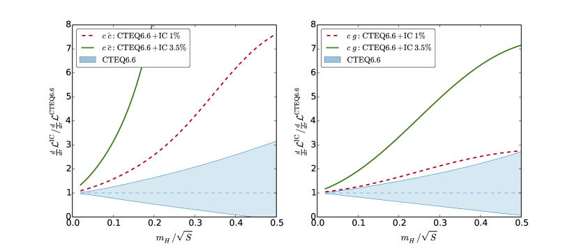
Figure 10: Ratio of $c\bar{c}$ luminosities (left) and $cg$ luminosities (right) at the LHC14 for charm-quark PDF sets with and without an intrinsic component as a function of $\sqrt{\tau}=m_{H}/\sqrt{S}$. The ratio for the $c\bar{c}$ luminosity (solid, green line) in the left figure reaches values of 50 at $\sqrt{\tau}=0.5$. In addition to the curves with 1% normalization (red, dashed lines) we include the results for the 3.5% normalization (green, solid lines) which was found to be still compatible with the current data Nadolsky:2008zw .

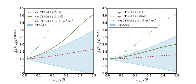
Figure 11: Ratio of luminosities at the LHC14 for bottom-quark PDF sets with different normalizations of the intrinsic bottom component. The plot has been truncated, and the $b\bar{b}$ luminosity in the extreme scenario reaches about 17 at $\sqrt{\tau}=0.5$.

4 Discussion

We have demonstrated that the scale evolution of intrinsic heavy quark distributions (both charm and bottom) is governed by a non-singlet evolution equation to a very good approximation. Furthermore, the small intrinsic heavy quark distribution does not significantly influence the other parton distributions or the sum rules of a global analysis. This observation holds to a very good precision for the intrinsic bottom case, but also works reasonably well for the intrinsic charm case (if the momentum fraction is not too large). Therefore, it is possible to perform a standalone analysis of the intrinsic heavy quark distribution and to combine it with the PDFs of a standard global analysis with dynamically generated heavy quark distributions. Note, this allows us to use any general PDF set and generate a matched IC or IB component without a global fit re-analysis.

Based on this observation we have modeled an intrinsic bottom distribution and discussed its effect on the relevant parton–parton luminosities at the LHC14. As a general rule, the effects of IB are less pronounced than the ones from IC due to the expected $m_{c}^{2}/m_{b}^{2}\sim 0.1$ suppression factor. For example, we see from Fig. 7 (1% normalization) that whereas $\kappa_{c}=1+c_{1}/c_{0}\sim 3$ at scales $Q\sim 100$ GeV and $x\in[0.4,0.8]$ the corresponding factor for IB is relatively small: $\kappa_{b}=1+b_{1}/b_{0}\lesssim 1.4$. For a 3.5% normalization, the curves in Fig. 7 would be scaled by a factor 3.5, such that $\kappa_{b}\lesssim 2.4$.

We then turned to a discussion of the parton–parton luminosities where the main results can be seen in Figs. 10 and 11.

The $c\bar{c}$ luminosities are strongly enhanced for the IC with both 1% and 3.5% normalization as the heavy quark factors enter quadratically; but the effect is smaller for the $cg$ luminosity as there is only one factor of the heavy quark PDF. However, the effect is still significant; the 1% IC lies at the edge of the PDF uncertainty band, and the 3.5% IC yields a factor of $\sim$5.

As expected, the enhancement of the $b\bar{b}$ luminosity is much smaller compared to the $c\bar{c}$ case. For the 1% IB the curve lies well within the PDF uncertainty band. For the 3.5% IB the results lies above this uncertainty band and predicts an enhancement of a factor 4 at $\sqrt{\tau}=0.5$. For the $bg$ luminosity, both the 1% IB and the 3.5% IB curves lie within the PDF uncertainty band. This band is largely driven by the uncertainty of the gluon distribution and might shrink in the future such that the enhancement due to the IB could become significant. For illustration, we have also included results for the extreme assumption that the probability (first moment) for IB is 1%. In this case the enhancement is sizable and reaches a factor 17 for the $b\bar{b}$ case and a factor 4 for the $bg$ case at $\sqrt{\tau}=0.5$.

In view of this, we can address the impact of IB on heavy new physics and certain electroweak processes where the $bg$ or the $b\bar{b}$ channel plays an important role. For the 1% and 3.5% IB the enhancement for the $bg$-initiated subprocesses would be hidden within the PDF uncertainties. The $b\bar{b}$-initiated subprocesses could be significantly enhanced in the case of 3.5% IB. The effect would be more pronounced for heavier states where however, the $b\bar{b}$ luminosity is extremely small so that a measurement would be limited by statistics even for models with enhanced couplings to the $b$ quark. All in all, we conclude that the IB will have limited impact on searches for heavy new physics at the LHC.

5 Conclusions

In this article, we presented a method to generate a matched IC/IB distributions for any PDF set without the need for a complete global re-analysis. This allows one to easily carry out a consistent analysis including intrinsic heavy quark effects. Because the evolution equation for the intrinsic heavy quarks decouples, we can freely adjust the normalization of the IC/IB PDFs.

For the IB, our approximation holds to a very good precision. For the IC, the error increases (because the IC increases), yet our method is still useful. For an IC normalization of 1-2%, the error is less than the PDF uncertainties at the large-$x$ where the IC is relevant. For a larger normalization, although the error may be the same order as the PDF uncertainties, the IC effects also grow and can be separately distinguished from the case without IC. In any case, the IC/IB represents a non-perturbative systematic effect which should be taken into account.

The method presented here greatly simplifies our ability to search for, and place constraints upon, intrinsic charm and bottom compoments of the nucleon. This technique will facilitate more precise predictions which may be observed at future facilities such as an Electron Ion Collider (EIC), the Large Hadron-Electron collider (LHeC), or AFTER and LHC.

The PDF sets for intrinsic charm and intrinsic bottom discussed in this analysis (1% IC, 3.5% IC, 1% IB, 3.5% IB) are available from the authors upon request.

References

- (1) F. Maltoni, G. Ridolfi, and M. Ubiali, -initiated processes at the LHC: a reappraisal, JHEP 1207 (2012) 022, [1203.6393].
- (2) G. Altarelli and G. Parisi, Asymptotic Freedom in Parton Language, Nucl. Phys. B126 (1977) 298.
- (3) V. N. Gribov and L. N. Lipatov, Deep inelastic scattering in perturbation theory, Sov. J. Nucl. Phys. 15 (1972) 438–450.
- (4) Y. L. Dokshitzer, Calculation of the Structure Functions for Deep Inelastic Scattering and Annihilation by Perturbation Theory in Quantum Chromodynamics (In Russian), Sov. Phys. JETP 46 (1977) 641–653.
- (5) J. C. Collins and W.-K. Tung, Calculating Heavy Quark Distributions, Nucl. Phys. B278 (1986) 934.
- (6) M. Buza, Y. Matiounine, J. Smith, and W. L. van Neerven, Charm electroproduction viewed in the variable-flavour number scheme versus fixed-order perturbation theory, Eur. Phys. J. C1 (1998) 301–320, [hep-ph/9612398].
- (7) M. Aivazis, J. C. Collins, F. I. Olness, and W.-K. Tung, Leptoproduction of heavy quarks. 2. A Unified QCD formulation of charged and neutral current processes from fixed target to collider energies, Phys.Rev. D50 (1994) 3102–3118, [hep-ph/9312319].
- (8) J. C. Collins, Hard scattering factorization with heavy quarks: A General treatment, Phys.Rev. D58 (1998) 094002, [hep-ph/9806259].
- (9) S. Forte, E. Laenen, P. Nason, and J. Rojo, Heavy quarks in deep-inelastic scattering, Nucl.Phys. B834 (2010) 116–162, [1001.2312].
- (10) M. Cacciari, M. Greco, and P. Nason, The P(T) spectrum in heavy flavor hadroproduction, JHEP 9805 (1998) 007, [hep-ph/9803400].
- (11) R. Thorne, Heavy quarks in DIS (theory), J.Phys. G25 (1999) 1307–1312, [hep-ph/9902299].
- (12) A. Belyaev, J. Pumplin, W.-K. Tung, and C. P. Yuan, Uncertainties of the inclusive Higgs production cross section at the Tevatron and the LHC, JHEP 01 (2006) 069, [hep-ph/0508222].
- (13) S. J. Brodsky, P. Hoyer, C. Peterson, and N. Sakai, The Intrinsic Charm of the Proton, Phys. Lett. B93 (1980) 451–455.
- (14) S. J. Brodsky, C. Peterson, and N. Sakai, Intrinsic Heavy Quark States, Phys.Rev. D23 (1981) 2745.
- (15) F. S. Navarra, M. Nielsen, C. A. A. Nunes, and M. Teixeira, On the intrinsic charm component of the nucleon, Phys. Rev. D54 (1996) 842–846, [hep-ph/9504388].
- (16) S. Paiva, M. Nielsen, F. S. Navarra, F. O. Duraes, and L. L. Barz, Virtual meson cloud of the nucleon and intrinsic strangeness and charm, Mod. Phys. Lett. A13 (1998) 2715–2724, [hep-ph/9610310].
- (17) W. Melnitchouk and A. W. Thomas, HERA anomaly and hard charm in the nucleon, Phys. Lett. B414 (1997) 134–139, [hep-ph/9707387].
- (18) J. Pumplin, Light-Cone Models for Intrinsic Charm and Bottom, Phys. Rev. D73 (2006) 114015, [hep-ph/0508184].
- (19) European Muon Collaboration Collaboration, J. Aubert et. al., Production of charmed particles in 250-GeV - iron interactions, Nucl.Phys. B213 (1983) 31.
- (20) European Muon Collaboration Collaboration, J. Aubert et. al., An Experimental Limit on the Intrinsic Charm Component of the Nucleon, Phys.Lett. B110 (1982) 73.
- (21) E. Hoffmann and R. Moore, Subleading contributions to the intrinsic charm of the nucleon, Z.Phys. C20 (1983) 71.
- (22) B. Harris, J. Smith, and R. Vogt, Reanalysis of the EMC charm production data with extrinsic and intrinsic charm at NLO, Nucl.Phys. B461 (1996) 181–196, [hep-ph/9508403].
- (23) F. M. Steffens, W. Melnitchouk, and A. W. Thomas, Charm in the nucleon, Eur. Phys. J. C11 (1999) 673–683, [hep-ph/9903441].
- (24) J. Pumplin, H. L. Lai, and W. K. Tung, The Charm Parton Content of the Nucleon, Phys. Rev. D75 (2007) 054029, [hep-ph/0701220].
- (25) P. M. Nadolsky et. al., Implications of CTEQ global analysis for collider observables, Phys. Rev. D78 (2008) 013004, [0802.0007].
- (26) A. Martin, W. Stirling, R. Thorne, and G. Watt, Parton distributions for the LHC, Eur.Phys.J. C63 (2009) 189–285, [0901.0002].
- (27) NNPDF Collaboration, R. D. Ball et. al., Parton distributions for the LHC Run II, 1410.8849.
- (28) S. Dulat, T.-J. Hou, J. Gao, J. Huston, J. Pumplin, et. al., Intrinsic Charm Parton Distribution Functions from CTEQ-TEA Global Analysis, Phys.Rev. D89 (2014), no. 7 073004, [1309.0025].
- (29) J. Gao, M. Guzzi, J. Huston, H.-L. Lai, Z. Li, et. al., CT10 next-to-next-to-leading order global analysis of QCD, Phys.Rev. D89 (2014), no. 3 033009, [1302.6246].
- (30) P. Jimenez-Delgado, T. Hobbs, J. Londergan, and W. Melnitchouk, New limits on intrinsic charm in the nucleon from global analysis of parton distributions, Phys.Rev.Lett. 114 (2015), no. 8 082002, [1408.1708].
- (31) S. Brodsky and S. Gardner, Comment on ”New Limits on Intrinsic Charm in the Nucleon from Global Analysis of Parton Distributions”, 1504.00969.
- (32) D. Boer, M. Diehl, R. Milner, R. Venugopalan, W. Vogelsang, et. al., Gluons and the quark sea at high energies: Distributions, polarization, tomography, 1108.1713. arXiv:1108.1713.
- (33) N. Y. Ivanov, The Ratio in DIS as a Probe of the Charm Content of the Proton, Nucl.Phys. B814 (2009) 142–155, [0812.0722].
- (34) L. Ananikyan and N. Y. Ivanov, Azimuthal Asymmetries in DIS as a Probe of Intrinsic Charm Content of the Proton, Nucl.Phys. B762 (2007) 256–283, [hep-ph/0701076].
- (35) L. Ananikyan and N. Y. Ivanov, Azimuthal dependence of the heavy quark initiated contributions to DIS, Phys.Rev. D75 (2007) 014010, [hep-ph/0609074].
- (36) B. A. Kniehl, G. Kramer, I. Schienbein, and H. Spiesberger, Inclusive production in collisions with massive charm quarks, Phys. Rev. D71 (2005) 014018, [hep-ph/0410289].
- (37) B. Kniehl, G. Kramer, I. Schienbein, and H. Spiesberger, Collinear subtractions in hadroproduction of heavy quarks, Eur.Phys.J. C41 (2005) 199–212, [hep-ph/0502194].
- (38) B. Kniehl, G. Kramer, I. Schienbein, and H. Spiesberger, Hadroproduction of and mesons in a massive VFNS, AIP Conf.Proc. 792 (2005) 867–870, [hep-ph/0507068].
- (39) H. Spiesberger, Inclusive D-Meson Production at the LHC, 1205.7000.
- (40) B. Kniehl, G. Kramer, I. Schienbein, and H. Spiesberger, Inclusive Charmed-Meson Production at the CERN LHC, Eur.Phys.J. C72 (2012) 2082, [1202.0439].
- (41) B. Kniehl, G. Kramer, I. Schienbein, and H. Spiesberger, Inclusive B-Meson Production at the LHC in the GM-VFN Scheme, Phys.Rev. D84 (2011) 094026, [1109.2472].
- (42) B. A. Kniehl, G. Kramer, I. Schienbein, and H. Spiesberger, Open charm hadroproduction and the charm content of the proton, Phys. Rev. D79 (2009) 094009, [0901.4130].
- (43) LHCb collaboration Collaboration, R. Aaij et. al., Prompt charm production in pp collisions at sqrt(s)=7 TeV, Nucl.Phys. B871 (2013) 1–20, [1302.2864].
- (44) K. Kovarik and T. Stavreva, Constraining the Intrinsic Heavy Quark PDF via Direct Photon Production in Association with a Heavy Quark Jet, 1206.2175.
- (45) D0 Collaboration, V. M. Abazov et. al., Measurement of + b + X and + c + X production cross sections in collisions at =1.96 TeV, Phys. Rev. Lett. 102 (2009) 192002, [0901.0739].
- (46) D0 Collaboration Collaboration, V. M. Abazov et. al., Measurement of the photon-jet production differential cross section in collisions at TeV, Phys.Lett. B714 (2012) 32–39, [1203.5865].
- (47) T. P. Stavreva and J. F. Owens, Direct Photon Production in Association With A Heavy Quark At Hadron Colliders, Phys. Rev. D79 (2009) 054017, [0901.3791].
- (48) T. Stavreva, I. Schienbein, F. Arleo, K. Kovarik, F. Olness, et. al., Probing gluon and heavy-quark nuclear PDFs with production in collisions, JHEP 1101 (2011) 152, [1012.1178].
- (49) T. Stavreva, F. Arleo, and I. Schienbein, Probing nuclear parton densities and parton energy loss processes through photon + heavy-quark jet production in p-A and A-A collisions, J.Phys.G G38 (2011) 124187, [1109.2050].
- (50) V. Bednyakov, M. Demichev, G. Lykasov, T. Stavreva, and M. Stockton, Searching for intrinsic charm in the proton at the LHC, Phys.Lett. B728 (2014) 602–606.
- (51) V. Bednyakov, M. Demichev, G. Lykasov, T. Stavreva, and M. Stockton, Searching for intrinsic charm in the proton at the LHC, EPJ Web Conf. 60 (2013) 20047, [1305.3548].
- (52) S. Brodsky, F. Fleuret, C. Hadjidakis, and J. Lansberg, Physics Opportunities of a Fixed-Target Experiment using the LHC Beams, Phys.Rept. 522 (2013) 239–255, [1202.6585].
- (53) J. Lansberg, S. Brodsky, F. Fleuret, and C. Hadjidakis, Quarkonium Physics at a Fixed-Target Experiment using the LHC Beams, Few Body Syst. 53 (2012) 11–25, [1204.5793].
- (54) J. Lansberg, R. Arnaldi, S. Brodsky, V. Chambert, J. Didelez, et. al., AFTER@LHC: a precision machine to study the interface between particle and nuclear physics, EPJ Web Conf. 66 (2014) 11023, [1308.5806].
- (55) A. Rakotozafindrabe, M. Anselmino, R. Arnaldi, E. Scomparin, S. Brodsky, et. al., Studying the high x frontier with A Fixed-Target ExpeRiment at the LHC, PoS DIS2013 (2013) 250, [1310.6195].
- (56) Brodsky, S. J. et al., “A review of the intrinsic heavy quark content of the nucleon.” Preprint: MITP/15-027, LPSC-15-082, SLAC-PUB-16258.
- (57) A. Vogt, S. Moch, and J. A. M. Vermaseren, The three-loop splitting functions in QCD: The singlet case, Nucl. Phys. B691 (2004) 129–181, [hep-ph/0404111].
- (58) S. Moch, J. A. M. Vermaseren, and A. Vogt, The three-loop splitting functions in QCD: The non-singlet case, Nucl. Phys. B688 (2004) 101–134, [hep-ph/0403192].
- (59) A. Vogt, Efficient evolution of unpolarized and polarized parton distributions with QCD-PEGASUS, Comput.Phys.Commun. 170 (2005) 65–92, [hep-ph/0408244].
- (60) C. Quigg, LHC Physics Potential versus Energy, 0908.3660.
- (61) T. Han, J. Sayre, and S. Westhoff, Top-Quark Initiated Processes at High-Energy Hadron Colliders, 1411.2588.