Confinement-deconfinement transition due to spontaneous symmetry breaking in quantum Hall bilayers

Abstract

Band-inverted electron-hole bilayers support quantum spin Hall insulator and exciton condensate phases. We investigate such a bilayer in an external magnetic field. We show that the interlayer correlations lead to formation of a helical quantum Hall exciton condensate state. In contrast to the chiral edge states of the quantum Hall exciton condensate in electron-electron bilayers, existence of the counterpropagating edge modes results in formation of a ground state spin-texture not supporting gapless single-particle excitations. This feature has deep consequences for the low energy behavior of the system. Namely, the charged edge excitations in a sufficiently narrow Hall bar are confined i.e. a charge on one of the edges always gives rise to an opposite charge on the other edge. Moreover, we show that magnetic field and gate voltages allow to control confinement-deconfinement transition of charged edge excitations, which can be probed with nonlocal conductance. Confinement-deconfinement transitions are of great interest, not least because of their possible significance in shedding light on the confinement problem of quarks.

The role of the electron-electron interactions for the experimentally accessible topological media is best appreciated in quantum Hall (QH) systems. The fractionally charged quasiparticles have been studied at the fractional filling factors Sarma and Pinczuk (2008); Jain (2007), and the non-abelian excitations of more exotic QH states may eventually lead to a revolution in quantum computing Read and Green (2000); Nayak et al. (2008); Lindner et al. (2012); Clarke et al. (2013); Mong et al. (2014). However, Coulomb interactions play a crucial role also in the case of the integer filling factors Chakraborty and Pietiläinen (1987); Fertig (1989); Sondhi et al. (1993); Moon et al. (1995); Sarma and Pinczuk (2008); Eisenstein and MacDonald (2004); Girvin (1999). Remarkably, interactions create a QH ferromagnetic ground state at $\nu=1$ even in the absence of Zeeman energy. In such systems, the $SU(2)$ spin rotation symmetry is spontaneously broken, resulting in the low-energy excitations being spin waves and charged topological spin textures, skyrmions Moon et al. (1995); Sarma and Pinczuk (2008); Girvin (1999); Sondhi et al. (1993). The presence of a small symmetry-breaking Zeeman field does not change the low-energy excitations qualitatively.

In QH bilayer systems the role of spin is played by the layer index (pseudospin) Chakraborty and Pietiläinen (1987); Fertig (1989); Moon et al. (1995); Girvin (1999). In this case the $SU(2)$ pseudospin rotation symmetry is explicitly broken by the interactions, as they are larger within the layers than between the layers. The interactions favor the pseudospin orientations in $(x,y)$-plane, where the direction is chosen spontaneously (spontaneous $U(1)$ symmetry breaking) so that the QH bilayers realize an easy-plane ferromagnet. Since the spontaneously chosen direction in the $(x,y)$-plane corresponds to a spontaneous interlayer phase coherence, this easy-plane ferromagnetic state is equivalent to an exciton condensate Fertig (1989); Moon et al. (1995).

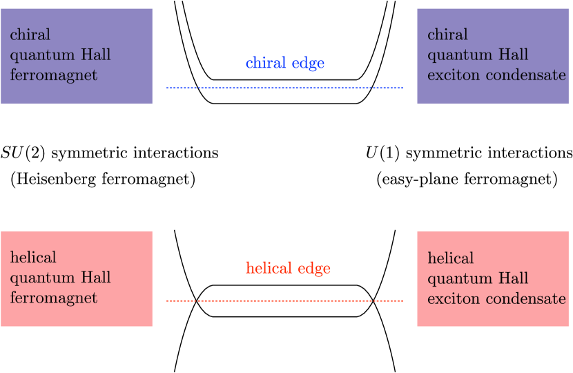
Figure 1: Four different types of experimentally accessible QH pseudospin ferromagnetic states at $\nu=1$. The single layer realizations (left column) realize Heisenberg ferromagnets because the interactions have $SU(2)$ symmetry. The bilayer QH exciton condensates (right column) can be described as an easy-plane ferromagnet with a spontaneously broken $U(1)$-symmetry. We argue that the classification is additionally enriched as the QH systems can support either chiral (top row) or helical (bottom row) edge excitations.

The QH ferromagnet and QH exciton condensate in electron-electron bilayers support a single chiral edge mode. However the two Landau levels may also support counterpropagating edge modes. The natural hosts of such kind of QH states are systems supporting quantum spin Hall (QSH) effect Kane and Mele (2005); Bernevig et al. (2006); König et al. (2007); Liu et al. (2008); Du et al. (2013); Spanton et al. (2014) due to inverted electron-hole bandstructure. In these materials the magnetic field allows to tune through the Landau level crossing Scharf et al. (2012); Pikulin et al. (2014), where we expect to find a QH state with spontaneously-broken (pseudo)spin-rotation symmetry. Thus, we argue that there exist four different experimentally accessible pseudospin ferromagnetic states, determined by spontaneously broken symmetry [SU(2) in single layer and U(1) in bilayer systems] and the edge structure [chiral or helical]. All these possibilities are illustrated in Fig. 1.

In this paper we concentrate on the helical QH exciton condensate state [broken U(1) symmetry and helical edge structure]. Remarkably, we find that in this system the charged edge excitations in a sufficiently narrow Hall bar are confined: A charge on one of the edges is always connected to the opposite charge on the other edge through the bulk by a stripe of rotated pseudospins, and thus low-energy isolated charged excitations cannot be observed. The gapless single-particle excitations are prohibited since the electron-electron interactions lead to an edge reconstruction and opening of a single-particle gap Iordanskii99 ; Fertig06 . However, unlike it happens in the existing examples, the helical exciton condensate creates long-range correlations between edges. We show that a magnetic field and gate voltages can be used to tune in and out of the exciton condensate phase. Thus this system provides a unique opportunity to study a confinement-deconfinement transition, similar to the one which is hypothesized to liberate the quarks from their color confinement at extremely high temperatures or densities Greensite (2011). Finally, we show that the confined and deconfined phases can be distinguished using nonlocal conductance.

I Helical quantum Hall exciton condensate phase

We consider bilayer QSH systems, such as InAs/GaSb Liu et al. (2008); Du et al. (2013); Spanton et al. (2014), described by the BHZ Hamiltonian Bernevig et al. (2006); Liu et al. (2008); supplementary . The important property of these systems is that there is a crossing of electron and hole Landau levels as a function of magnetic field at $B=B_{\rm cross}$ Scharf et al. (2012); Pikulin et al. (2014); supplementary [see Fig. 2(a)], where the band inversion is removed. Near this crossing the single-particle Hamiltonian is supplementary

$$\hat{H}_{0}=\sum_{k}[\hat{\psi}_{k,\uparrow}^{\dagger}\hat{\psi}_{k,\uparrow}-\hat{\psi}_{k,\downarrow}^{\dagger}\hat{\psi}_{k,\downarrow}]E_{G}(kl_{B}^{2}),$$ (1)

where $E_{G}(y)=E_{G}(kl_{B}^{2})$ is the energy-momentum dispersion of Landau levels and $\hat{\psi}^{\dagger}_{k\uparrow(\downarrow)}$ are the electron creation operators for the lowest electron and hole Landau levels. Here we have fixed the total filling factor of the Landau levels $\nu_{T}=\nu_{\uparrow}+\nu_{\downarrow}=1$, and utilized the fact that the momentum $k$ in the Landau level wavefunctions is directly connected to the position $y$ in the real space. Importantly, the spin and layer degrees of freedom are locked with each other, so that the pseudospin $\uparrow(\downarrow)$ means simultaneously up (down) spin and upper (lower) layer supplementary . The Fermi level is set to be at zero energy.

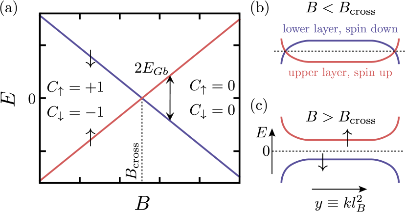
Figure 2: Magnetic field and momentum dependence of the lowest Landau level energies. (a) There exists a robust crossing of the lowest Landau level energies as a function of magnetic field at $B=B_{\rm cross}$, because the energy of the electron-like Landau level with spin up (red line) increases and the energy of the hole Landau level with spin down (blue line) decreases as a function of $B$. We denote the energy separation between these two levels as $2E_{Gb}$. (b-c) Momentum (or equivalently position) dependencies of the lowest Landau level energies. The electron-like (hole-like) Landau level bends upwards (downwards) in energy near the edge of the sample. (b) For $B<B_{\rm cross}$ the system supports helical edge modes protected by spin-resolved Chern numbers $C_{\uparrow}=-C_{\downarrow}=1$. (c) For $B>B_{\rm cross}$ the edge is gapped according to the non-interacting theory ($C_{\uparrow}=C_{\downarrow}=0$).

In the bulk the energy $E_{G}(y)=E_{Gb}$ is independent of the momentum ($E_{Gb}<0$ for $B<B_{\rm cross}$ and $E_{Gb}>0$ for $B>B_{\rm cross}$). When approaching the edge the Landau level originating from the electron (hole) band always disperses upwards (downwards) in energy. The spatial variation of $E_{G}(y)$ occurs within a characteristic length scale $l_{0}\gtrsim l_{B}$, which depends on the details of the edge, but due to topological reasons $E_{G}(y)>0$ reaches extremely large values (on the order of the energy separation between the bulk Landau levels) close to the edge supplementary . Therefore, for the magnetic fields $B<B_{\rm cross}$, $E_{G}(y)$ goes through zero near the edge, yielding to the helical edge states [see Fig. 2(b)]. On the other hand for $B>B_{\rm cross}$ the edge is gapped in the non-interacting theory [see Fig. 2(c)].

The electron-electron interactions $\hat{H}_{I}$ are described by

$$\hat{H}_{I}=\frac{1}{2}\sum_{\sigma,\sigma^{\prime}}\sum_{k,k^{\prime},q}V_{P}^{\sigma\sigma^{\prime}}(k-k^{\prime},q)\hat{\psi}_{k\sigma}^{\dagger}\hat{\psi}_{k^{\prime},\sigma^{\prime}}^{\dagger}\hat{\psi}_{k^{\prime}+q\sigma^{\prime}}\hat{\psi}_{k-q\sigma},$$ (2)

where $V_{P}^{\sigma\sigma^{\prime}}(k-k^{\prime},q)$ is obtained by projecting the Coulomb interactions to the subspace generated by the wavefunctions of the lowest Landau levels supplementary . Here, we assumed that the higher Landau levels are energetically separated from the lowest ones by an energy gap larger than the characteristic energy scale of the Coulomb interactions $V_{C}=e^{2}/(4\pi\epsilon\epsilon_{0}l_{B})$. We find that this assumption can be satisfied with the material parameters corresponding to InAs/GaSb bilayers Liu and Zhang (2013).

To find the ground state of the Hamiltonian $\hat{H}=\hat{H}_{0}+\hat{H}_{I}$, we consider states where the local direction of the pseudospin $\mathbf{h}(\mathbf{r})$ ($|\mathbf{h}(\mathbf{r})|=1$) varies in space. Because the Hamiltonian is translationally invariant in the $x$-direction, we assume that $\mathbf{h}(\mathbf{r})$ is independent of $x$ comment . By further noticing that the $y$-dependence translates to a momentum dependence of the pseudospin $h_{i}(y)=h_{i}(kl_{B}^{2})$, we can express our ansatz for the ground state many-particle wavefunction as a Slater determinant $|\Psi[\mathbf{h}(kl_{B}^{2})]\rangle$, where for each momentum $k$ we create an electron with pseudospin pointing along $\mathbf{h}(kl_{B}^{2})$. To compute the ground state, we need to minimize the energy functional for such kind of pseudospin texture Moon et al. (1995). For the energy functional we obtain supplementary

$$E = E_{0}-\sum_{k,k^{\prime}}\bigg{\{}\sum_{i=x,y}V_{P}^{XY}(k-k^{\prime})h_{i}(kl_{B}^{2})h_{i}(k^{\prime}l_{B}^{2})$$

$$+V_{P}^{Z}(k-k^{\prime})h_{z}(kl_{B}^{2})h_{z}(k^{\prime}l_{B}^{2})\bigg{\}}+\sum_{k}E_{G}(kl_{B}^{2})h_{z}(kl_{B}^{2}).$$

Here $V^{Z}_{P}(q)=[-V_{P}^{\uparrow\uparrow}(q,0)+V_{P}^{\uparrow\uparrow}(q,q)+V_{P}^{\uparrow\downarrow}(q,0)]/4$ and $V_{P}^{XY}(q)=V_{P}^{\uparrow\downarrow}(q,q)/4$ are the interaction coefficients, which characterize the anisotropy of the interactions within a layer and between the layers.

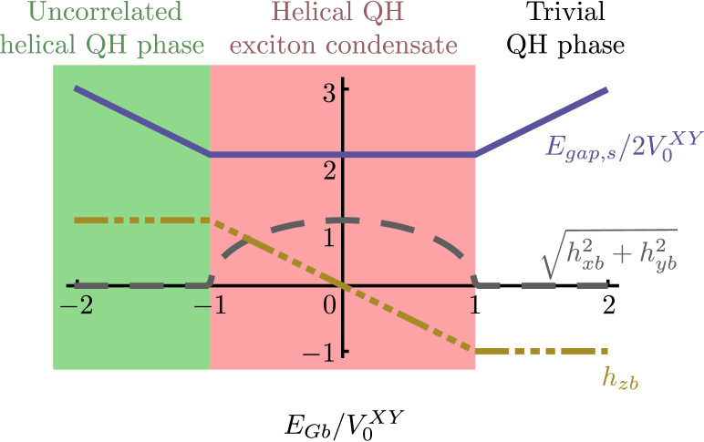
Figure 3: Phase diagram. For $E_{Gb}<-2(V^{XY}_{0}-V^{Z}_{0})$ the system supports an uncorrelated helical QH phase. In this phase, there is no spontaneous interlayer phase coherence in the bulk ($h_{xb}^{2}+h_{yb}^{2}=0$) and the system supports helical edge states (guaranteed by spin-resolved Chern numbers $C_{\uparrow/\downarrow}=\pm 1$). For $|E_{Gb}|<2(V^{XY}_{0}-V^{Z}_{0})$ the system supports a helical QH exciton condensate phase. In this phase, there is spontaneous interlayer phase coherence ($h_{xb}^{2}+h_{yb}^{2}\neq 0$), and the system supports exotic confined edge excitations (see below). For $E_{Gb}>2(V^{XY}_{0}-V^{Z}_{0})$ the system is in a trivial QH phase, where the edge is fully gapped. $E_{Gb}$ can be controlled with gate voltages or magnetic field comment2 . Charged bulk excitations are gapped everywhere in the phase diagram ($E_{\rm gap,s}>0$). We have chosen $V_{0}^{Z}/V_{0}^{XY}=1/2$.

We start by considering an infinite system. In this case, the pseudospin direction $\mathbf{h}(\mathbf{r})$ is spatially homogeneous. By minimizing the energy-functional (LABEL:energyfunctional), we find that the pseudospin direction $\mathbf{h}_{b}$ is determined by the parameters $E_{Gb}$ and $V^{Z(XY)}_{0}=\sum_{q}V^{Z(XY)}_{P}(q)$ supplementary . Here $E_{Gb}$ acts as an effective magnetic field preferring the pseudospin direction along $-{\rm sgn}(E_{Gb})\hat{e}_{z}$. On the other hand, the interactions prefer the pseudospin directions within the (x,y)-plane ($V^{XY}_{0}>V^{Z}_{0}$), and the energy cost to rotate the pseudospin so that it points along the $z$-direction is proportional to $V^{XY}_{0}-V^{Z}_{0}$. Thus, as a balance between these two competing effects, the direction of the pseudospin is tilted away from the $(x,y)$-plane, resulting in the three distinct phases of the system, which are summarized in Fig. 3. For sufficiently large $|E_{Gb}|$, we see that $|h_{zb}|=1$, meaning that only one layer is occupied. The phases $h_{zb}=1$ (uncorrelated helical QH phase) and $h_{zb}=-1$ (trivial QH phase) are topologically distinct from each other. For $E_{Gb}<-2(V^{XY}_{0}-V^{Z}_{0})$ and $h_{zb}=1$ the system supports helical edge modes (the spin-resolved Chern numbers are $C_{\uparrow/\downarrow}=\pm 1$). On the other hand, in the regime $E_{Gb}>2(V^{XY}_{0}-V^{Z}_{0})$ and $h_{zb}=-1$, the edge is completely gapped (the spin-resolved Chern numbers are $C_{\uparrow/\downarrow}=0$). Between these two phases is the helical QH exciton condensate phase, where $|h_{zb}|<1$ and thus $h_{xb}^{2}+h_{yb}^{2}\neq 0$. In this phase the direction of the pseudospin projection onto the $(x,y)$-plane is determined spontaneously. Because the pseudospin in this system labels spin and layer index simultaneously, this phase has simultaneously spontaneous in-plane spin polarization and spontaneous interlayer phase coherence.

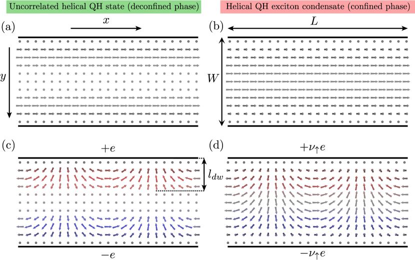
Figure 4: Spin textures. (a),(b) Ground state spin textures for the uncorrelated helical QH phase and the helical QH exciton condensate phase, respectively. In both cases there exists a robust domain wall, where the polar angle of the pseudospin magnetization $\theta(y)$ rotates from $\pi$ to $\theta_{b}$ along the $y$-direction. In the uncorrelated phase $\theta_{b}=0$ but in the helical QH exciton condensate phase $\theta_{b}\neq 0,\pi$ indicating spontaneous interlayer phase coherence in the bulk. In both cases the ground states are degenerate for all choices of the constant azimuthal angle $\phi$ of the pseudospin magnetization. (We have chosen $\phi=0$.) (c),(d) Charged excitations can be created by letting the azimuthal angle $\phi(x)$ to rotate along the $x$-direction. In a closed system (obtained by connecting the ends of the sample to form a narrow cylinder) $\phi(x)$ must rotate integer multiples of $2\pi$. The energy to create such kind of excitation in the uncorrelated helical QH phase scales as $\delta E\sim V_{2}^{XY}l_{dw}/L$, and the elementary excitations, which carry charge $\pm e$, can be created independently on the different edges. On the other hand, deep inside the helical QH exciton condensate phase $\delta E\sim V_{2}^{XY}W/L$ and the elementary charges are $\pm\nu_{\uparrow}e$. Furthermore, the charged edge excitations are confined: a charge $\pm\nu_{\uparrow}e$ on one of the edges is always connected to the opposite charge on the other edge by a stripe of rotated pseudospins through the bulk, and thus isolated charges cannot be observed at low energies. The charge density obtained from Eq. (4) is shown with red (positive charge density) and blue (negative charge density) colors.

The bulk gap for single particle excitations $E_{\rm gap,s}$ can be calculated using Hartree-Fock linearization supplementary

$$E_{\rm gap,s}=2\sqrt{(E_{Gb}-2V^{Z}_{0}h_{zb})^{2}+4(V^{XY}_{0})^{2}(h_{xb}^{2}+h_{yb}^{2})}.$$

Additionally to the single particle excitations, the helical QH exciton condensate supports collective excitations Moon et al. (1995): the neutral pseudospin waves (Goldstone mode) give rise to spin and counterflow charge superfluidity, and the lowest energy charged excitations are topological pseudospin textures, which carry fractional charge $\pm\nu_{\uparrow(\downarrow)}e$. Here $\nu_{\uparrow/\downarrow}=(1\pm h_{zb})/2$ are the pseudospin resolved filling factors of the different Landau levels. The energy required to create these charged excitations is slightly lower than $E_{\rm gap,s}$ Moon et al. (1995).

We point out that although $h_{zb}=\pm 1$ are topologically distinct phases, the bulk gap for creating charged excitations never closes, when one tunes from one phase to the other by controlling $E_{Gb}$. This is possible because the pseudospin rotation symmetry, which protects the existence of spin-resolved Chern numbers as topological numbers, is spontaneously broken in the helical exciton condensate phase. The interacting BHZ model for bilayers shows somewhat similar behavior also at zero magnetic field, where a trivial insulator phase can be connected to a quantum spin Hall insulator phase without closing of the bulk gap, because of an intermediate phase where the time-reversal symmetry is spontaneously broken Pikulin and Hyart (2014). It is also experimentally known that the exciton condensate phase with $\nu_{\uparrow}=\nu_{\downarrow}=1/2$ can be smoothly connected to uncorrelated QH state with $\nu_{\uparrow}=1$ and $\nu_{\downarrow}=0$ in conventional QH bilayers Ding . Experimental investigations of InAs/GaSb bilayers in the QH regime Du et al. (2013); Nichele14 are consistent with this prediction, because no gap closing has been observed as a function of magnetic field.

II Confinement-deconfinement transition of edge excitations

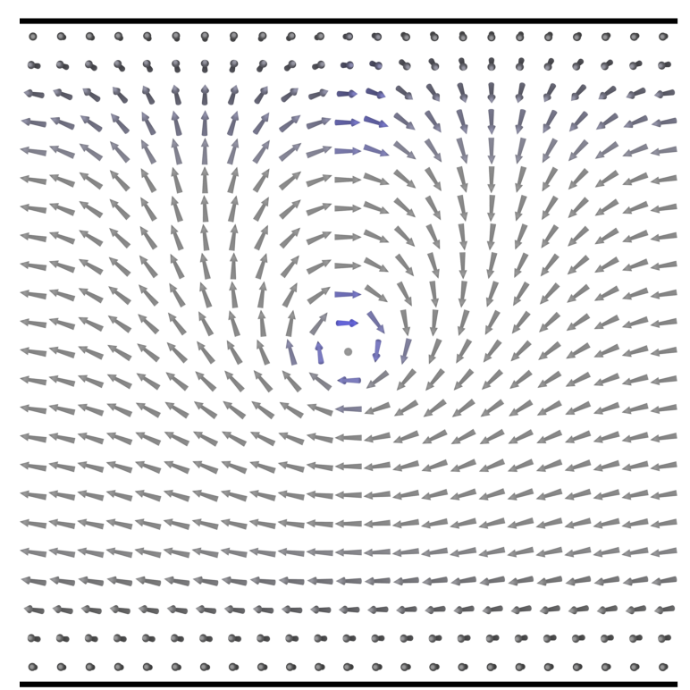
Figure 5: Charged excitation localized at one edge of the sample in the helical QH exciton condensate. The excitation can be visualized as a meron-antimeron pair, where the meron is localized inside the sample and anti-meron – outside. These excitations become the lowest energy charged excitations in sufficiently wide samples (otherwise similar cylinder geometry as in Fig. 4), where it is energetically favorable to break the stripe connecting opposite charges at the different edges by a creation of a bulk meron. Depending on the profile $E_{G}(y)$ near the edge, the lowest energy excitation is charge-neutral or having charge $\pm e$. The charge is determined by the pseudospin orientation in the center of the meron. The energy of such excitation is of order of Coulomb energy $V_{0}^{XY}$.

We now turn to the description of the ground state pseudospin texture $h_{z}(y)=\cos[\theta_{0}(y)]$, $h_{x}(y)=\sin[\theta_{0}(y)]\cos(\phi)$ and $h_{y}(y)=\sin[\theta_{0}(y)]\sin(\phi)$ at the edge. (The ground state will be degenerate with respect to the choice of $\phi$.) As discussed above close to the edge $E_{G}(y)>0$ takes large values, because the edge states are topologically protected to exist at all energies between the lowest Landau levels and higher ones. Therefore close to the edge $\theta_{0}(y)=\pi$. On the other hand, in the bulk $\theta_{0}(y)=\theta_{b}=\arccos(h_{zb})$. This means that there always exists a domain wall, where $\theta_{0}$ rotates from $\pi$ to $\theta_{b}$. Although the existence of the domain wall is a robust topological property of the system, the detailed shape of $\theta_{0}(y)$ and the length scale $l_{dw}$, where this rotation happens, depend on the details of the sample supplementary . The ground states in the uncorrelated helical QH phase ($\theta_{b}=0$) and helical QH exciton condensate phase ($\theta_{b}\neq 0,\pi$) are illustrated in Fig. 4 (a) and (b), respectively. It turns out that the existence of spontaneous interlayer phase coherence, which distinguishes the two different phases of matter, also has deep consequences on the nature of the low-energy excitations in this system.

By using a Hartree-Fock linearization for the ground state, we find that the single particle excitations are gapped also close to the edge, and the magnitude of the energy gap is determined by the Coulomb energy scale $V_{0}^{XY}$. However, similarly as for the case of a coherent domain wall in QH ferromagnetic state in graphene Fertig06 , the lowest energy edge excitations are not the single-particle ones. Namely, the ground state is degenerate with respect to the choice of $\phi$, and therefore in accordance with the Goldstone’s theorem the system supports low-energy excitations described by spatial variation of $\phi(\mathbf{r})$. Due to the general relationship between the electric and topological charge densities in QH ferromagnets Moon et al. (1995); supplementary ; Fertig06

$$\delta\rho(\mathbf{r})=-\frac{e}{4\pi}\frac{\partial\phi}{\partial x}\frac{\partial\cos[\theta_{0}(y)]}{\partial y}$$ (4)

these excitations also carry charge, which is localized at the edges of the sample. In this section we illustrate these excitations in a closed system obtained by connecting the ends of the sample to form a narrow cylinder with width $W$ and circumference $L$ comment3 .

We start by considering this kind of closed system, where $W\ll L$ (see Fig. 4). This geometry is topologically equivalent to a Corbino ring, which has been experimentally realized for QH exciton condensates Finck11 ; Xuting12 . Using Eqs. (LABEL:energyfunctional) and (4) we find that the lowest energy excitations correspond to rotation of $\phi(x)$ by $2\pi$ and carry a net charge within one of the edges supplementary . They have an energy $\delta E\sim V_{2}^{XY}l_{dw}/L$ in the uncorrelated phase and $\delta E\sim V_{2}^{XY}W/L$ deep in the helical exciton condensate phase. Here $V^{XY}_{2}=\frac{1}{2}\sum_{q}V_{P}^{XY}(q)q^{2}l_{B}^{2}$ characterizes the cost of exchange energy caused by $\nabla\phi(x)$ supplementary .

In the uncorrelated phase these excitations have a charge $\pm e$. By inspecting Fig. 4, we notice that because the spin points along $z$-direction in the bulk, there is no rotation happening in the bulk. This means that we can choose separate fields $\phi_{1}(x)$ and $\phi_{2}(x)$ for the two edges, so that these excitations can be created independently on the different edges much as in graphene Fertig06 .

The situation is dramatically different in the helical QH exciton condensate phase. There, the elementary excitations in a closed system have a charge $\pm\nu_{\uparrow}e$. Moreover, as illustrated in Fig. 4, a charge $\pm\nu_{\uparrow}e$ on one of the edges is always connected to the opposite charge on the other edge by a stripe of rotated bulk pseudospins. Breaking the bulk pseudospin configuration costs an energy comparable to the Coulomb energy, and thus isolated charges cannot be observed at low energies. This means that this type of charged edge excitations in the helical QH exciton condensate phase are confined.

It is illustrative to consider what happens to the excitations in the helical QH exciton condensate, when the width of the sample is increased. Namely, the excitation energy increases proportionally to the width of the sample $\delta E\sim V_{2}^{XY}W/L$ and eventually for $W\sim L$ it becomes energetically favorable instead of having a large area of rotating spins between two edges to create a bulk meron (see Fig. 5). This resembles the physics of quarks, where the growing separation of a quark-antiquark pair eventually results in the creation of a new quark-antiquark pair between them.

III Luttinger liquid theory and nonlocal transport

To predict experimentally measurable consequences of the charge confinement, we consider nonlocal transport in an open system. By considering the time-dependent field theory for the pseudospin for a reasonably narrow sample in the helical QH exciton condensate phase we arrive at an effective one-dimensional Hamiltonian supplementary

$$H=\int dx\bigg{[}\frac{e^{2}}{2W\hbar^{2}\Gamma}\Pi(x)^{2}+\frac{W\rho_{sb}}{2}(\partial_{x}\phi(x))^{2}\bigg{]},$$ (5)

where $\rho_{sb}=V^{XY}_{2}\sin^{2}\theta_{b}/\pi$ is the pseudospin stiffness and $\Gamma=e^{2}/(16\pi l_{B}^{2}(V_{0}^{XY}-V_{0}^{Z}))$ describes the interlayer capacitance per unit area, which is strongly enhanced from the electrostatic value by the exchange interactions. The one-dimensional charge densities in the different edges (labeled 1 and 2) $\rho_{1,2}(x)=\mp\frac{e}{4\pi}(1+\cos\theta_{b})\frac{\partial\phi}{\partial x}$ are always opposite and determined by a single field $\phi(x)$, highlighting the confinement of the charged edge excitations. The one-dimensional theory describes a Luttinger liquid, and the so-called Luttinger parameter $K$ in the convention used in Ref. Giamarchi , is given by

$$K=\frac{l_{B}}{W}\sqrt{\frac{V_{0}^{XY}-V_{0}^{Z}}{V_{2}^{XY}}}\frac{(1+\cos\theta_{b})^{2}}{4\sin\theta_{b}}.$$

The Luttinger parameter in quantum Hall systems determines the conductance for ideal contacts $G_{cf}=Ke^{2}/h$ Giamarchi ; KaneFisher . Because the pseudospin waves are charge neutral in the bulk, conductance decreases with $W$ as $G_{cf}\propto 1/W$. It is important to notice that in this system $G_{cf}$ describes the conductance for a counterflow/drag geometry, where opposite currents are flowing in the two edges. The helical QH exciton condensate phase does not support net transport current as long as the voltages $eV$ are small compared to $\hbar v\pi/W$ supplementary . This automatically leads to a remarkable transport property that characterizes the helical QH exciton condensate phase. Namely, by considering a nonlocal transport geometry shown in Fig. (6) (a), where a drive current is applied on one of the edges and a resulting drag current is measured on the opposite edge, we find that necessarily $I_{{\rm drag}}=I_{{\rm drive}}$ at small voltages. This should be contrasted to the uncorrelated helical phase, where the charged edge excitations are deconfined. In that case, one has two independent Luttinger liquid theories for the two edges supplementary , and therefore one expects only a weak drag current due to the Coulomb force acting between the charges. For $W\gg l_{B}$, we expect that this effect is negligible compared to drag current in the confined phase.

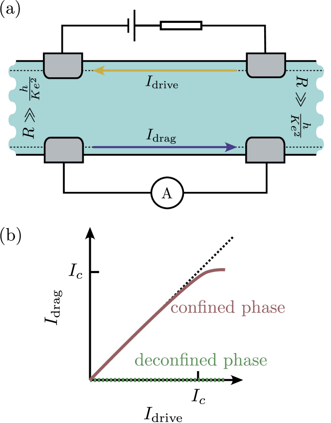
Figure 6: Nonlocal transport to demonstrate the charge confinement. (a) The transport geometry. A drive current is applied on one of the edges and the resulting drag current is measured on the opposite edge. (b) Due to the charge confinement in the helical QH exciton condensate phase, the drive current necessarily gives rises to an opposite drag current on the other edge. On the other hand, in the uncorrelated (deconfined) phase, there is only a weak drag current due to the Coulomb force acting between the charges.

Finally, to estimate the critical current $I_{c}$, where the relation $I_{{\rm drag}}=I_{{\rm drive}}$ breaks down, we notice that the maximum voltage is determined by the gap $eV_{max}\approx\hbar v\pi/W$. By using reasonable estimates $V_{0}^{Z}=V_{0}^{XY}/2$, $V_{2}^{XY}=V_{0}^{XY}/4$, $\theta_{b}=\pi/2$, $W=20l_{B}$, $l_{B}=10$ nm, $v=14$ km/s Spielman ; Hyart , we find $I_{c}=G_{cf}V_{max}\approx 0.1$ nA.

IV Summary and discussion

In summary, we have predicted the existence of a helical QH exciton condensate state in band-inverted electron-hole bilayers. We have shown that the counterpropagating edge modes give rise to a ground state pseudospin texture, where the polar angle of the pseudospin magnetization $\theta(y)$ rotates from the boundary value $\pi$ to the bulk value $\theta_{b}$ along the direction perpendicular to the edge. Low-energy charged excitations can be created by letting the azimuthal angle of the pseudospin polarization $\phi(x)$ to rotate along the edge. Remarkably, in a sufficiently narrow Hall bar these charged edge excitations are confined in the presence of spontaneous interlayer phase-coherence ($\theta_{b}\neq 0,\pi$): a charge on one of the edges always gives rise to the opposite charge on the other edge, and thus isolated charges cannot be observed at low energies. Moreover, we predict the possibility to control $\theta_{b}$ with a magnetic field and gate voltages. This allows to study a confinement-deconfinement transition, which occurs simultaneously with the bulk phase-transition between the helical QH exciton condensate phase ($\theta_{b}\neq 0,\pi$) and the uncorrelated helical QH phase ($\theta_{b}=0$).

The helical QH exciton condensate phase can be experimentally probed using Josephson-like interlayer tunneling and counterflow superfluidity Sarma and Pinczuk (2008); Girvin (1999); Eisenstein and MacDonald (2004); Moon et al. (1995); Finck11 ; Xuting12 ; Spielman ; Hyart . Moreover, because the pseudospin in this system describes simultaneously both the spin and the layer degrees of freedom, the helical QH exciton condensate phase can also be probed using the spin superfluidity and the NMR techniques Girvin (1999). Perhaps it is even possible to use local probe techniques to image the confinement-deconfinement transition and the confinement physics as illustrated in Figs. 4 and 5. Finally, we have shown that the charge confinement also gives rise to a remarkable new transport property. Namely, a drive current applied on one of the edges gives rise to exactly opposite drag current $I_{{\rm drag}}=I_{{\rm drive}}$ at the other edge.

Our results for the confinement of the edge excitations may also be applicable to the so-called canted antiferromagnetic phase, which is predicted to appear in graphene Murthy14 . Similarly to the helical QH exciton condensate state considered in this paper, the canted antiferromagnetic phase is characterized by a spontaneously broken U(1)-symmetry in the bulk and a single edge supports only gapped meron-antimeron excitations Murthy14 .

The phenomena of confinement stemming from the particle physics models Greensite (2011) has been studied also in condensed matter systems Volovik-book ; Volovik-review ; Helium-confinement-experiment ; Yang96 ; Lake10 . However, we expect that the combination of the different techniques for probing the helical QH exciton condensate phase will provide a more intuitive understanding and new perspectives on the confinement physics.

We also point out that InAs/GaSb bilayers is a promising system for superconducting applications, and edge-mode superconductivity has already been experimentally demonstrated in the QSH regime Pribiag . In the presence of superconducting contacts, the helical QH exciton condensate may provide a new route for realizing exotic nonlocal Josephson effects and non-Abelian excitations, such as parafermions Lindner et al. (2012); Clarke et al. (2013).

Acknowledgements.– This work was supported by the Academy of Finland Center of Excellence program, the European Research Council (Grant No. 240362-Heattronics), the Dutch Science Foundation NWO/FOM, NSERC, CIfAR, Max Planck - UBC Centre for Quantum Materials, and the DFG grant RE 2978/1-1.

Supplementary material for ”Confinement-deconfinement transition due to spontaneous symmetry breaking in quantum Hall bilayers”

Effective model from the BHZ Hamiltonian

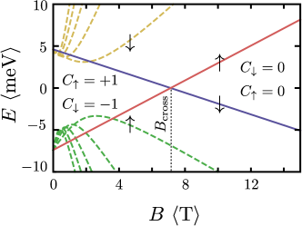
Figure 7: Landau level fan for the InAs/GaSb bilayer. The figure shows the energies of the lowest 6 Landau levels on each side of the Fermi level (in terms of the minimum of the absolute value of energy as a function of magnetic field) for the Hamiltonian (6) with characteristic values of the parameters for InAs/GaSb bilayers ${\cal{M}}=-6$ meV, ${\cal C}=-1.4$ meV, $\mathcal{B}=-78.3$ eVŲ, $\mathcal{D}=-18$ eVŲ and $\mathcal{A}=0.62$ eVÅ Liu and Zhang (2013). We have used the bulk values for the $g$-factors $g_{e}=-14.7$ and $g_{h}=-9.3$. For $B<B_{\rm cross}$ the spin-resolved Chern numbers are $C_{\uparrow}=-C_{\downarrow}=1$ (helical edge modes) whereas for $B>B_{\rm cross}$ the spin-resolved Chern numbers are $C_{\uparrow}=C_{\downarrow}=0$ (trivial insulator).

We consider bilayer QSH systems, such as InAs/GaSb bilayers, described by the BHZ Hamiltonian Bernevig et al. (2006); Liu et al. (2008)

$$H = \big{\{}{\cal{M}}-\mathcal{B}\big{[}(k_{x}-\frac{y}{l_{B}^{2}})^{2}+k_{y}^{2}\big{]}\big{\}}\sigma_{0}\tau_{z}+\mathcal{A}(k_{x}-\frac{y}{l_{B}^{2}})\sigma_{z}\tau_{x}-\mathcal{A}k_{y}\sigma_{0}\tau_{y}+\big{\{}{\cal C}-\mathcal{D}\big{[}(k_{x}-\frac{y}{l_{B}^{2}})^{2}+k_{y}^{2}\big{]}\big{\}}\sigma_{0}\tau_{0}$$ (6)

$$+\frac{g_{e}\mu_{B}B}{4}\sigma_{z}(\tau_{0}+\tau_{z})+\frac{g_{h}\mu_{B}B}{4}\sigma_{z}(\tau_{0}-\tau_{z}),$$

where $\sigma$ and $\tau$ are Pauli matrices in spin and electron-hole basis correspondingly, ${\cal{M}}$ describes the distance between the bottoms of electron and hole bands (in the inverted regime ${\cal{M}}<0$), ${\cal C}$ is the chemical potential, $\mathcal{B},\mathcal{D}<0$ ($|\mathcal{B}|>|\mathcal{D}|$) determine the effective masses for the electron and hole bands, $g_{e(h)}$ are the $g$-factors for electron and hole bands, respectively, and the magnetic field has been written in the Landau gauge with $l_{B}=\sqrt{\hbar/eB}$ being the magnetic length. This Hamiltonian describes an electron-hole bilayer, where the electron band in one of the layers is made out of $s$-orbitals and the hole band in the other layer is made out of $p$-orbitals, so that the tunneling between the layers (proportional to $\mathcal{A}$) is odd in momentum. There exist two strategies for constructing this kind of bilayer system. The first possibility is to use two different semiconducting materials where the $s$-like electron band in one of the materials and $p$-like hole band in the other material are inverted such as InAs/GaSb bilayers Liu et al. (2008); Du15_supp ; Spanton14_supp . The second strategy is to use in both layers the same semiconductor where the $s$-like electron band and the $p$-like hole band are close in energy, so that in a gated device one can reach a situation where the $s$-like electron band is active close to Fermi energy in one layer whereas the $p$-like hole band is active in the other. A promising approach to realize this possibility is to construct a bilayer in such a way that each layer individually supports the QSH effect Michetti_supp . Here we have neglected the spin-orbit coupling terms arising due to structural and bulk inversion asymmetry. In InAs/GaSb bilayers these terms are estimated to be very small Liu and Zhang (2013). The Landau level spectrum for InAs/GaSb bilayers is shown in Fig. 7. In this material the parameters of the model can be tuned with the help of gate voltages and widths of the quantum wells. Here we have used characteristic values of the parameters Liu and Zhang (2013) and the bulk values for the $g$-factors.

The two lowest Landau level wavefunctions for this model are

$$\psi_{k;\uparrow(\downarrow)}=\frac{e^{ikx}}{\sqrt{Ll_{B}}}\phi\left(\frac{y-kl_{B}^{2}}{l_{B}}\right)\begin{pmatrix}1(0)&0&0&0(1)\end{pmatrix}^{T},$$ (7)

where $\phi(\xi)=e^{-\xi^{2}/2}/\pi^{1/4}$. Notice that spin and orbital degrees of freedom are locked, so that the pseudospin $\uparrow$ ($\downarrow$) means simultaneously up (down) spin and upper (lower) layer. This locking is caused by the tunneling term proportional to $\cal{A}$, which is linear in momentum. Due to the existence of this term the electron-like Landau level with spin down (hole-like Landau level with spin up) couples to a hole-like (electron-like) higher Landau level, and as a result of this coupling these Landau levels are well separated in energy from the Landau levels given by Eq. (7). Within the subspace generated by these wave functions, the single-particle Hamiltonian is

$$\hat{H}_{0}=\sum_{k}[\hat{\psi}_{k,\uparrow}^{\dagger}\hat{\psi}_{k,\uparrow}-\hat{\psi}_{k,\downarrow}^{\dagger}\hat{\psi}_{k,\downarrow}]E_{G}(kl_{B}^{2}).$$ (8)

Here $\hat{\psi}_{k,\uparrow(\downarrow)}^{\dagger}$ and $\hat{\psi}_{k,\uparrow(\downarrow)}$ are the creation and annihilation operators corresponding to the electronic states described by Eq. (7), and we have fixed the chemical potential so that the total density corresponds to one of these Landau levels being filled and the other empty ($\nu_{T}=\nu_{\uparrow}+\nu_{\downarrow}=1$). The Fermi level is set to be at zero energy. For an infinite system in $y$-direction, the energy $E_{G}$ is independent on momentum and given by $E_{Gb}=\mathcal{M}-\frac{e\mathcal{B}}{\hbar}B+\frac{g_{e}+g_{h}}{4}\mu_{B}B$. Due to the presence of an edge the Landau levels obtain an energy-momentum dispersion. According to Eq. (7) the momentum is directly connected to the position $y$ in real space, so that this energy-momentum dispersion can also be written as a position-dependent energy $E_{G}(y)=E_{G}(kl_{B}^{2})$. The Landau level originating from the electron (hole) band always disperses upwards (downwards) in energy, when approaching the edge. Moreover, because the edge states exist at all energies between the lowest Landau levels and the higher ones, close to the edge $E_{G}(y)>0$ reaches extremely large values, which are on the same order as the energy separation between the bulk Landau levels. The spatial variation of $E_{G}(y)$ occurs within a characteristic length scale $l_{0}$, which for clean sharp edge is given by $l_{0}\sim l_{B}$. However, because the edge state velocity $v_{s}=\frac{1}{\hbar}\frac{dE_{G}}{dk}$ in the non-interacting theory is directly related to $l_{0}$, the edge roughness and disorder renormalize $l_{0}$ upwards ($v_{s}$ downwards), and hence $l_{0}$ can be considerably larger than $l_{B}$. The explicit form of the wave functions is given by Eq. (7) only if $l_{0}\gg l_{B}$, but our main results are expected to remain valid even if this condition is not satisfied.

Assuming that there is a band inversion at zero magnetic field (${\cal{M}},\mathcal{B}<0$), there is a crossing of the lowest Landau levels at magnetic field $B_{\rm cross}={\cal M}/(\frac{e{\cal B}}{\hbar}-\frac{g_{e}+g_{h}}{4}\mu_{B})$, where the band inversion is removed. For $B<B_{\rm cross}$, we notice that $E_{G}(y)=E_{Gb}<0$ in the bulk but $E_{G}(y)>0$ close to the edge, yielding helical edge states. On the other hand for $B>B_{\rm cross}$, $E_{G}(y)>0$ everywhere, and therefore the edge is gapped according to the non-interacting theory. The change in the edge structures shows up in the spin resolved Chern numbers. Namely for $B<B_{\rm cross}$ the spin-resolved Chern numbers are $C_{\uparrow}=-C_{\downarrow}=1$ (helical edge modes), whereas for $B>B_{\rm cross}$ $C_{\uparrow}=C_{\downarrow}=0$ (trivial insulator).

Energy functional

Within the subspace generated by the lowest Landau level wave functions, the projected Hamiltonian can be written as $\hat{H}=\hat{H}_{0}+\hat{H}_{I}$, where the interactions are described by

$$\hat{H}_{I}=\frac{1}{2}\sum_{\sigma,\sigma^{\prime}}\sum_{k,k^{\prime},q}V_{P}^{\sigma\sigma^{\prime}}(k-k^{\prime},q)\hat{\psi}_{k\sigma}^{\dagger}\hat{\psi}_{k^{\prime},\sigma^{\prime}}^{\dagger}\hat{\psi}_{k^{\prime}+q\sigma^{\prime}}\hat{\psi}_{k-q\sigma}.$$ (9)

Here, the projected Coulomb interactions can be written as

$$V_{P}^{\sigma\sigma^{\prime}}(k-k^{\prime},q)=\frac{\pi^{1/4}}{\sqrt{2}}\phi_{0}^{2}\bigg{(}\frac{ql_{B}}{\sqrt{2}}\bigg{)}\frac{1}{Ll_{B}}\int d^{2}r\ V^{\sigma\sigma^{\prime}}(\mathbf{r})e^{iqx}\phi_{0}\bigg{(}\frac{y-(k-k^{\prime}-q)l_{B}^{2}}{l_{B}}\bigg{)}.$$ (10)

To simplify the expressions we assume that the quantum wells are very narrow so that

$$V^{\uparrow\uparrow}(\mathbf{r})=V^{\downarrow\downarrow}(\mathbf{r})=\frac{e^{2}}{4\pi\epsilon\epsilon_{0}r},\hskip 14.22636ptV^{\uparrow\downarrow}(\mathbf{r})=V^{\downarrow\uparrow}(\mathbf{r})=\frac{e^{2}}{4\pi\epsilon\epsilon_{0}\sqrt{r^{2}+d^{2}}}.$$ (11)

This assumption does not change the results qualitatively. However, one should keep in mind that quantitatively the energy scales associated with the interaction effects are overestimated, because the finite width of the quantum well would reduce the effective interaction strengths.

To compute the energy for a pseudospin texture we follow closely the approach developed in Ref. Moon95_supp, . We assume that the components of the pseudospin $h_{i}(y)=h_{i}(kl_{B}^{2})$ are slowly varying with respect to $l_{B}$, so that we can express the many particle wave function as

$$|\Psi[\mathbf{h}(kl_{B}^{2})]\rangle=\prod_{k}\frac{1}{\sqrt{2[1-h_{z}(kl_{B}^{2})]}}\bigg{\{}\big{[}h_{x}(kl_{B}^{2})-ih_{y}(kl_{B}^{2})\big{]}\hat{\psi}_{k,\uparrow}^{\dagger}+\big{[}1-h_{z}(kl_{B}^{2})\big{]}\hat{\psi}_{k,\downarrow}^{\dagger}\bigg{\}}|0\rangle.$$ (12)

Here $\sum_{i}h_{i}^{2}(kl_{B}^{2})=1$. The energy functional can be obtained by calculating

$$E\big{[}\mathbf{h}(kl_{B}^{2})\big{]}=\langle\Psi\big{[}\mathbf{h}(kl_{B}^{2})\big{]}|\hat{H}_{0}+\hat{H}_{I}|\Psi\big{[}\mathbf{h}(kl_{B}^{2})\big{]}\rangle.$$ (13)

Using the Wick’s theorem, we obtain

$$E\big{[}\mathbf{h}(kl_{B}^{2})\big{]}=E_{0}+\sum_{k}E_{G}(kl_{B}^{2})h_{z}(kl_{B}^{2})-\sum_{k,k^{\prime}}\bigg{\{}V_{P}^{Z}(k-k^{\prime})h_{z}(kl_{B}^{2})h_{z}(k^{\prime}l_{B}^{2})+\sum_{i=x,y}V_{P}^{XY}(k-k^{\prime})h_{i}(kl_{B}^{2})h_{i}(k^{\prime}l_{B}^{2})\bigg{\}},$$ (14)

where

$$V^{Z}_{P}(q) = \frac{1}{4}\bigg{[}-V_{P}^{\uparrow\uparrow}(q,0)+V_{P}^{\uparrow\uparrow}(q,q)+V_{P}^{\uparrow\downarrow}(q,0)\bigg{]}=-\frac{V_{C}}{4\sqrt{2\pi}L}\int_{-\infty}^{\infty}dy\ln\bigg{[}\frac{y^{2}+d^{2}}{y^{2}}\bigg{]}e^{-(y/l_{B}-ql_{B})^{2}/2}$$ (15)

$$+\frac{V_{C}}{4\sqrt{2\pi}L}e^{-q^{2}l_{B}^{2}/2}\int_{-\infty}^{\infty}dx\ e^{iqx}e^{x^{2}/4l_{B}^{2}}K_{0}\bigg{(}\frac{x^{2}}{4l_{B}^{2}}\bigg{)}$$

and

$$V_{P}^{XY}(q)=\frac{1}{4}V_{P}^{\uparrow\downarrow}(q,q)=\frac{e^{-q^{2}l_{B}^{2}/2}V_{C}}{4\sqrt{2\pi}L}\int_{-\infty}^{\infty}dx\ e^{iqx}e^{x^{2}/4l_{B}^{2}+d^{2}/4l_{B}^{2}}K_{0}\bigg{(}\frac{x^{2}+d^{2}}{4l_{B}^{2}}\bigg{)}.$$ (16)

Here the characteristic energy scale of the Coulomb interactions is $V_{C}=e^{2}/(4\pi\epsilon\epsilon_{0}l_{B})$.

Mean field solutions in the bulk

Before describing the pseudospin texture at the edge, let’s solve the ground state orientation of the pseudospin in the bulk. By assuming a homogeneous solution in the bulk, we obtain

$$E[\mathbf{h}] = E_{0}+\frac{L^{2}}{2\pi l_{B}^{2}}\bigg{[}E_{Gb}h_{z}-V^{Z}_{0}h_{z}^{2}-V^{XY}_{0}(h_{x}^{2}+h_{y}^{2})\bigg{]},$$ (17)

where $E_{Gb}$ is the bulk value of $E_{G}(y)$ (in the inverted regime $E_{Gb}<0$ and in the non-inverted regime $E_{Gb}>0$),

$$V^{Z}_{0}=\sum_{q}V_{P}^{Z}(q)=V_{C}\frac{1}{4}\bigg{[}\sqrt{\frac{\pi}{2}}-\frac{d}{l_{B}}\bigg{]}$$ (18)

and

$$V^{XY}_{0}=\sum_{q}V_{P}^{XY}(q)=V_{C}\frac{1}{4}\sqrt{\frac{\pi}{2}}e^{d^{2}/2l_{B}^{2}}\textrm{Erfc}\bigg{[}\frac{d}{\sqrt{2}l_{B}}\bigg{]}.$$ (19)

By minimizing the energy given Eq. (17) with a constraint $\sum_{i}h_{i}^{2}=1$, we obtain

$$h_{zb}=\begin{cases}1,&-\frac{E_{Gb}}{2(V^{XY}_{0}-V^{Z}_{0})}>1\\ -\frac{E_{Gb}}{2(V^{XY}_{0}-V^{Z}_{0})},&\big{|}\frac{E_{Gb}}{2(V^{XY}_{0}-V^{Z}_{0})}\big{|}<1\\ -1,&-\frac{E_{Gb}}{2(V^{XY}_{0}-V^{Z}_{0})}<-1\\ \end{cases}$$ (20)

The other components satisfy $h_{xb}^{2}+h_{yb}^{2}=1-h_{zb}^{2}$ and the energy is degenerate with respect to the rotations in the $(x,y)$-plane.

To estimate the single particle excitation gap in the bulk, we can construct a mean field Hamiltonian by Hartree-Fock linearization of the interaction terms. This way we obtain

$$\hat{H}_{\rm mf}=\sum_{k}(\hat{\psi}_{k,\uparrow}^{\dagger},\hat{\psi}_{k,\downarrow}^{\dagger})\begin{pmatrix}E_{Gb}+m_{zb}&m_{xb}-im_{yb}\\ m_{xb}+im_{yb}&-E_{Gb}-m_{zb}\end{pmatrix}\begin{pmatrix}\hat{\psi}_{k,\uparrow}\\ \hat{\psi}_{k,\downarrow}\end{pmatrix},$$ (21)

where $m_{zb}=-2V^{Z}_{0}h_{zb}$, $m_{xb}=-2V^{XY}_{0}h_{xb}$ and $m_{yb}=-2V^{XY}_{0}h_{yb}$. The bulk gap for single particle excitations is thus

$$E_{\rm gap,s}=2\sqrt{(E_{Gb}-2V^{Z}_{0}h_{zb})^{2}+4(V^{XY}_{0})^{2}(h_{xb}^{2}+h_{yb}^{2})}.$$ (22)

In addition to the crossing of the Landau levels as a function of magnetic field, several other conditions need to be satisfied in order to realize the helical exciton condensate phase: (i) The other Landau levels at the crossing point are separated in energy so that they are not excited. (ii) The densities close to the charge neutrality point can be obtained so that $\nu_{\uparrow}$ and $\nu_{\downarrow}$ can be controlled with magnetic field and gate voltages. (iii) The layer separation described by $d/l_{B}$ can be made sufficiently small to reach the exciton condensate phase. (iv) The temperature can be made small enough to reach the exciton condensate phase. (v) The disorder should not be too strong.

(i) As demonstrated in Fig. 7 the typical energy gap to higher Landau levels in InAs/GaSb bilayers is on the order of $10$ meV, which is significantly larger than the gap opened by the exciton condensate order parameter. We also point out that although the large gap to higher Landau levels simplifies the theoretical analysis, it may not be necessary for the existence of exciton condensate state because the interaction effects actually tend to enhance this energy gap further. In fact, in GaAs bilayers the lowest Landau levels are separated from the higher ones by the Zeeman energy which is a rather small energy scale, but nevertheless the spin is fully polarized in the exciton condensate state Spielman-spin ; Giudici ; Finck10 ; Tiemann15 .

(ii) In InAs/GaSb bilayers the densities close to the charge neutrality point can be experimentally reached in gated devices both in the absence Du15_supp ; Spanton14_supp ; Qu15_supp ; Du15EC_supp and in the presence Nichele14_supp of the magnetic field.

(iii) In GaAs quantum Hall bilayers it is known that the exciton condensate phase appears for $d/l_{B}\lesssim 1.8$ Murphy94_supp ; Spielman00_supp ; Kellogg02_supp ; Champagne08_supp ; Tiemann09_supp . Using the typical parameters of the experimental samples Du15_supp ; Spanton14_supp ; Qu15_supp we find that this condition can be easily satisfied in InAs/GaSb bilayers.

(iv) The temperature needs to be smaller than the energy gap opened by the exciton condensate order parameter. Moreover, since we are studying a two dimensional system the actual transition to the exciton condensate phase is a Berezinskii-Kosterlitz-Thouless transition Moon95_supp , and the transition temperature can be estimated to be on the order of Kelvin. The transition temperatures measured in GaAs bilayers are consistent with this type of estimate Champagne08_supp .

(v) The mean free path should be long compared to the coherence length. In quantum Hall exciton condensates the coherence length is on the order of $l_{B}$ and therefore this condition is easily satisfied. However, the disorder plays also another role in this system. Namely, the vortices are charged and therefore they can be nucleated by a sufficiently strong disorder potential Eastham09_supp ; Sun10_supp . Although the detailed consideration of the disorder is not the subject of this paper, we point out that most of the phenomenology of the quantum Hall exciton condensate state survives at least approximately also in the presence of the disorder-nucleated vortices Stern11_supp ; Fertig05_supp ; Eastham10_supp ; Hyart11_supp ; Hyart13_supp .

Domain wall at the edge

In order to describe the domain wall at the edge we first write $h_{z}(kl_{B}^{2})=\cos[\theta(kl_{B}^{2})]$, $h_{x}(kl_{B}^{2})=\sin[\theta(kl_{B}^{2})]$ and $h_{y}(kl_{B}^{2})=0$. [There is a degeneracy in ($h_{x},h_{y}$)-plane, so that we can choose a specific direction arbitrarily.] The energy functional [Eq. (14)] can then be written as

$$E\big{[}\theta(kl_{B}^{2})\big{]}=\sum_{k}E_{G}(kl_{B}^{2})\cos[\theta(kl_{B}^{2})]-\sum_{k,k^{\prime}}\bigg{\{}V_{P}^{Z}(k-k^{\prime})\cos[\theta(kl_{B}^{2})]\cos[\theta(k^{\prime}l_{B}^{2})]+V_{P}^{XY}(k-k^{\prime})\sin[\theta(kl_{B}^{2})]\sin[\theta(k^{\prime}l_{B}^{2})]\bigg{\}}.$$ (23)

By minimizing this with respect to $\theta(kl_{B}^{2})$, we obtain

$$\tan(\theta(kl_{B}^{2}))=\frac{2\sum_{k^{\prime}}V_{P}^{XY}(k-k^{\prime})\sin[\theta(k^{\prime}l_{B}^{2})]}{2\sum_{k^{\prime}}V_{P}^{Z}(k-k^{\prime})\cos[\theta(k^{\prime}l_{B}^{2})]-E_{G}(kl_{B}^{2})}.$$ (24)

This can be solved numerically by iterations.

Close to the edge $E_{G}(y)>0$ takes large values, because the edge states are topologically protected to exist at all energies between the lowest Landau levels and higher ones. Therefore close to the edge $\theta(y)=\pi$. On the other hand, in the bulk $\theta(y)=\theta_{b}=\arccos(h_{zb})$. This means the existence of a domain wall, where $\theta$ rotates from $\pi$ to $\theta_{b}$, is a robust topological property of the system, which is not sensitive to the details of the sample.

The width of the domain wall is $l_{dw}\sim{\rm{max}}\{l_{s},l_{0}\}$, where $l_{0}$ is the length scale where $E_{G}(y)$ changes in the vicinity of the edge and $l_{s}$ is an intrinsic length scale, which is determined by the balance between the energy gain obtained by rotating $\theta$ and the corresponding loss of the exchange energy. A rough estimate is obtained by expanding Eq. (17) around $\theta_{b}$ and noticing that the loss of exchange energy is approximately determined by (see Section Charged edge excitations)

$$V^{XY}_{2}=\frac{1}{2}\sum_{q}V_{P}^{XY}(q)q^{2}l_{B}^{2}=V_{C}\frac{1}{16}\sqrt{\frac{\pi}{2}}e^{d^{2}/2l_{B}^{2}}\textrm{Erfc}\bigg{[}\frac{d}{\sqrt{2}l_{B}}\bigg{]}.$$ (25)

This leads to a simple estimate

$$l_{s}\approx\sqrt{\frac{2V_{2}^{XY}}{2(V_{0}^{XY}-V_{0}^{Z})(1-2h_{zb}^{2})-E_{Gb}h_{zb}}}l_{B}.$$ (26)

This length scale $l_{s}$ diverges at the phase transitions $h_{z}=1$, $E_{Gb}=-2(V_{0}^{XY}-V_{0}^{Z})$ and $h_{z}=-1$, $E_{Gb}=2(V_{0}^{XY}-V_{0}^{Z})$ indicating that $\theta(y)$ approaches the bulk value in a power-law like fashion (outside the phase transitions it approaches the bulk value exponentially). Deep inside the helical quantum Hall exciton condensate phase $l_{s}\sim l_{B}$.

Charged edge excitations

We now consider excitations $h_{z}(\mathbf{r})=h_{z}^{0}(y)+\delta h_{z}(\mathbf{r})$, $h_{x}(\mathbf{r})=\sqrt{1-h_{z}^{2}(\mathbf{r})}\cos[\phi(\mathbf{r})]$ and $h_{y}(\mathbf{r})=\sqrt{1-h_{z}^{2}(\mathbf{r})}\sin[\phi(\mathbf{r})]$, which are described by slow spatial variation of the pseudospin within the $(x,y)$-plane [$\phi(\mathbf{r})$] and small fluctuations [$\delta h_{z}(\mathbf{r})$] of the $z$-component around the ground state configuration $h_{z}^{0}(y)=\cos[\theta_{0}(y)]$.

For this purpose, we first write Eq. (14)

$$E\big{[}\mathbf{h}(kl_{B}^{2})\big{]}=E_{0}[h_{z}(kl_{B}^{2})]-\sum_{k,k^{\prime}}\bigg{\{}\sum_{i=x,y}V_{P}^{XY}(k-k^{\prime})h_{i}(kl_{B}^{2})h_{i}(k^{\prime}l_{B}^{2})\bigg{\}}.$$ (27)

By expanding ($i=x,y$)

$$h_{i}(kl_{B}^{2})h_{i}(k^{\prime}l_{B}^{2})=h_{i}^{2}(kl_{B}^{2})+h_{i}(kl_{B}^{2})(k^{\prime}l_{B}^{2}-kl_{B}^{2})h^{\prime}_{i}(kl_{B}^{2})+\frac{1}{2}h_{i}(kl_{B}^{2})(k^{\prime}l_{B}^{2}-kl_{B}^{2})^{2}h^{\prime\prime}_{i}(kl_{B}^{2})...$$ (28)

we obtain

$$E\big{[}\mathbf{h}\big{]} = E_{0}[h_{z}]-\frac{L}{2\pi l_{B}^{2}}\int dy\bigg{\{}V^{XY}_{0}\sum_{i=x,y}h_{i}^{2}(y)+V^{XY}_{2}l_{B}^{2}\sum_{i=x,y}h_{i}(y)h^{\prime\prime}_{i}(y)\bigg{\}}$$ (29)

$$= E_{0}[h_{z}]-\frac{1}{2\pi l_{B}^{2}}\int d^{2}r\bigg{\{}V^{XY}_{0}\sum_{i=x,y}h_{i}^{2}(\mathbf{r})+V^{XY}_{2}l_{B}^{2}\sum_{i=x,y}h_{i}(\mathbf{r})\nabla^{2}h_{x}(\mathbf{r})\bigg{\}}$$

$$= E_{0}[h_{z}]+\frac{1}{2\pi l_{B}^{2}}\int d^{2}r\bigg{\{}V^{XY}_{2}l_{B}^{2}\sum_{i=x,y}\big{[}\nabla h_{i}(\mathbf{r})\big{]}^{2}-V^{XY}_{0}\sum_{i=x,y}h_{i}^{2}(\mathbf{r})\bigg{\}}.$$

Here, we have transformed from momentum space $k$ to real space $y$ by using $y=kl_{B}^{2}$, restored the possibility that $\mathbf{h}(\mathbf{r})$ may also vary in the $x$-direction (using rotational symmetry of the system), assumed a boundary condition

$$\int d^{2}r\ \nabla\cdot(h_{i}\nabla h_{i})=0$$ (30)

and $V^{XY}_{2}$ is given by Eq. (25).

Similar gradient expansion cannot be done for $h_{z}(\mathbf{r})$ because of the long-range Hartree interactions. However, deep inside the phases $\delta h_{z}(\mathbf{r})$ mode is gapped by a large energy gap, and therefore we assume that as a first approximation it is enough to take the Hartree interactions into account only via the $V_{0}^{Z}$ term. In order to calculate the excitation energy we define a functional

$$E\big{[}\mathbf{h},\lambda\big{]}=E\big{[}\mathbf{h}\big{]}+\frac{1}{2\pi l_{B}^{2}}\int d^{2}r\ \lambda(\mathbf{r})(1-\sum_{i}h_{i}(\mathbf{r})^{2}),$$ (31)

where we have now explicitly implemented the constraint $\sum_{i}h_{i}^{2}=1$ with the help of Lagrange multiplier. The minimization of $E\big{[}\mathbf{h},\lambda\big{]}$ with respect to all variables leads to a saddle point equation (24) and allows us to consider fluctuations $\delta h_{i}(\mathbf{r})$ around the saddle point independently on each other. For general $E_{G}(y)$ the saddle point equation can be solved only numerically. Here we proceed by assuming that $E_{G}(y)$ is slowly varying. This is always satisfied in the bulk and we will comment the influence of the edge corrections below.

With these approximation the excitation energy (energy difference compared to the ground state) can be written as

$$\delta E\big{[}\delta h_{z}(\mathbf{r}),\phi(\mathbf{r})\big{]}=\frac{1}{2\pi l_{B}^{2}}\int d^{2}r\bigg{\{}V^{XY}_{2}l_{B}^{2}\sin^{2}[\theta_{0}(y)]\big{[}\nabla\phi(\mathbf{r})\big{]}^{2}+\bigg{[}(V_{0}^{XY}-V_{0}^{Z})\sin^{2}[\theta_{0}(y)]-\frac{E_{G}(y)}{2}\cos[\theta_{0}(y)]\bigg{]}\delta h_{z}^{2}(\mathbf{r})\bigg{\}}.$$ (32)

A variational wave function describing a general pseudospin texture $\mathbf{h}(\mathbf{r})$ is no longer restricted to the lowest Landau level. Therefore, the many particle wave function needs to be projected to the lowest Landau level with an operator $\cal{P}$, which can be implemented as explained in Ref. Moon95_supp, . This results in a charge density for such kind of excitations, which can be computed from the general relationship between the electric and topological charge densities Moon95_supp

$$\delta\rho(\mathbf{r})=-\frac{e}{8\pi}\epsilon_{\mu\nu}\mathbf{h}(\mathbf{r})\cdot[\partial_{\mu}\mathbf{h}(\mathbf{r})\times\partial_{\nu}\mathbf{h}(\mathbf{r})].$$ (33)

For the low-energy excitations, the charge density is therefore (see also Section Spin texture-charge density relation in quantum Hall systems and numerical calculation of the electric charge density for the spin textures)

$$\delta\rho(\mathbf{r})=-\frac{e}{4\pi}\frac{\partial\phi}{\partial x}\frac{\partial\cos[\theta_{0}(y)]}{\partial y}.$$ (34)

From this expression we see that the charge density is localized in the vicinity of the edge, and the length scale in $y$-direction is determined by the domain wall width $l_{dw}$. Moreover, the low-energy charged excitations are always associated with spatial variation of $\phi$ along the edge, so that the charge density is proportional to $\partial_{x}\phi$. We will study the nature of these excitations separately in the two opposite limits $E_{Gb}\ll-2(V^{XY}_{0}-V^{Z}_{0})$ (deep inside the uncorrelated helical quantum Hall state) and $|E_{Gb}|\ll 2(V^{XY}_{0}-V^{Z}_{0})$ (deep inside the helical quantum Hall exciton condensate phase).

Charged edge excitations in a closed system

We consider narrow quantum Hall systems with width $W$ much smaller than the length $L$ (similarly as shown in Fig. 4 in the main text), and we assume that the system is closed by connecting the ends of the sample. Based on Eqs. (32) and (34) we argue that the lowest energy charged excitations are obtained by letting azimuthal angle $\phi(x)$ rotate along the $x$-direction. In a closed system the angle $\phi(x)$ needs to rotate integer multiple of $2\pi$. The lowest energy excitations in a closed system, which carry a net charge within one of the edges correspond to rotation of $\phi(x)$ by $2\pi$, and they have an energy $\delta E\sim V_{2}^{XY}l_{dw}/L$ deep inside the uncorrelated phase and $\delta E\sim V_{2}^{XY}W/L$ deep inside the helical exciton condensate phase.

In the uncorrelated phase we obtain from Eq. (34) that these excitations have a charge $\pm e$. Moreover, they are deconfined: One can create these excitations independently on the different edges.

In the helical quantum Hall exciton condensate phase, we obtain from Eq. (34), that the elementary excitations in a closed system have a charge is $\pm\nu_{\uparrow}e$, where $\nu_{\uparrow}=(1+\cos\theta_{b})/2$. Moreover, a charge $\pm\nu_{\uparrow}e$ on one of the edges is always connected to the opposite charge on the other edge by a stripe of rotated pseuspins through the bulk. Creating this stripe costs an energy $\delta E\sim V_{2}^{XY}W/L$, which is proportional to the distance $W$ between the charges. However, breaking the stripe somewhere in the bulk would cost a much larger energy comparable to the Coulomb energy. Thus isolated charges cannot be observed at low energies. This means that in the helical quantum Hall exciton condensate phase the charged edge excitations are confined.

Luttinger liquid theory

To develop time-dependent theory for these excitations, we use the known result that the Euclidian action in the adiabatic approximation can be written as Moon95_supp

$$S^{E}[\mathbf{h},\lambda]=\int_{0}^{\beta}d\tau\bigg{\{}\int d^{2}r\bigg{[}-i\frac{1}{4\pi l_{B}^{2}}\mathbf{A}(\mathbf{h})\cdot\partial_{\tau}\mathbf{h}\bigg{]}+E\big{[}\mathbf{h},\lambda\big{]}\bigg{\}},$$ (35)

where $\nabla_{\mathbf{h}}\times\mathbf{A}(\mathbf{h})=\mathbf{h}$. Thus by assuming that $E_{G}(y)$ is slowly varying function, we can expand the action around the saddle point and obtain

$$\delta S^{E}[\phi,\delta h_{z}]=\frac{1}{2\pi l_{B}^{2}}\int_{0}^{\beta}d\tau\int d^{2}r\bigg{\{} \frac{i}{2}\delta h_{z}\frac{\partial\phi}{\partial\tau}+V_{2}^{XY}l_{B}^{2}\sin^{2}\theta_{0}+\bigg{[}(V_{0}^{XY}-V_{0}^{Z})\sin^{2}\theta_{0}(y)-\frac{E_{G}(y)}{2}\cos\theta_{0}(y)\bigg{]}\delta h_{z}^{2}\bigg{\}}.$$ (36)

.1 Confined phase

Deep inside the confined phase, all the properties of the system will be determined by the bulk (see below). Therefore, we neglect the effects arising in the vicinity of the edge, and use Eq. (20) to rewrite the action as

$$\delta S^{E}[\phi,\delta h_{z}]=\frac{1}{2\pi l_{B}^{2}}\int_{0}^{\beta}d\tau\int d^{2}r\bigg{\{} \frac{i}{2}\delta h_{z}\frac{\partial\phi}{\partial\tau}+V_{2}^{XY}l_{B}^{2}\sin^{2}\theta_{0}+(V_{0}^{XY}-V_{0}^{Z})\delta h_{z}^{2}\bigg{\}}$$ (37)

We integrate out the massive fluctuations $\delta h_{z}$. This way we obtain

$$S^{E}\big{[}\phi(\mathbf{r},\tau)\big{]}=\frac{1}{2\pi l_{B}^{2}}\int_{0}^{\beta}d\tau\int d^{2}r\bigg{\{}\frac{(\partial_{\tau}\phi)^{2}}{16(V_{0}^{XY}-V_{0}^{Z})}+V^{XY}_{2}l_{B}^{2}\sin^{2}[\theta_{0}(y)]\big{[}\nabla\phi(\mathbf{r})\big{]}^{2}\bigg{\}}.$$ (38)

By going to real time, we identify the Langrangian density as

$$\mathcal{L}=\frac{\hbar^{2}\Gamma}{2e^{2}}\dot{\phi}^{2}-\frac{\rho_{s}(y)}{2}(\nabla\phi)^{2}.$$ (39)

Here $\rho_{s}(y)=V^{XY}_{2}\sin^{2}[\theta_{0}(y)]/\pi$ is the pseudospin stiffness and $\Gamma=e^{2}/(16\pi l_{B}^{2}(V_{0}^{XY}-V_{0}^{Z}))$ describes the interlayer capacitance per unit area, which is strongly enhanced from the electrostatic value by the exchange interactions. (As an important check we notice that if one neglects the exchange contributions in $V_{0}^{XY}-V_{0}^{Z}$, the expression for $\Gamma$ simplifies to the familiar electrostatic formula for the interlayer capacitance.)

The corresponding equation of motion is

$$\frac{\hbar^{2}\Gamma}{e^{2}}\ddot{\phi}-\nabla\left[\rho_{s}(y)\nabla\phi\right]=0.$$ (40)

This equation is translationary invariant in $x$ and $t$ thus we can express the solution as

$$\phi=\phi_{0}+\sum_{n,k}e^{-i[\omega_{n}(k)t-kx]}f_{n,k}(y),$$ (41)

where $\phi_{0}$ is an arbitrary constant and $f_{n,k}(y)$ describe the different transverse modes with energy-momentum dispersions $E_{n}(k)=\hbar\omega_{n}(k)$. By substituting the trial solution (41) to Eq. (40), we find that the eigenfunctions $f_{n,k}(y)$ and eigenfrequencies $\omega_{n}(k)$ satisfy an eigenvalue equation

$$-\frac{\hbar^{2}\Gamma\omega_{n}(k)^{2}}{e^{2}}f_{n,k}(y)+k^{2}\rho_{s}(y)f_{n,k}(y)-\rho_{s}(y)f_{n,k}^{\prime\prime}(y)-\rho_{s}^{\prime}(y)f_{n,k}^{\prime}(y)=0,$$ (42)

which can be solved numerically.

Numerical results for the helical quantum Hall exciton condensate phase show that the lowest energy mode $f_{0,k}(y)$ can be approximated as a constant throughout the sample. Moreover, the lowest energy mode at reasonably small momentum is separated from higher modes by an energy $\Delta E\sim\hbar v\pi/W$. We restrict the analysis to sufficiently low-energies that these higher modes are not excited. Then we assume that $\phi$ is constant in $y$-direction and the dispersion relation is

$$\omega(k)=\sqrt{\frac{e^{2}\rho_{sb}}{\hbar^{2}\Gamma}}k=vk,$$ (43)

where $\rho_{sb}$ is the bulk value of $\rho_{s}(y)$. The Hamiltonian of the system then becomes

$$H=\int dx\bigg{[}\frac{e^{2}}{2W\hbar^{2}\Gamma}\Pi(x)^{2}+\frac{W\rho_{sb}}{2}(\partial_{x}\phi(x))^{2}\bigg{]},$$ (44)

where $\Pi(x)$ is the momentum conjugate to $\phi(x)$. The one-dimensional charge densities in the different edges (labelled 1 and 2) are

$$\rho_{1,2}(x)=\mp\frac{e}{4\pi}(1+\cos\theta_{b})\frac{\partial\phi}{\partial x},$$ (45)

where $\theta_{b}$ is the bulk value of $\theta(y)$. The confinement of the edge excitation clearly shows up here as the the charge densities on the different edges are always opposite and determined by a single field $\phi(x)$. This Hamiltonian describes a Luttinger liquid. In the standard convention Giamarchi_supp the Luttinger liquid theory is written as

$$H=\frac{\hbar}{2\pi}\int dx\bigg{[}\frac{vK\pi^{2}}{\hbar^{2}}\tilde{\Pi}(x)^{2}+\frac{v}{K}(\partial_{x}\tilde{\phi})^{2}\bigg{]},\hskip 14.22636pt\rho(x)=-\frac{e}{\pi}\frac{\partial\tilde{\phi}}{\partial x}.$$ (46)

To rewrite our Hamiltonian in this convention, we apply the transformation preserving canonical commutation relations

$$\phi(x)=\frac{4}{1+\cos\theta_{b}}\tilde{\phi}(x),\hskip 14.22636pt\Pi(x)=\frac{1+\cos\theta_{b}}{4}\tilde{\Pi}(x),$$ (47)

and notice that the charge density at each edge is $\rho_{1,2}(x)=\pm\rho(x)$.

This way, we can identify the Luttinger liquid parameters $K$ and $v$ as

$$v=\sqrt{\frac{e^{2}\rho_{sb}}{\hbar^{2}\Gamma}},\hskip 14.22636ptK=\frac{e}{\pi W\sqrt{\Gamma\rho_{sb}}}\bigg{(}\frac{1+\cos\theta_{b}}{4}\bigg{)}^{2}=\frac{l_{B}}{W}\sqrt{\frac{V_{0}^{XY}-V_{0}^{Z}}{V_{2}^{XY}}}\frac{(1+\cos\theta_{b})^{2}}{4\sin\theta_{b}}.$$ (48)

Here, $v$ is just the pseudospin wave velocity obtained earlier from the dispersion $\omega(k)$. The Luttinger parameter $K$ determines the conductance $G_{cf}=Ke^{2}/h$. However, it is important to notice that $G_{cf}$ describes the conductance for a counterflow/drag geometry, where opposite currents are flowing in the two edges. The helical quantum Hall exciton condensate phase does not support net transport current as long as the voltages $eV$ are small compared to $\hbar v\pi/W$.

.2 Deconfined phase

In the uncorrelated helical quantum Hall phase the transverse modes are localized within the length scale $l_{dw}$ from the edges. Therefore, in contrast to helical quantum Hall exciton condensate phase we can define independent fields $\phi_{1(2)}(x)$ and charge densities $\rho_{1(2)}(x)=\mp\frac{e}{2\pi}\frac{\partial\phi_{1(2)}}{\partial x}$. Thus charges can be created independently on the different edges, highlighting that in the uncorrelated helical phase the charged edge excitations are deconfined.

We can now repeat the calculation done above for the confined phase. This way, assuming that $E_{G}(y)$ is slowly varying and that the transverse modes are described by a constant within a distance $l_{dw}$ in the vicinity of the edge and $0$ elsewhere, we arrive to Luttinger liquid Hamiltonian

$$H=\sum_{i=1}^{2}\int dx\bigg{[}\frac{e^{2}}{2l_{dw}\hbar^{2}\Gamma_{av}}\Pi_{i}(x)^{2}+\frac{l_{dw}\rho_{s,av}}{2}(\partial_{x}\phi_{i}(x))^{2}\bigg{]},$$ (49)

where $\rho_{s,av}=\frac{1}{l_{dw}}\int_{0}^{l_{dw}}dy\ V^{XY}_{2}\sin^{2}[\theta_{0}(y)]/\pi$ and $\Gamma_{av}=\frac{1}{l_{dw}}\int_{0}^{l_{dw}}dy\ e^{2}/\{16\pi l_{B}^{2}[(V_{0}^{XY}-V_{0}^{Z})\sin^{2}\theta_{0}(y)-\frac{E_{G}(y)}{2}\cos\theta_{0}(y)]\}$. This way the Luttinger liquid parameters are identified as

$$v=\sqrt{\frac{e^{2}\rho_{s,av}}{\hbar^{2}\Gamma_{av}}},\hskip 14.22636ptK=\frac{e}{4\pi l_{dw}\sqrt{\Gamma_{av}\rho_{s,av}}}.$$ (50)

However, in contrast to the helical quantum Hall exciton condensate phase the Luttinger liquid parameters depend strongly on the detailed shape of the $E_{G}(y)$ function, and if it is not slowly varying in the vicinity of the edge, there can be large corrections to the expressions above. Nevertheless, the structure of the Luttinger liquid theory (49) is very general, and for physically reasonable parameters $K\sim 1$. Thus we expect this phase to support helical edge state transport with conductance $G\sim e^{2}/h$. Here $G$ describes the conductance for a transport geometry, where a net transport current is flowing along one of the edges.

Spin texture-charge density relation in quantum Hall systems and numerical calculation of the electric charge density for the spin textures

It is known that both topological and non-topological contributions to the electric charge exist at the vortices in various systems Khomskii ; Blatter ; Kumagai ; Natsik ; Shevc ; Volovik ; Rukin ; Adamenko . It is possible to show that the mechanisms considered in these systems do not give rise to a non-topological contribution to the electric charge in quantum Hall exciton condensates. However, instead of going through the mechanisms one-by-one, we present general arguments for the topological spin texture-charge density relation and discuss the conditions for its breakdown. We complement the analytical arguments with a numerical calculation of the electric charge density for the pseudospin textures considered in the paper.

Originally the spin texture-charge density relation for quantum Hall systems was argued from the Chern-Simons relation between the density and the statistical magnetic field Sondhi93_supp . Namely, the electrons feel the spin texture via the additional Berry’s phase and therefore the orbital degrees of freedom are influenced in the same way as if additional magnetic flux density was inserted into the system. The extra magnetic flux is associated with an extra charge yeilding to Eq. (33) Sondhi93_supp ; Girvin-review_supp . This argument is valid only if the spin textures are smooth on the scale of $l_{B}$. There exist also an alternative argument for the special case where the filling factors are $\nu_{\uparrow}=\nu_{\downarrow}=1/2$ and one neglects the higher Landau levels, so that there is a particle-hole symmetry in the system. In that case there is a general argument that a localized charge bound to a defect must be a multiple of $\pm e/2$ Hou07_supp . Therefore, the possible charges $\pm e/2$ appearing in the special case $\nu_{\uparrow}=\nu_{\downarrow}=1/2$ can be explained this way Girvin-MacDonald-review_supp . If the higher Landau levels are excited the particle hole symmetry is no longer exact. Therefore, this argument again relies on smoothness of the spin textures. Finally, the Eq. (33) can be obtained with an explicit microscopic calculation Moon95_supp and it can be demonstrated for specific spin textures with the help of explicit construction of the many-particle wave functions Girvin-MacDonald-review_supp . These approaches also rely on the assumption that the spin textures are smooth on the scale of $l_{B}$.

Based on these arguments it is clear that the relation between the pseudospin texture and the charge density [Eq. (33)] is valid if the pseudospin textures are smooth on the scale of $l_{B}$. The pseudospin textures considered in the main text [see Fig. 4 in the main text] satisfy this requirement. In fact we can explicitly construct the many-particle wave functions to illustrate how the charges $\pm\nu_{\uparrow}e$ appear in these textures. Namely, consider a finite system with length $L$ and width $W$ illustrated in Fig. 4 in the main text. Because the momentum $k$ in the Landau level wave functions is directly connected to the position $y$ in the real space $y=kl_{B}^{2}$, the possible values of $k$ are $k_{n}=n2\pi/L$, where $n=0,1,...,N$ and $N=WL/(2\pi l_{B}^{2})$. The ground state pseudospin texture is given by $h_{z}(y)=h_{z}(kl_{B}^{2})=\cos[\theta_{0}(kl_{B}^{2})]$, $h_{x}(y)=h_{x}(kl_{B}^{2})=\sin[\theta_{0}(kl_{B}^{2})]$, $h_{y}(y)=0$ so that the many particle wave-function for the ground state $|\Psi\rangle_{\rm GS}$ can be written as

$$|\Psi\rangle_{\rm GS}=\prod_{n=0}^{N}\frac{1}{\sqrt{2\{1-\cos[\theta_{0}(k_{n}l_{B}^{2})]\}}}\bigg{\{}\sin[\theta_{0}(k_{n}l_{B}^{2})]\hat{\psi}_{k_{n},\uparrow}^{\dagger}+\big{[}1-\cos[\theta_{0}(k_{n}l_{B}^{2})]\big{]}\hat{\psi}_{k_{n},\downarrow}^{\dagger}\bigg{\}}|0\rangle.$$ (51)

The elementary excitation is described by a pseudospin texture $h_{z}(y)=h_{z}(kl_{B}^{2})=\cos[\theta_{0}(kl_{B}^{2})]$, $h_{x}(x,y)=h_{x}(x,kl_{B}^{2})=\sin[\theta_{0}(kl_{B}^{2})]\cos[\phi(x)]$, $h_{y}(x,y)=h_{y}(x,kl_{B}^{2})=\sin[\theta_{0}(kl_{B}^{2})]\sin[\phi(x)]$, where $\phi(x)=2\pi x/L$. The winding of $\phi(x)$ can be removed by introducing a momentum shift $\Delta k=2\pi/L$ between the electron and hole Landau level wave functions. Because the pseudospin-texture is slowly varying and the pseudopin close to the edge points down the many-particle wave function for the excited state can be written as

$$|\Psi\rangle_{\rm ES}=\hat{\psi}_{k_{0},\downarrow}^{\dagger}\prod_{n=0}^{N-1}\frac{1}{\sqrt{2\{1-\cos[\theta_{0}(k_{n}l_{B}^{2})]\}}}\bigg{\{}\sin[\theta_{0}(k_{n}l_{B}^{2})]\hat{\psi}_{k_{n},\uparrow}^{\dagger}+\big{[}1-\cos[\theta_{0}(k_{n}l_{B}^{2})]\big{]}\hat{\psi}_{k_{n+1},\downarrow}^{\dagger}\bigg{\}}|0\rangle.$$ (52)

From these expression one finds that the charge density is

$$\delta\rho(y)=-\frac{e}{4\pi l_{B}^{2}}\bigg{\{}\cos\big{[}\theta_{0}(y+\frac{2\pi}{L}l_{B}^{2})\big{]}-\cos\big{[}\theta_{0}(y)\big{]}\bigg{\}}=-\frac{e}{4\pi}\frac{\partial\phi}{\partial x}\frac{\partial\cos\big{[}\theta_{0}(y)\big{]}}{\partial y}$$ (53)

in agreerement with Eq. (34). From this expression it straightforwardly follows that the charges appearing at each edge for the pseudospin texture shown in Fig. 4 in the main text are $\pm\nu_{\uparrow}e$, where $\nu_{\uparrow}$ is the bulk filling factor for pseudospin up. It is also clear that in a closed system the charges of the possible edge excitations and the charges of the vortices must be related. As shown in Fig. 5 in the main text it is possible to end the charged edge excitation into a bulk vortex, and the total charge in the system must be an integer multiple of $e$. This requirement is satisfied because the possible charges of the vortices are $\pm\nu_{\uparrow(\downarrow)}e$ and $\nu_{\uparrow}+\nu_{\downarrow}=1$.

In all arguments so far the whole pseudospin texture was considered to be smooth on the scale of $l_{B}$. However, it turns out that it is possible to relax this assumption. Namely, if one considers the type of pseudospin textures shown in Fig. 4 in the main text it is actually enough that the pseudospin texture is smooth on the scale of $l_{B}$ in the bulk region between the localized charges. Close to the edge it may vary arbitrarily sharply. To understand this consider first the type of smooth pseudospin texture shown in Fig. 4, such that charge $\nu_{\uparrow}e$ appears at one edge and $-\nu_{\uparrow}e$ at the other. We can now deform one end of the pseudospin texture in such a way that the rest of the pseudospin texture remains smooth. Then, there is still charge $\nu_{\uparrow}e$ localized on one edge and the bulk is charge neutral, which means that a charge $-\nu_{\uparrow}e$ necessarily remains at the other edge although it is no longer smooth on the scale of $l_{B}$. The values of the polarization charges in this system are therefore fully topological. No local perturbation in the pseudospin texture can change the charges appearing at the edges. Only a global perturbation which connects the fractionally charged excitations may give rise to redistribution of the charges and modify their values from $\pm\nu_{\uparrow}e$.

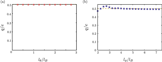
Figure 8: Charge of the edge excitation in a closed system. Charge concentrated close to the edge of the sample as a function of (a) $l_{\theta}$ and (b) $l_{\phi}$. Here $l_{\theta}$ determines the length scale where the angle $\theta(y)$ is varied from $\pi$ to $\theta_{b}$ in the vicinity of the edge and $l_{\phi}$ describes length scale where the angle $\phi(x)$ rotates by $2\pi$. The charge $q$ is computed by integrating the charge density over a single period $l_{\phi}$ along the $x$-direction and over the interval of width $5l_{B}$ from the edge of the sample in $y$-direction. We have chosen $\theta_{b}=\pi/2$ so that the expected charge shown by a dotted line is $q=\nu_{\uparrow}e=e/2$. As expected based on the analytical arguments the value of $q$ is independent on $l_{\theta}$ (as long as the width of the integration interval in $y$-direction is chosen to be larger than the width of the domain wall where the charge is concentrated in the vicinity of the edge), and deviations from the value $e/2$ as a function of $l_{\phi}$ start to occur only when $l_{\phi}\lesssim 4l_{B}$. In the numerics we have chosen the order parameter strength $\Delta_{0}=1$ meV, the width of the sample $W=20l_{B}$, and the space is discretized using a lattice constant $0.25l_{B}$. For (a) we fix $l_{\phi}=5l_{B}$ and for (b) $l_{\theta}=3l_{B}$. The parameters of the BHZ Hamiltonian are same as in Fig. 7.

We have numerically verified the statements based on the analytical arguments given above. For this purpose we have inserted an order parameter term

$$H_{\Delta}=-\Delta_{0}\bigg{[}h_{z}(x,y)\sigma_{z}\tau_{0}+h_{x}(x,y)\sigma_{x}\tau_{x}+h_{y}(x,y)\sigma_{x}\tau_{y}\bigg{]}$$ (54)

to the BHZ Hamiltonian [Eq. (6)]. The charge density associated with the excitation $\delta\rho(\mathbf{r})$ can be numerically computed by calcuting the difference between the charge densities for pseudospin textures $h_{z}(x,y)=\cos[\theta(y)]$, $h_{x}(x,y)=\sin[\theta(y)]\cos[\phi(x)]$, $h_{y}(x,y)=\sin[\theta(y)]\sin[\phi(x)]$, where $\phi(x)=2\pi x/l_{\phi}$ (excited state) and $\phi(x)=0$ (ground state). Here we have introduced a length scale $l_{\phi}$ where the phase $\phi(x)$ rotates over $2\pi$. The charge of an elementary excitation $q$ is obtained by integrating the charge density over a period $l_{\phi}$ in $x$-direction and over the width of the domain wall in $y$-direction. If we choose $l_{\phi}\gg l_{B}$ the charge of the excitation according to our analytic arguments should be $q=\pm\nu_{\uparrow}e$. However, $l_{\phi}$ allows us also to control how fast the pseudospin direction changes in such a way that it influences the system everywhere in the bulk. Therefore, if we choose $l_{\phi}\lesssim l_{B}$ it is possible to excite the higher Landau levels everywhere in the bulk so that topological protection is destroyed, and we can study how this affects the charge of the excitation. Additionally we can illustrate the topological nature of the charge of the pseudospin texture by demonstrating that deformations of the pseudospin texture appearing only close to the edge do not affect the value of $q$. For this purpose we define

$$\theta(y)=\begin{cases}\pi+(\theta_{b}-\pi)y/l_{\theta},&0<y<l_{\theta}\\ \theta_{b},&l_{\theta}<y<W-l_{\theta}\\ \theta_{b}+(\pi-\theta_{b})(y-W+l_{\theta})/l_{\theta},&W-l_{\theta}<y<W\\ \end{cases}$$ (55)

in such a way that $l_{\theta}$ allows to control the length scale where the angle $\theta(y)$ is varied from $\pi$ to $\theta_{b}$ in the vicinity of the edge. Based on our topological arguments the charge $q$ should be independent of $l_{\theta}$. (We assume $W\gg l_{\theta}$.)

The numerical results are shown in Figs. 8. As can be seen from these figures for smooth pseudospin textures the numerical results are in agreement with the analytical expectations. Moreover, $q$ does not depend on $l_{\theta}$ [Fig. 8(a)] in agreement with the topological argument. On the other hand, if we deform the pseudospin texture in such a way that it rotates fast in the bulk by choosing $l_{\phi}\lesssim 4l_{B}$ it is possible to excite the higher Landau levels everywhere in the bulk so that topological protection is destroyed. This results in redistribution of the charges giving rise to deviations of $q$ from the value $\pm\nu_{\uparrow}e$ [Fig. 8(b)].

References

- Sarma and Pinczuk (2008) S. D. Sarma and A. Pinczuk, Perspectives in quantum hall effects: Novel quantum liquids in low-dimensional semiconductor structures (John Wiley & Sons, 2008).
- Jain (2007) J. Jain, Composite Fermions (Cambridge University Press, 2007).
- Read and Green (2000) N. Read and D. Green, Phys. Rev. B 61, 10267 (2000).
- Nayak et al. (2008) C. Nayak, S. H. Simon, A. Stern, M. Freedman, and S. D. Sarma, Rev. Mod. Phys. 80, 1083 (2008).
- Lindner et al. (2012) N. H. Lindner, E. Berg, G. Refael, and A. Stern, Phys. Rev. X 2, 041002 (2012).
- Clarke et al. (2013) D. J. Clarke, J. Alicea, and K. Shtengel, Nature Communications 4, 1348 (2013).
- Mong et al. (2014) R. S. Mong, et al., Phys. Rev. X 4, 011036 (2014).
- Girvin (1999) S. Girvin, The Quantum Hall Effect: Novel Excitations and Broken Symmetries, cond-mat/9907002. IUCM-98-010 (Indiana Univ., Bloomington, IN, 1999).
- Eisenstein and MacDonald (2004) J. Eisenstein and A. MacDonald, Nature 432, 691 (2004).
- Chakraborty and Pietiläinen (1987) T. Chakraborty and P. Pietiläinen, Phys. Rev. Lett. 59, 2784 (1987).
- Fertig (1989) H. Fertig, Phys. Rev. B 40, 1087 (1989).
- Sondhi et al. (1993) S. Sondhi, A. Karlhede, S. Kivelson, and E. Rezayi, Phys. Rev. B 47, 16419 (1993).
- Moon et al. (1995) K. Moon, H. Mori, K. Yang, S. M. Girvin, A. H. MacDonald, L. Zheng, D. Yoshioka, and S.-C. Zhang, Phys. Rev. B 51, 5138 (1995).
- Kane and Mele (2005) C. L. Kane and E. J. Mele, Phys. Rev. Lett. 95, 146802 (2005).
- Bernevig et al. (2006) B. A. Bernevig, T. L. Hughes, and S.-C. Zhang, Science 314, 1757 (2006).
- König et al. (2007) M. König, S. Wiedmann, C. Brüne, A. Roth, H. Buhmann, L. W. Molenkamp, X.-L. Qi, and S.-C. Zhang, Science 318, 766 (2007).
- Liu et al. (2008) C. Liu, T. L. Hughes, X.-L. Qi, K. Wang, and S.-C. Zhang, Phys. Rev. Lett. 100, 236601 (2008).
- Du et al. (2013) L. Du, I. Knez, G. Sullivan, and R.-R. Du, Phys. Rev. Lett. 114, 096802 (2015).
- Spanton et al. (2014) E. M. Spanton, K. C. Nowack, L. Du, G. Sullivan, R.-R. Du, and K. A. Moler, Phys. Rev. Lett. 113, 026804 (2014).
- Scharf et al. (2012) B. Scharf, A. Matos-Abiague, and J. Fabian, Phys. Rev. B 86, 075418 (2012).
- Pikulin et al. (2014) D. I. Pikulin, T. Hyart, S. Mi, J. Tworzydło, M. Wimmer, and C. W. J. Beenakker, Phys. Rev. B 89, 161403 (2014).
- (22) V. Fal’ko and S.V. Iordanskii, Phys. Rev. Lett. 82, 402 (1999).
- (23) H. A. Fertig and L. Brey, Phys. Rev. Lett 97, 116805 (2006).
- Greensite (2011) J. Greensite, An Introduction to the Confinement Problem (Springer, 2011).
- (25) See Supplementary Information for more details.
- Liu and Zhang (2013) C. Liu and S.-C. Zhang, in Topological Insulators, edited by M. Franz and L. W. Molenkamp (Elsevier, Amsterdam, 2013).
- (27) It is known that for sufficiently large interlayer separation the quantum Hall bilayers display an instability towards formation of a charge density wave ground state CoteBreyMacDonald92 . Here we assume that the interlayer separation is small enough that such kind of instability does not occur.
- (28) R. Côté, L. Brey, and A. H. MacDonald, Phys. Rev. B 46, 10239 (1992).
- (29) If is varied with magnetic field the ratio will change within the phase-diagram. Nevertheless, we find that the phase-diagram stays qualitatively similar also in this case.
- Pikulin and Hyart (2014) D. Pikulin and T. Hyart, Phys. Rev. Lett. 112, 176403 (2014).
- (31) D. Zhang, S. Schmult, V. Venkatachalam, W. Dietsche, A. Yacoby, K. von Klitzing, and J. Smet, Phys. Rev. B 87, 205304 (2013).
- (32) F. Nichele et al., Phys. Rev. Lett. 112, 036802 (2014).
- (33) Alternatively, instead of comparing the energies to create elementary excitations in a closed system one could compare the energies needed to create a fixed charge density on the edge. This generalization allows the possibility to consider open systems.
- (34) A. D. K. Finck, J. P. Eisenstein, L. N. Pfeiffer and K. W. West, Phys. Rev. Lett. 106, 236807 (2011).
- (35) X. Huang, W. Dietsche, M. Hauser and K. von Klitzing, Phys. Rev. Lett. 109, 156802 (2012).
- (36) T. Giamarchi, Quantum Physics in One Dimension, (Oxford University Press, 2003).
- (37) C. L. Kane and M. P. A. Fisher, Phys. Rev. B 52, 17393 (1995).
- (38) I. B. Spielman, J. P. Eisenstein, L. N. Pfeiffer and K. W. West, Phys. Rev. Lett. 87, 036803 (2001).
- (39) T. Hyart and B. Rosenow, Phys. Rev. B 83, 155315 (2011).
- (40) G. Murthy, E. Shimshoni, and H. A. Fertig, Phys. Rev. B 90, 241410(R) (2014).
- (41) G. E Volovik, The Universe in a Helium Droplet (Clarendon Press, Oxford, 2003).
- (42) G. E. Volovik, Proc. Nat. Acad. Sci. 97, 2431 (2000).
- (43) Y. Kondo, J. S. Korhonen, M. Krusius, V. V. Dmitriev, E. V. Thuneberg and G. E. Volovik, Phys. Rev. Lett. 68, 3331 (1992).
- (44) K. Yang, K. Moon, L. Belkhir, H. Mori, S. M. Girvin, A. H. MacDonald, L. Zheng, D. Yoshioka, Phys. Rev. B 54, 11644 (1996).
- (45) B. Lake, A. M. Tsvelik, S. Notbohm, D. A. Tennant, T. G. Perring, M. Reehuis, C. Sekar, G. Krabbes and B. Büchner, Nature Physics 6, 50 (2010).
- (46) V. S. Pribiag, A. J.A. Beukman, F. Qu, M. C. Cassidy, C. Charpentier, W. Wegscheider, L. P. Kouwenhoven, Nature Nanotechnology 10, 593 (2015).

References

- Bernevig et al. (2006) B. A. Bernevig, T. L. Hughes, and S.-C. Zhang, Science 314, 1757 (2006).
- Liu et al. (2008) C. Liu, T. L. Hughes, X.-L. Qi, K. Wang, and S.-C. Zhang, Phys. Rev. Lett. 100, 236601 (2008).
- (3)
- (4) L. Du, I. Knez, G. Sullivan, and R.-R. Du, Phys. Rev. Lett. 114, 096802 (2015).
- (5) E. M. Spanton, K. C. Nowack, L. Du, G. Sullivan, R.- R. Du, and K. A. Moler, Phys. Rev. Lett. 113, 026804 (2014).
- (6) P. Michetti, J. C. Budich, E. G. Novik, and P. Recher Phys. Rev. B 85, 125309 (2012).
- Liu and Zhang (2013) C. Liu and S.-C. Zhang, in Topological Insulators, edited by M. Franz and L. W. Molenkamp (Elsevier, Amsterdam, 2013).
- (8)
- (9) K. Moon et al., Phys. Rev. B 51, 5138 (1995).
- (10) I. B. Spielman, L. A. Tracy, J. P. Eisenstein, L. N. Pfeiffer, and K. W. West Phys. Rev. Lett. 94, 076803 (2005).
- (11) P. Giudici, K. Muraki, N. Kumada, Y. Hirayama, and T. Fujisawa Phys. Rev. Lett. 100, 106803 (2008).
- (12) A. D. K. Finck, J. P. Eisenstein, L. N. Pfeiffer, and K. W. West Phys. Rev. Lett. 104, 016801 (2010).
- (13) L. Tiemann, W. Wegscheider, and M. Hauser Phys. Rev. Lett. 114, 176804 (2015).
- (14) F. Qu et al., Phys. Rev. Lett. 115, 036803 (2015).
- (15) L. Du, W. Lou, K. Chang, G. Sullivan, R-R. Du, arXiv:1508.04509.
- (16) F. Nichele et al., Phys. Rev. Lett. 112, 036802 (2014).
- (17) S. Q. Murphy, J. P. Eisenstein, G. S. Boebinger, L. N. Pfeiffer, and K. W. West Phys. Rev. Lett. 72, 728 (1994).
- (18) I. B. Spielman, J. P. Eisenstein, L. N. Pfeiffer, and K. W. West Phys. Rev. Lett. 84, 5808 (2000).
- (19) M. Kellogg, I. B. Spielman, J. P. Eisenstein, L. N. Pfeiffer, and K. W. West Phys. Rev. Lett. 88, 126804 (2002).
- (20) A. R. Champagne, J. P. Eisenstein, L. N. Pfeiffer, and K. W. West Phys. Rev. Lett. 100, 096801 (2008).
- (21) L. Tiemann, Y. Yoon, W. Dietsche, K. von Klitzing, and W. Wegscheider Phys. Rev. B 80, 165120 (2009).
- (22) P. R. Eastham, N. R. Cooper, and D. K. K. Lee, Phys. Rev. B 80, 045302 (2009).
- (23) J. Sun, G. Murthy, H. A. Fertig, and N. Bray-Ali, Phys. Rev. B 81, 195314 (2010).
- (24) A. Stern, S. M. Girvin, A. H. MacDonald, and N. Ma, Phys. Rev. Lett. 86, 1829 (2001).
- (25) H. A. Fertig and G. Murthy, Phys. Rev. Lett. 95, 156802 (2005).
- (26) P. R. Eastham, N. R. Cooper, and D. K. K. Lee, Phys. Rev. Lett. 105, 236805 (2010).
- (27) T. Hyart and B. Rosenow, Phys. Rev. B 83, 155315 (2011).
- (28) T. Hyart and B. Rosenow, Phys. Rev. Lett. 110, 076806 (2013).
- (29) T. Giamarchi, Quantum Physics in One Dimension, (Oxford University Press, 2003).
- (30) D.I. Khomskii and A. Freimuth, Phys. Rev. Lett. 75, 1384 (1995).
- (31) G. Blatter, M. Feigelman, V. Geshkenbein, A. Larkin, and A. van Otterlo, Phys. Rev. Lett. 77, 566 (1996).
- (32) K. Kumagai, K. Nozaki, and Y. Matsuda, Phys. Rev. B 63, 144502 (2001).
- (33) V. D. Natsik, Low Temp. Phys. 31, 915 (2005).
- (34) S. I. Shevchenko, A. S. Rukin, JETP Lett. 90, 42 (2009).
- (35) G.E. Volovik, JETP Lett. 39, 200 (1984).
- (36) A. S. Rukin, S. I. Shevchenko, Low Temp. Phys. 37, 884 (2011),
- (37) I. N. Adamenko and E. K. Nemchenko, Low Temp. Phys. 41, 495 (2015).
- (38) S. Sondhi, A. Karlhede, S. Kivelson, and E. Rezayi, Phys. Rev. B 47, 16419 (1993).
- (39) S. Girvin, The Quantum Hall Effect: Novel Excitations and Broken Symmetries, cond-mat/9907002. IUCM-98- 010 (Indiana Univ., Bloomington, IN, 1999).
- (40) C.-Y. Hou, C. Chamon, and C. Mudry, Phys. Rev. Lett. 98, 186809 (2007).
- (41) S. M. Girvin and A. H. MacDonald, Perspectives in Quantum Hall Effects, edited by S. Das Sarma and A. Pinczuk (Wiley, New York, 1997), Chap. V; arXiv:cond-mat/9505087.