Exploring the proton spin structure
Abstract
Understanding the spin structure of the proton is one of the main challenges in hadronic physics. While the concepts of spin and orbital angular momentum are pretty clear in the context of non-relativistic quantum mechanics, the generalization of these concepts to quantum field theory encounters serious difficulties. It is however possible to define meaningful decompositions of the proton spin that are (in principle) measurable. We propose a summary of the present situation including recent developments and prospects of future developments.
1 Introduction
Understanding how the proton spin arises from the spin and orbital motion of its constituents is one the most challenging key questions in hadronic physics. Hadrons are very peculiar physical systems as their constituents are highly relativistic and confined. One has therefore to use cunning in order to unravel their internal structure.
While it is clear that a proton at rest has total angular momentum , the decomposition of the latter in terms of spin and orbital contributions associated with quarks and gluons is not unique, creating some confusion and raising serious controversies among physicists. Most of the discussions focused on determining which one of the proposed decompositions has to be considered as the “physical” or fundamental one. Now that the dust has settled, it turns out that the angular momentum decomposition is intrinsically ambiguous because of Lorentz and gauge symmetry. However, this does not imply that the question of the angular momentum decomposition does not make sense at all, but rather emphasizes the fact that the description of a physical phenomenon does not need to be unique. What is considered as the “physical” or fundamental description usually turns out to be the simplest or most convenient description at hand.
While measurable quantities are necessarily gauge invariant, it has recently been recognized that they need not be local or manifestly Lorentz covariant. Departing from locality or manifest Lorentz covariance leads to ambiguities as there exists in principle infinitely many ways to do so. What saves the day is that it is the way the physical system is probed, i.e. the experimental configuration, which determines the natural or sensible departure from locality or manifest Lorentz covariance. For example, the internal structure of the proton is essentially probed in high-energy experiments which provide us with a natural preferred direction breaking manifest Lorentz covariance. This preferred direction can then be used to define the natural angular momentum decomposition.
One of the crucial questions now is to identify the experimental observables from which the orbital angular momentum (OAM) can be extracted. Many different relations and sum rules have been proposed in the last two decades, creating some sort of confusion. One of the remaining tasks consists in clarifying the validity and scope of these relations and sum rules.
In this contribution, we summarize the present situation and mention some recent developments. In section 2, we briefly discuss the two families of proton spin decompositions. In section 3, we collect various spin sum rules and relations. In section 4, we introduce the notion of quark spin-orbit correlation and show how it is related to measurable parton distributions. Finally, we collect our conclusions in section 5. For the interested reader, more detailed discussions can be found in the recent reviews Leader:2013jra ; Wakamatsu:2014zza .
2 Kinetic and canonical spin decompositions
There are essentially two types of decompositions of the proton spin operator: kinetic (also known as mechanical) and canonical. These two types differ by how the OAM operator is split into the quark () and gluon () contributions
| (1) | ||||
where
| (2) | ||||||
The gauge field has been decomposed into two parts where is a pure-gauge potential. The pure-gauge covariant derivatives are then given by and . A nice physical interpretation of the difference , known as the potential OAM, has been proposed in Ref. Burkardt:2012sd .
The complete gauge-invariant kinetic and canonical decompositions (1) are known in the literature as the Wakamatsu Wakamatsu:2010qj ; Wakamatsu:2010cb and Chen et al. Chen:2008ag ; Chen:2009mr decompositions, respectively. The Chen et al. decompositon can be seen as a gauge-invariant version (or extension) of the Jaffe-Manohar decomposition Jaffe:1989jz . These complete gauge-invariant decompositions seem to contradict textbook claims about the impossibility of separating in a gauge-invariant way the gluon angular momentum into spin and OAM contributions. This impossibility is circumvented by introducing the non-local fields and Lorce:2012rr ; Lorce:2012ce , where the pure-gauge field plays the role of a background field Lorce:2013gxa ; Lorce:2013bja . Background dependence then implies that the decomposition comes with a new freedom
| (3) |
referred to as the Stueckelberg symmetry Lorce:2012rr ; Stoilov:2010pv , making the decompositions ambiguous as a priori any pure-gauge field can be used. This issue is however solved by noting that the actual experimental conditions determine the form of the background field to be used Lorce:2012rr ; Wakamatsu:2014toa .
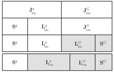
Incomplete kinetic decompositions avoid the uniqueness issue from the beginning. In the Ji decomposition Ji:1996ek , the gluon spin and OAM contributions are combined to form the gluon total angular momentum
| (4) |
which is local and therefore free from the Stueckelberg ambiguity. In the Belinfante decomposition, one further combines the quark spin and OAM contributions into the quark total angular momentum
| (5) |
so that one can write with where is the symmetric kinetic (or Belinfante-Rosenfeld) energy-momentum tensor. See Fig. 1 for a summary of the decompositions.
3 Spin sum rules and relations
Using the Belinfante-Rosenfeld version of the energy-momentum tensor, Ji obtained the remarkable result that the quark/gluon total kinetic angular momentum can be expressed in terms of twist-2 generalized parton distributions (GPDs) Ji:1996ek
| (6) |
This relation holds for the longitudinal component and does not depend on the magnitude of the proton momentum Ji:1997pf ; Leader:2011cr ; Leader:2012md . By rotational symmetry, it is also valid for the transverse component, but only in the proton rest frame. Considering the transverse component of the Pauli-Lubanski vector does not prevent frame dependence of the separate quark and gluon contributions Leader:2012ar ; Leader:2013jra ; Hatta:2012jm ; Harindranath:2013goa .
Subtracting from Eq. (6) the longitudinal quark spin contribution, which is given by the isoscalar axial-vector form factor (FF) in the scheme
| (7) |
one obtains the following expression for the longitudinal quark kinetic OAM
| (8) |
The same quantitie can also be expressed in terms of a twist-3 GPD Penttinen:2000dg ; Kiptily:2002nx ; Hatta:2012cs ; Lorce:2015lna
| (9) |
which appears in the longitudinal target spin asymmetry of deeply virtual Compton scattering Courtoy:2013oaa .
The most intuitive expression for OAM is as a phase-space integral Lorce:2011kd ; Lorce:2011ni
| (10) |
where the relativistic phase-space or Wigner distribution can be interpreted as giving the (quasi-)probability for finding an unpolarized quark/gluon with momentum at the transverse position inside a longitudinally polarized proton. In this semi-classical interpretation, the Euclidean subgroup of the light-front formalism plays a crucial role in providing a well-defined transverse center of the proton Soper:1976jc ; Burkardt:2000za ; Burkardt:2005hp . These phase-space distributions are related by Fourier transform to the so-called generalized transverse-momentum dependent distributions (GTMDs) Meissner:2009ww ; Lorce:2011dv ; Lorce:2013pza , leading to the simple relation Lorce:2011kd ; Hatta:2011ku ; Kanazawa:2014nha
| (11) |
The type of OAM is determined by the shape of the Wilson line , namely and Burkardt:2012sd ; Lorce:2012ce ; Ji:2012sj . Unfortunately, it is not known so far how to extract GTMDs from actual experiments, except perhaps at small Meissner:2009ww . Interestingly, they are however in principle calculable on the lattice Ji:2013dva .
In the context of quark models, it has also been suggested that the quark canonical OAM could be related to a transverse-momentum dependent distribution (TMD)
| (12) |
but this relation is not valid in general in QCD Lorce:2011kn just like other relations among the TMDs Lorce:2011zta . In Table 3, the various expressions (8), (11) and (12) for the quark OAM are compared in two light-front quark models: the light-front constituent quark model (LFCQM) Boffi:2002yy ; Boffi:2003yj ; Pasquini:2005dk ; Pasquini:2006iv ; Pasquini:2008ax and the light-front chiral quark-soliton model (LFQSM) Lorce:2006nq ; Lorce:2007as ; Lorce:2007fa . While all the expressions agree for the total OAM, as they should, they differ in the flavor decomposition.
| Model | LFCQM | LFQSM | |||||
|---|---|---|---|---|---|---|---|
| Total | Total | ||||||
| \svhline | Eq. (8) | ||||||
| Eq. (11) | |||||||
| Eq. (12) | |||||||
4 Spin-orbit correlation
What is referred to as the quark spin/OAM contribution to the proton spin corresponds more precisely to the correlation between the quark spin/OAM and the proton spin. There exists another interesting independent correlation characterizing the proton spin structure, although it does not appear in the proton spin decomposition, namely the correlation between the quark spin and the quark OAM. Like the OAM operators, one can define a kinetic and a canonical version of this spin-orbit correlation Lorce:2011kd ; Lorce:2014mxa
| (13) | ||||
Like the average kinetic OAM contribution to the proton spin, the average quark longitudinal spin-orbit correlation can be expressed in terms of twist-2 and twist-3 GPDs Lorce:2014mxa
| (14) | ||||
Remarkably, this shows that not only the first moment but also the second moment of the quark helicity distribution has physical interest.
The quark spin-orbit correlation can naturally also be expressed as a phase-space integral Lorce:2011kd ; Lorce:2014mxa
| (15) |
where the relativistic phase-space distribution can be interpreted as giving the difference between the (quasi-)probabilistic distributions of quarks with polarization parallel and antiparallel to the longitudinal direction. In terms of the GTMDs, this relation reads Lorce:2011kd ; Kanazawa:2014nha ; Lorce:2014mxa
| (16) |
Once again, the shape of the Wilson line determines the type of spin-orbit correlation, namely and Lorce:2014mxa .
Because of the valence number constraints and and the small mass ratio , the essential non-perturbative input we need is the second moment of the quark helicity distribution
| (17) |
Contrary to the lowest moment , this second moment cannot simply be extracted from deep-inelastic scattering (DIS) polarized data. However, by combining inclusive and semi-inclusive DIS, separate quark and antiquark contributions can be extracted Leader:2010rb . They can also be computed on the lattice Bratt:2010jn . In Table 4, the first two moments of the quark helicity distributions computed within the naive quark model (NQM), the LFCQM and the LFQSM are compared with the values obtained from inclusive and semi-inclusive DIS data Leader:2010rb and from lattice calculations Bratt:2010jn .
| Model | |||||
| \svhline NQM | |||||
| LFCQM | |||||
| LFQSM | |||||
| \svhline LSS Leader:2010rb | |||||
| Lattice Bratt:2010jn | |||||
From these estimates, one obtains a negative kinetic quark spin-orbit correlation for both quark flavors, and , meaning that in average the quark spin and kinetic OAM are expected to be antiparallel. On the contrary, the canonical version of the quark spin-orbit correlation appears to be positive in the models Lorce:2011kd , showing the importance of the quark-gluon interaction.
5 Conclusion
There are essentially two types of proton spin decompositions: the kinetic one and the canonical one. It has recently been recognized that both are interesting and in principle measurable. The crucial missing piece in the proton spin decomposition is the contribution coming from the quark and gluon orbital angular momentum. Several relations and sum rules have been proposed in the literature, but few proved to be of practical significance. The current most promising approaches are based on the extraction of generalized parton distributions at twist 2 and 3 from experiments, and the direct calculation of orbital angular momentum on the lattice.
Another important aspect of the proton spin structure is the spin-orbit correlation which escaped attention until recently because it does not contribute to the proton spin decomposition. Like the orbital angular momentum, there are two types of spin-orbit correlations, and both are in principle measurable. This piece of information is of crucial importance if one aims at obtaining a complete description of the proton spin structure.
Acknowledgements.
I benefited a lot from many discussions and collaborations with E. Leader, B. Pasquini and M. Wakamatsu. This work was supported by the Belgian Fund F.R.S.-FNRS via the contract of Chargé de Recherches.References
- (1) S. Boffi, B. Pasquini, and M. Traini, Nucl. Phys. B 649, 243 (2003).
- (2) S. Boffi, B. Pasquini, and M. Traini, Nucl. Phys. B 680, 147 (2004).
- (3) J. D. Bratt et al. [LHPC Collaboration], Phys. Rev. D 82, 094502 (2010).
- (4) M. Burkardt, Phys. Rev. D 62, 071503 (2000) [Erratum-ibid. D 66, 119903 (2002)].
- (5) M. Burkardt, Phys. Rev. D 72, 094020 (2005).
- (6) M. Burkardt, Phys. Rev. D 88, no. 1, 014014 (2013).
- (7) X. -S. Chen, X. -F. Lu, W. -M. Sun, F. Wang and T. Goldman, Phys. Rev. Lett. 100, 232002 (2008).
- (8) X. -S. Chen, W. -M. Sun, X. -F. Lu, F. Wang and T. Goldman, Phys. Rev. Lett. 103, 062001 (2009).
- (9) A. Courtoy, G. R. Goldstein, J. O. G. Hernandez, S. Liuti and A. Rajan, Phys. Lett. B 731, 141 (2014).
- (10) A. Harindranath, R. Kundu and A. Mukherjee, Phys. Lett. B 728, 63 (2014).
- (11) Y. Hatta, Phys. Lett. B 708, 186 (2012).
- (12) Y. Hatta and S. Yoshida, JHEP 1210, 080 (2012).
- (13) Y. Hatta, K. Tanaka and S. Yoshida, JHEP 1302, 003 (2013).
- (14) R. L. Jaffe and A. Manohar, Nucl. Phys. B 337, 509 (1990).
- (15) X. -D. Ji, Phys. Rev. Lett. 78, 610 (1997).
- (16) X. D. Ji, Phys. Rev. D 58, 056003 (1998).
- (17) X. Ji, Phys. Rev. Lett. 110, 262002 (2013).
- (18) X. Ji, X. Xiong and F. Yuan, Phys. Rev. Lett. 109, 152005 (2012).
- (19) K. Kanazawa, C. Lorcé, A. Metz, B. Pasquini and M. Schlegel, Phys. Rev. D 90, 014028 (2014).
- (20) D. V. Kiptily and M. V. Polyakov, Eur. Phys. J. C 37, 105 (2004).
- (21) E. Leader, Phys. Rev. D 85, 051501 (2012).
- (22) E. Leader, Phys. Lett. B 720, 120 (2013).
- (23) E. Leader and C. Lorcé, Phys. Rev. Lett. 111, 039101 (2013).
- (24) E. Leader and C. Lorcé, Phys. Rept. 541, 163 (2014).
- (25) E. Leader, A. V. Sidorov and D. B. Stamenov, Phys. Rev. D 82, 114018 (2010).
- (26) C. Lorcé, Phys. Rev. D 74, 054019 (2006).
- (27) C. Lorcé, Phys. Rev. D 78, 034001 (2008).
- (28) C. Lorcé, Phys. Rev. D 79, 074027 (2009).
- (29) C. Lorcé, Phys. Rev. D 87, 034031 (2013).
- (30) C. Lorcé, Phys. Lett. B 719, 185 (2013).
- (31) C. Lorcé, Phys. Rev. D 88, 044037 (2013).
- (32) C. Lorcé, Nucl. Phys. A 925, 1 (2014).
- (33) C. Lorcé, Phys. Lett. B 735, 344 (2014).
- (34) C. Lorcé, arXiv:1502.06656 [hep-ph].
- (35) C. Lorcé and B. Pasquini, Phys. Rev. D 84, 014015 (2011).
- (36) C. Lorcé and B. Pasquini, Phys. Rev. D 84, 034039 (2011).
- (37) C. Lorcé and B. Pasquini, Phys. Lett. B 710, 486 (2012).
- (38) C. Lorcé and B. Pasquini, JHEP 1309, 138 (2013).
- (39) C. Lorcé, B. Pasquini and M. Vanderhaeghen, JHEP 1105, 041 (2011).
- (40) C. Lorcé, B. Pasquini, X. Xiong and F. Yuan, Phys. Rev. D 85, 114006 (2012).
- (41) S. Meissner, A. Metz and M. Schlegel, JHEP 0908, 056 (2009).
- (42) B. Pasquini, M. Pincetti and S. Boffi, Phys. Rev. D 72, 094029 (2005).
- (43) B. Pasquini, M. Pincetti and S. Boffi, Phys. Rev. D 76, 034020 (2007).
- (44) B. Pasquini, S. Cazzaniga, and S. Boffi, Phys. Rev. D 78, 034025 (2008).
- (45) M. Penttinen, M. V. Polyakov, A. G. Shuvaev and M. Strikman, Phys. Lett. B 491, 96 (2000).
- (46) D. E. Soper, Phys. Rev. D 15, 1141 (1977).
- (47) M. N. Stoilov, arXiv:1011.5617 [hep-th].
- (48) M. Wakamatsu, Phys. Rev. D 81, 114010 (2010).
- (49) M. Wakamatsu, Phys. Rev. D 83, 014012 (2011).
- (50) M. Wakamatsu, Int. J. Mod. Phys. A 29, 1430012 (2014).
- (51) M. Wakamatsu, arXiv:1409.4474 [hep-ph].