Exploiting Local Features from Deep Networks for Image Retrieval
Abstract
Deep convolutional neural networks have been successfully applied to image classification tasks. When these same networks have been applied to image retrieval, the assumption has been made that the last layers would give the best performance, as they do in classification. We show that for instance-level image retrieval, lower layers often perform better than the last layers in convolutional neural networks. We present an approach for extracting convolutional features from different layers of the networks, and adopt VLAD encoding to encode features into a single vector for each image. We investigate the effect of different layers and scales of input images on the performance of convolutional features using the recent deep networks OxfordNet and GoogLeNet. Experiments demonstrate that intermediate layers or higher layers with finer scales produce better results for image retrieval, compared to the last layer. When using compressed 128-D VLAD descriptors, our method obtains state-of-the-art results and outperforms other VLAD and CNN based approaches on two out of three test datasets. Our work provides guidance for transferring deep networks trained on image classification to image retrieval tasks.
1 Introduction
Image retrieval has been an active research topic for decades. Most existing approaches adopt low-level visual features, i.e., SIFT descriptors, and encode them using bag-of-words (BoW), vector locally aggregated descriptors (VLAD) or Fisher vectors (FV) and their variants. Since SIFT descriptors capture local characteristics of objects, such as edges and corners, they are particularly suitable for matching local patterns of objects for instance-level image retrieval.
Recently, convolutional neural networks (CNNs) demonstrated excellent performance on image classification problems such as PASCAL VOC and ImageNet Large Scale Visual Recognition Challenge (ILSVRC) [17, 31, 29, 34]. By training multiple layers of convolutional filters, CNNs are capable to automatically learn complex features for object recognition and achieve superior performance compared to hand-crafted features. A few works have suggested that CNNs trained for image classification tasks can be adopted to extract generic features for other visual recognition tasks [6, 25, 19]. Although several approaches have applied CNNs to extract generic features for image retrieval tasks and obtained promising results, a few questions still remain unaddressed. First, by default CNNs are trained for classification tasks, where features from the final layer (or higher layers) are usually used for decision because they capture more semantic features for category-level classification. However, local characteristics of objects at the instance level are not well preserved at higher levels. Therefore, it is questionable whether it is best to directly extract features from the final layer or higher layers for instance-level image retrieval, where different objects from the same category need to be separated. Second, most existing work assumes the size of a test image is the same as that of the training images. However, different scales of input images may affect the behavior of convolutional layers as images pass through the network. Only a few recent works attempt to investigate such effects on the performance of CNNs for image retrieval [8, 26].
In view of the power of low-level features (i.e., SIFT) in preserving the local patterns of instances, and the success of CNN features in abstracting categorical information, we process CNN activations from lower to higher layers to construct a new feature for image retrieval by VLAD, although other encoding schemes can be readily applied. Recent deep networks OxfordNet and GoogLeNet pre-trained on ImageNet database are used for evaluation. We find that features from lower layers capture more local patterns of objects, and thus perform better than features from higher layers for instance-level image retrieval, which indicates that it is not the best choice to directly apply the final layer or higher layers that are designed for classification tasks to instance-level image retrieval. In addition, we conduct further experiments by changing the scale of input images and using the same feature extraction and encoding methods. It is surprising that the behavior of filters in each layer changes significantly with respect to the scale of input images. With input images of higher resolution, even the filters at higher layers effectively capture local characteristics of images as well, apart from semantic concepts of objects, thus producing better features and subsequent better retrieval results.
The contributions of this work are three-fold. First, we design and conduct systematic and thorough experiments to investigate the performance of features from different layers and different scales of input test images in instance-level image retrieval. Second, we introduce using VLAD encoding of local convolutional features from CNNs for image retrieval. The new convolutional feature mimics the ability of SIFT descriptors to preserve local characteristics of objects, in addition to the well-known power of CNNs of capturing category-level information. Our framework, based on the new features, outperforms other VLAD and CNN based approaches even with a relatively low-dimensional representation. Finally, we provide insights as to why lower layers should be used for instance-level image retrieval rather than higher layers, while higher layers may achieve better performance for high resolution input images.
2 Related Work
Traditional image retrieval approaches rely on hand-crafted features like SIFT descriptors, which are usually encoded into bag-of-words (BoW) histograms [30]. To increase the discriminative ability of SIFT descriptors, RootSIFT [1] was proposed to address the burstiness problem by using the Hellinger kernel on the original SIFT descriptors. Jégou et al. [11] proposed the vector locally aggregated descriptor (VLAD) to obtain a compact representation as a replacement for BoW histograms, which achieves good results while requiring less storage. PCA and whitening [9], signed square root (SSR) on VLAD vectors [11] and intra-normalization [2] are later applied to the original VLAD descriptors to reduce noise and further boost performance. Multi-VLAD [2] is based on constructing and matching VLAD features of multiple levels from an image to improve localization accuracy. Other global features such as GIST descriptors and Fisher Vector (FV) [21] have also been evaluated for large-scale image retrieval. Some approaches rely on semantic concepts or attributes to capture mid-level image information [7, 28, 24], where attributes are binary values indicating the presence of semantic characteristics. Relative attributes have been widely applied to refine search results. In [16], a set of ranking functions are learned offline to predict the strength of attributes, which are then updated by relative attribute feedback to rerank relevant images from the query stage. Implicit feedback [20] to learn ranking functions using implied user feedback cues and pivot attributes selection [15] to reduce the system’s uncertainty have also been proposed to improve reranking performance. [14] learns a generic prediction function and adapts it into a user-specific function using user-labeled samples for personalized image search.
CNNs have led to major improvements in image classification [6, 25, 19]. As a universal image representation, CNN features can be applied to other recognition tasks and perform well [19, 6, 34]. Razavian et al. [25] first investigated the use of CNN features, i.e., OverFeat [27], for various computer vision tasks, including image retrieval. However, the performance of CNN feature extracted from the final layer lags behind that of simple SIFT-based methods with BoW and VLAD encoding. Only by additionally incorporating spatial information do they achieve comparable results. In [4], CNN features learned from natural images with various augmentation and pooling schemes are applied to painting retrieval and achieve good results. Gong et al. [8] introduce Multi-scale Orderless Pooling (MOP) to aggregate CNN activations from higher layers with VLAD, where these activations are extracted by a sliding window with multiple scales. Experiments on an image retrieval dataset have shown promising results, but choosing which scales and layers to use remains unclear. In [3], a CNN model is retrained on a separate landmark database that is similar to the images at query time. Not surprisingly, features extracted from the retrained CNN model obtain very good performance. Unfortunately, collecting training samples and retraining the entire CNN model requires significant amounts of human and computing resources, making the application of this approach rather limited. [32] conducted a comprehensive study on applying CNN features to real-world image retrieval with model retraining and similarity learning. Encouraging experimental results show that CNN features are effective in bridging the semantic gap between low-level visual features and high-level concepts. Recently, [26] conducted extensive experiments on different instance retrieval dataset and obtained excellent results by using spatial search with CNN features. Our work is inspired by [8] which also employs VLAD on CNN activations on multi-scale setting, but fundamentally different from [8]. They utilize higher layers and multi-scale sliding window to extract CNN features from multiple patches independently, so the network has to be applied multiple times. In contrast, we apply the network only once to the input image, and extract features at each location of the convolutional feature map in each layer. We also explicitly verify the effectiveness of intermediate layers for image retrieval and provide additional analysis on the effect of scale.
[33] introduces latent concept descriptors for video event detection by extracting and encoding features using VLAD at the last convolutional layer with spatial pooling. In contrast, we extend the use of convolutional features to lower layers without additional pooling to preserve local information. We also focus on evaluating performance of different convolutional layers for instance-level image retrieval.
3 Approach
We describe our approach of extracting and encoding CNN features for image retrieval in this section. We start by introducing the deep neural networks used in our framework, and then describe the method for extracting features. To encode features for efficient retrieval, we adopt VLAD to compress the CNN features into a compact representations.
3.1 Convolutional neural network
Our approach is applicable to various convolutional neural network architectures. We experiment with two variants of recent deep neural networks: OxfordNet [29] and GoogLeNet [31], which ranked top two in ILSVRC 2014. The networks are pre-trained on ImageNet by Caffe implementation [13] and publicly available on the Caffe model zoo. We adopt the 16 layers OxfordNet trained by [29] as it gives similar performance to the 19 layer version. The network consists of stacked convolutional layers and pooling layers, followed by two fully connected layers and takes images of pixels as input. We also use a 22-layer deep convolutional network GoogLeNet [31], which gives state-of-the-art results in ImageNet classification tasks. The GoogLeNet takes images of pixels as input that is then passed through multiple convolutional layers and stacking “inception” modules. Each inception module is regarded as a convolutional layer containing , and convolutions, which are concatenated with an additional max pooling, with convolutional layers in between for dimensionality reduction. There are totally 9 inception modules sequentially connected, followed by an average pooling and a softmax at the end. Unlike OxfordNet, fully connected layers are eliminated which simplifies our experiments, so that we can focus on the convolutional feature maps. Finally, the networks are trained by average-pooled activation followed by softmax. The fully convolutional network GoogLeNet simplifies the extension to applying the network to multiple scales of images, and lets us encode the local convolutional features in the same way for all layers, which allows fair comparisons among layers. Table 1 shows the output size of intermediate layers in OxfordNet and GoogLeNet. Since it is time consuming to evaluate the lower layers which have large feature maps, some lower layers are omitted in our evaluation.
3.2 Extracting convolutional features
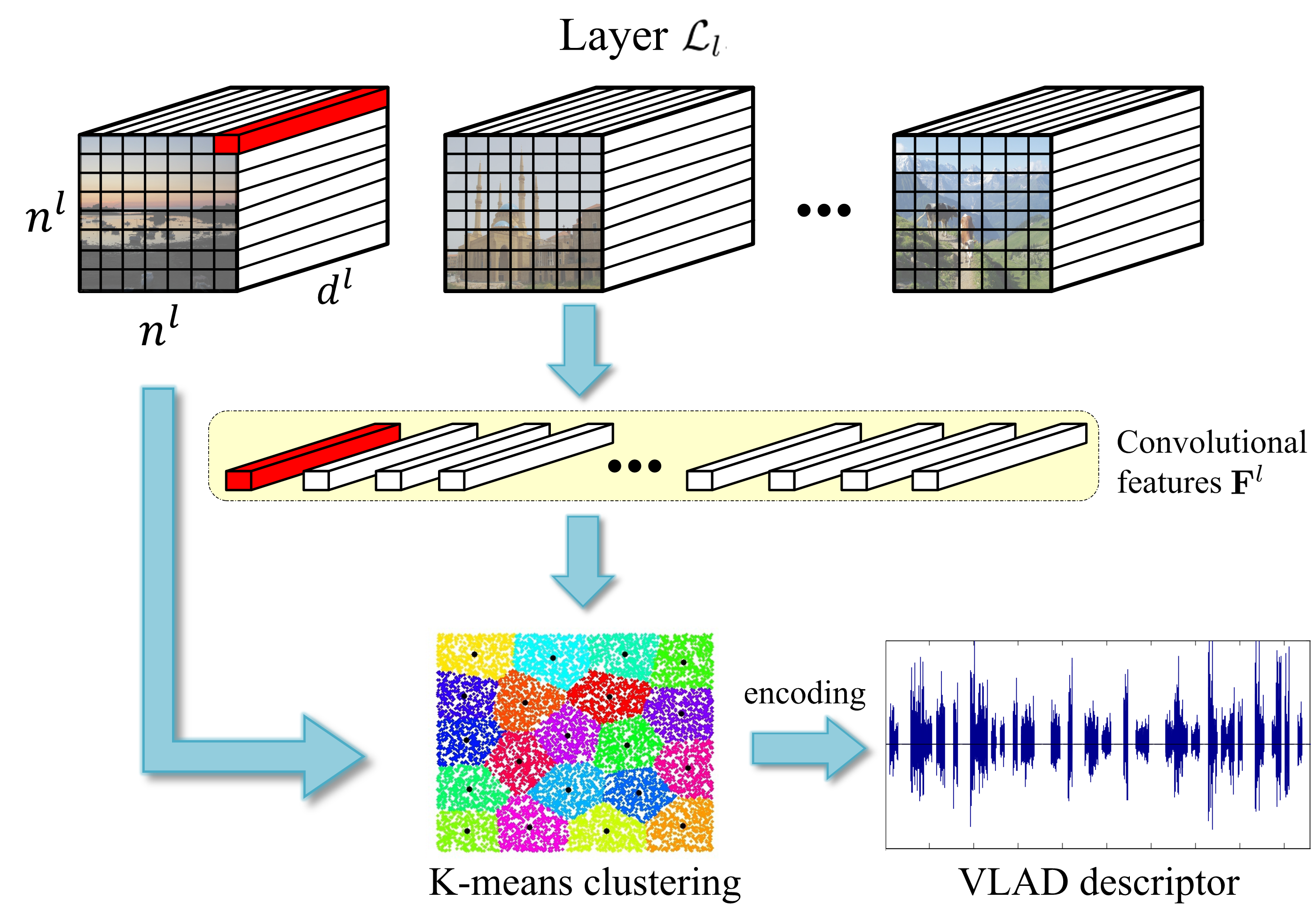
Given a pre-trained network (OxfordNet or GoogLeNet) with layers, an input image is first warped into an square to fit the size of training images, and then is passed through the network in a forward pass. In the -th convolutional layer , after applying the filters to the input image , we obtain an feature map , where is the number of filters with respect to . For notational simplicity, we denote . Similar to the strategy in [33], at each location and , in the feature map , we obtain a -dimensional vector containing activations of all filters, which is considered as our feature vector. In this way, we obtain local feature vectors for each input image at the convolutional layer , denoted as . While [33] only extracts features from the last convolutional layer, we extend the feature extraction approach to all convolutional layers. By processing the input image throughout the network, we finally obtain a set of feature vectors for each layer, . The feature extraction procedure is illustrated in Figure 1111The k-means clustering figure is from http://www.vlfeat.org/overview/kmeans.html.
3.3 VLAD encoding
Unlike image classification, which is trained with many labeled data for every category, in instance retrieval generally there is no training data available. Therefore, a pre-trained network is likely to fail to produce good holistic representations that are invariant to translation or viewpoint changes while preserving instance level information. In contrast, local features, which focus on smaller parts of images, are easier to represent and generalize to other object categories while capturing invariance.
Since each image contains a set of low-dimensional feature vectors, which has similar structure as dense SIFT, we propose to encode these feature vectors into a single feature vector using standard VLAD encoding. The VLAD encoding is effective for encoding local features into a single descriptor while achieving a favorable trade-off between retrieval accuracy and memory footprint. An overview of our system is illustrated in Figure 1.
| Layer (low high) | Output size () |
|---|---|
| pool1-norm1 | |
| conv2-norm2 | |
| Inception 3a | |
| Inception 3b | |
| Inception 4a | |
| Inception 4b | |
| Inception 4c | |
| Inception 4d | |
| Inception 4e | |
| Inception 5a | |
| Inception 5b |
| Layer (low high) | Output size () |
|---|---|
| conv2_1 | |
| conv2_2 | |
| conv2_3 | |
| conv3_1 | |
| conv3_2 | |
| conv3_3 | |
| conv4_1 | |
| conv4_2 | |
| conv4_3 | |
| conv5_1 | |
| conv5_2 | |
| conv5_3 |
VLAD encoding is similar to constructing BoW histograms. Given a collection of L2-normalized convolutional features from layer , we perform k-means clustering to obtain a vocabulary of visual words, where is relatively small ( in our experiments following [8]), so the vocabulary is coarse. For each image, a convolutional feature from layer is assigned to its nearest visual word . For the visual word , the vector difference between and the feature (residual), , is recorded and accumulated for all features assigned to . The VLAD encoding converts the set of convolutional features of an image, , from layer to a single -dimensional vector , describing the distribution of feature vectors regarding the visual words. Formally, a VLAD descriptor of an image regarding layer is represented as
| (1) |
Here is the accumulated residual between the visual word and all convolutional features that are assigned to . The VLAD descriptors are normalized by intra-normalization which has been shown to give superior results than signed square root (SSR) normalization [2]. Since the dimensionality of the original VLAD descriptor is very high, making direct comparison expensive, we further apply PCA to reduce the dimensionality of VLAD descriptors to improve retrieval efficiency and then whitening to increase its robustness against noise.
3.4 Image Retrieval
For all database images and a query image, we extract convolutional features and encode them into VLAD descriptors. Image retrieval is done by calculating the L2 distance between the VLAD descriptors of the query image and database images. We use PCA to compress the original VLAD descriptors to relatively low-dimensional vectors (128-D), so that the computation of L2 distance can be done efficiently. We will show in the experiments that the compressed 128-D VLAD vectors achieve excellent results with little loss of performance.
4 Experiments
We perform experiments on 3 instance-level image retrieval datasets: Holidays [10], Oxford [22] and Paris [23]. The Holidays dataset includes 1491 images of personal holiday photos from 500 categories, where the first image in each category is used as the query. The Oxford and Paris datasets consist of 5062 images and 6412 images of famous landmarks in Oxford and Paris, respectively. Both datasets have 55 queries with specified rectangular region of interest enclosing the instance to be retrieved, where each landmark has multiple query images. To simplify the experiments, the rectangular regions are ignored and full images are used for retrieval in this work. Following the standard evaluation protocol, we use mean average precision (mAP) to evaluate the performance of our approach.
4.1 Comparison of layers
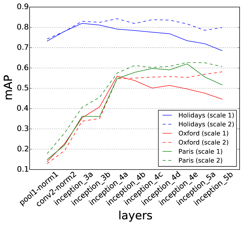
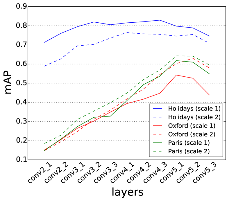
We first study the performance of convolutional features from different layers. We use VLAD to encode convolutional features from each layer and evaluate the mAP with respect to the corresponding layer. Figure 2 shows the performance for both OxfordNet and GoogLeNet. There is a clear trend in the results of both networks on the first scale (solid lines in the figure). The mAP first increases as we go deeper into the network because the convolutional features achieve more invariance, until reaching a peak. However, the performance at higher layers gradually drops since the features are becoming too generalized and less discriminative for instance-level retrieval. The best performing layers of GoogLeNet on the Holidays, Oxford and Paris datasets are Inception 3a, Inception 4a, and Inception 4e respectively. On the Holidays dataset, the performance of intermediate layers is much better than that of the last layer (82.0% vs 68.5%). In contrast, the best performing layers on the Oxford and Paris datasets are from middle upper layers. Nevertheless, similar trends can still be clearly seen on these two datasets that the intermediate layers perform better than the last layer. We then conduct similar experiment with the 16 layers OxfordNet. Although OxfordNet is less deeper than GoogLeNet, we still see this trend. On the Oxford and Paris datasets, the best performing layer is not the last layer, but the intermediate convolutional layers conv5_1, showing that increasing generalization at higher layers is not always useful in instance retrieval. This verifies that across different network architectures and datasets, intermediate layers perform the best and should be used for instance-level retrieval.
When convolutional networks grow deeper, which gives an increasing number of choice for layers to transfer, it becomes more important to examine the layers used for image retrieval, since the layers perform very differently in deep networks. Unlike recent work, which suggests only using the last two fully connected layers [25, 8, 3], or the last convolutional layers [26], our experiments show that higher layers are not always optimal depending on the tasks considered, especially for the very deep networks recently proposed. For instance-level image retrieval, which is very different from classification tasks, lower layers usually perform better than higher layers as features from lower layers preserve more local and instance-level characteristics of objects. We envisage this trend will become more pronounced when networks become deeper in the future.
4.2 Scales
Applying a network at multiple scales gives significant improvement over its original scale as shown in previous work [8, 25]. In view of this, apart from using the original size of input images (scale 1), we enlarge the size of the input image to (scale 2) to generate 4 times larger feature maps at each layer, and conduct similar experiments. We evaluate the difference in performance using features extracted from scale 1 and scale 2.
Figure 2 shows the performance of different layers at both scales. In general, features from the finer scale, which are obtained from higher resolution images, give better performance than the original scale except OxfordNet on the Holidays dataset. Interestingly, the relative performance among layers at the higher scale are quite different from the original scale from GoogLeNet. On the Holidays dataset, the performance at scale 2 first increases and then decreases as we go up to higher layers. The trend is similar to scale 1 although the performance difference between layers at scale 2 is smaller. On the Oxford and Paris datasets, we obtain better results using features from higher layers than those from lower layers on the finer scale (scale 2). It is surprising that the networks perform better with larger input images, although by default they should take images of pixels that they are trained on as the input [26]. An intuitive explanation for the good performance of the last layer at scale 2 is that the original filters focus more on local details of enlarged images since the size of the filters remains unchanged. Therefore, the convolutional features extracted from the higher layers at a finer scale actually focuses on smaller parts of the images, thus preserving mid-level details of objects to some extent instead of global categorical and abstract information as in the original scale. Our experiments suggest that higher resolution images are preferable even if the network was trained at a coarser level. In contrast, different layers in OxfordNet, which was trained in a multi-scale setting, behave similarly for both scales.
| Original images | Inception 4a | Inception 5b | Inception 5b (scale 2) | |
|---|---|---|---|---|
 |
 |
 |
 |
1-NN |
 |
 |
 |
5-NN | |
 |
 |
 |
 |
1-NN |
 |
 |
 |
5-NN |
4.3 Feature visualization
To further understand the features of different layers and scales, we produce visualizations of GoogLeNet features based on the Holidays dataset.
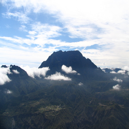
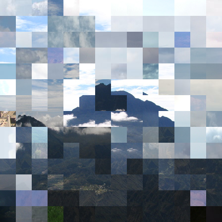
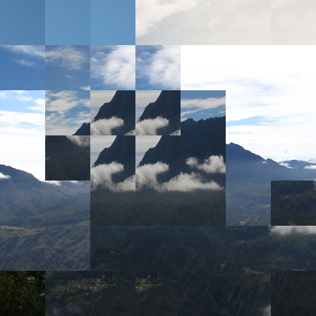
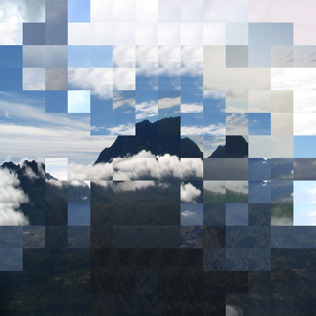
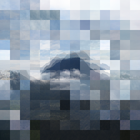
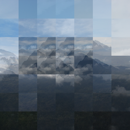
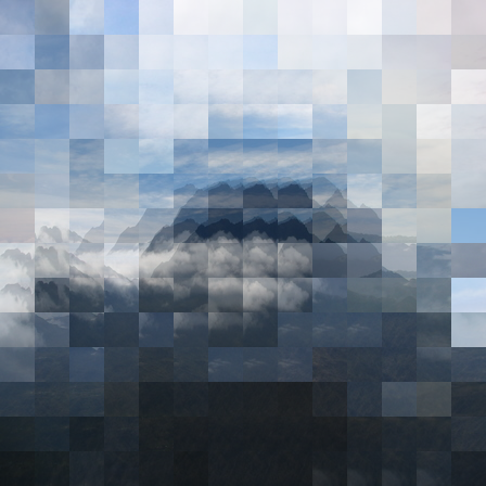
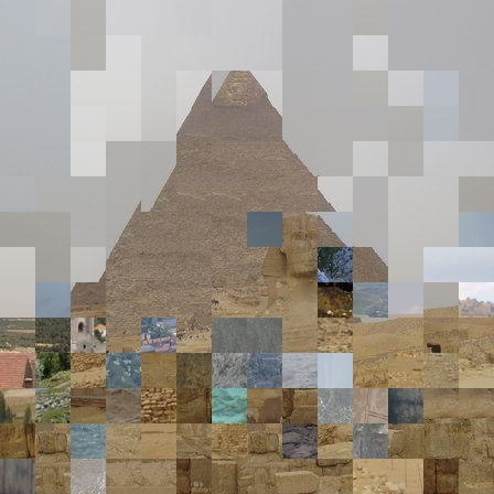
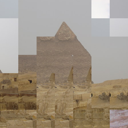
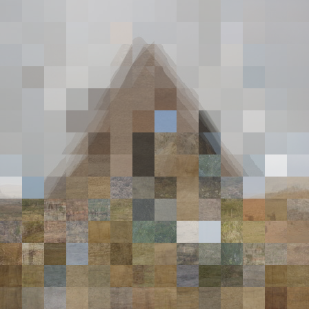
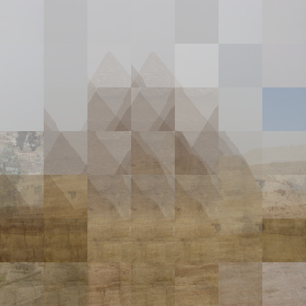
Correspondence visualization. We construct a visualization to observe the correspondence behavior following [18]. To produce the visualization, we first represent each convolutional feature regarding a layer in the database by a square image patch which is obtained from the center of the image region that affects the local feature. Specifically, for an image with a layer output size , each local feature will be represented by a square image patch of size . For each convolutional feature, the original image patch will be replaced by the average of its nearest neighbors from all patches extracted in the database. If the local distinction has been abstracted by high level abstraction, locally different image patches will have similar neighbors as these patches may be semantically close; otherwise the neighbors can be also different since the local distinction is preserved. Note that although the actual image region that affects the local features is much larger than the displayed patch itself due to stacked convolutions, the center patch still preserves localized correspondence [18].
The intermediate convolutional layers of the shallow AlexNet [17] preserve correspondence between different instance objects as well as traditional SIFT descriptor [18]. However, as CNNs become deeper, it is unclear how the intermediate to high level convolutional layers would perform in capturing correspondence information. In addition, we observe the behavior difference between scales of the feature from the visualization. In particular, we would like to understand why the higher layers at finer scale obtain better performance than at lower scale. [18] focuses on part correspondence across different object instances, which is in contrast to our goal of finding correspondence between objects. However, we believe part correspondence is an important step for achieving instance correspondence, and this visualization is also useful in understanding the CNN features in instance correspondence.
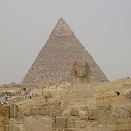
The visualization is presented in Figure 3. The size of the convolutional feature map in Inception 5b scale 1 is , which is much smaller than in Inception 4a’s . Therefore, each patch of Inception 5b in the visualization is much larger than Inception 4a. From the visualization, it is clear that features from Inception 5b do not correspond well compared to those from Inception 4a. In Inception 5b, we can see many repetitive patterns for both 1-NN and 5-NN cases, which means that local features spatially close to each other are highly similar while the local appearance disparity between them is blurred by convolution operations. One possible reason is that GoogLeNet is trained with average pooling just before softmax, which encourages the features of the last convolutional layer to be similar. Comparing Inception 5b (scale 2) to Inception 4a, which have the same feature map sizes, Inception 5b retrieves more semantically relevant rather than locally distinct patches. When applied to finer scale (scale 2), Inception 5b contains more local appearance details than the original scale, thus producing more diverse patches and roughly preserving the original appearance of the objects. The visualization of Inception 4a contains more semantically irrelevant patches, especially in textureless regions, like retrieving grass or sea patches in the pyramid. However, there are less repetitive patterns in the visualization, and the edges in the images are better preserved. This shows that, as an intermediate convolutional layer, Inception 4a is more powerful at preserving correspondence of objects and capturing local appearance distinctions.
Patch clusters. To better observe the clustering of local CNN features, we sample patches in the dataset and show their nearest neighbors on different layers. Each convolutional feature is represented as a patch in the same way as in the correspondence visualization. Figure 4 shows the patch clustering visualization of GoogLeNet layers Inception 3a, Inception 5b and Inception 5b (scale 2). The patch clusters in the lower layer Inception 3a are quite similar to SIFT-like low level features, where strong edges, corners and texture are discovered and encoded. For higher layers, such as Inception 5b, we can see more generalization of parts with semantic meaning, such as different views of a car or scene, which reflects the tendency of higher layers to capture category-level invariances. However, for the same layer Inception 5b applied to the finer scale, the features focus on smaller parts of the images, thus capturing more local appearance. This confirms that the features behave quite differently when applied to images of different resolutions. Although the higher layers are supposed to encode high level categorical features, more instance-level details are also preserved when they are applied to finer scales, so they are more useful for image retrieval.


| Method | Holidays | Oxford | Paris |
|---|---|---|---|
| SIFT-based method | |||
| BoW 200k-D [11] | 54.0 | 36.4 | 46.0 |
| Improved Fisher [21] | 62.6 | 41.4 | - |
| LCS+RN [5] | 65.8 | 51.7 | - |
| VLADintra+ RootSIFT [2] | 65.3 | 55.8 | - |
| CVLAD [35] | 82.7 | 51.4 | - |
| CNN-based method | |||
| CNNaug-ss [25] | 84.3 | 68.0 | 79.5 |
| Multi-resolution | 89.7 | 84.4 | 85.3 |
| Spatial Search [26] | |||
| Neural codes [3] | 79.3 | 54.5 | - |
| MOP-CNN [8] | 80.2 | - | - |
| Ours (OxfordNet) | 83.8 | 64.9 | 69.4 |
| Ours (GoogLeNet) | 84.0 | 58.1 | 68.8 |
4.4 Comparison to state-of-the-art
Since our method only uses simple CNN features and VLAD encoding, we only compare to other recent CNN based approaches and classic SIFT-based representations with BoW and VLAD encoding.
Uncompressed representation. We first compare our approach using uncompressed VLAD representation with other state-of-the-art approaches in Table 2. In Figure 2, the best performing layers on Holidays, Oxford and Paris datasets are Inception 3a on original scale (scale 1), Inception 5b and Inception 4e on finer scale (scale 2) on GoogLeNet respectively, and conv4_2, conv5_1 and conv5_2 for Holidays, Oxford and Paris dataset on OxfordNet respectively. The VLAD descriptors from the two scales on the best performing layer are concatenated as our final multi-scale descriptors. OxfordNet, which has much larger convolutional feature maps, performs slightly better than GoogLeNet for image retrieval. Although we do not focus on producing state-of-the-art results on image retrieval but more on investigating the behavior of convolutional features from different layers and the effect of multiple scales, our system gives competitive results compared to state-of-the-art methods. Specifically, our approach significantly outperforms all the classic SIFT-based approaches with BoW and VLAD encoding, which verifies the representative power of the convolutional features compared to traditional SIFT descriptors. Although better results are reported by other SIFT-based approaches using large vocabularies, spatial verification and query expansion, etc., our framework is not limited to the current setting, and can be readily adapted to other encoding schemes (i.e., BoW and FV), and re-ranking techniques (i.e., query expansion). In addition, compared to recent CNN-based approaches, our method still produces better or comparable results. In particular, our approach outperforms its rivals that either use time-consuming multi-scale sliding windows to extract features [8] or retrain the entire network using extra data [3]. It should be noted that including spatial information greatly boosts the performance of CNN-based approaches such as spatial search [25, 26]. Although [25] and [26] produce better results than our method, we believe that our approach of extracting and encoding convolutional features using lower layers and our investigation of how scales affect convolutional features provide a better understanding of why spatial search on multi-scale features from the last layer performs well. Spatial information can be also included in our framework with few modifications, which will be studied in future work. It would also be interesting to combine multiple layers from the best scales in spatial search to fully utilize the power of deep networks.
| Method | dim | Holidays | Oxford | Paris |
|---|---|---|---|---|
| VLADintra+SIFT [2] | 128 | 62.5 | 44.8 | - |
| FV+T-embedding [12] | 128 | 61.7 | 43.3 | - |
| Neural codes [3] | 128 | 78.9 | 55.7 | - |
| MOP-CNN [8] | 512 | 78.4 | - | - |
| Spatial Pooling [26] | 256 | 74.2 | 53.3 | 67.0 |
| Ours (OxfordNet) | 128 | 81.6 | 59.3 | 59.0 |
| Ours (GoogLeNet) | 128 | 83.6 | 55.8 | 58.3 |
Low-dimensional representation. To trade-off between retrieval accuracy and storage space, most approaches compress the original feature vector to a low-dimensional representation. Therefore, we conduct additional experiments using compressed VLAD descriptors and compare the results with those of other approaches using low-dimensional representations. We use PCA to reduce the dimensionality to 128 and apply whitening to further remove noise.
As shown in Table 3, our method obtains state-of-the-art results on two out of three datasets with minimal performance loss. Our method outperforms all SIFT-based approaches by a large margin, which again demonstrates the power of CNNs. Moreover, we obtain better results than [3], even though [3] fine-tunes the pre-trained CNNs using a large amount of additional data. Although adopting similar VLAD encoding scheme, our method still outperforms MOP-CNN [8] which uses a larger 512-D representation, which further verifies that our approach of extracting convolutional features from intermediate layers is more suitable for instance-level image retrieval. The performance of [26] with low-dimensional descriptors drops notably compared to our 128-D representation, showing that elimination of spatial search greatly reduces the power of CNN representation. It is also important to use more sophisticated encoding methods to capture the local information of convolutional features instead of simple max-pooling as in [26]. In contrast, our low-dimensional representation is robust and retains good discriminative power.
5 Conclusion
In this work, we systematically experiment with features from different layers of convolutional networks and different scales of input images for instance-level image retrieval, and provide insights into performance through various visualizations. With VLAD encoding on convolutional response, we achieve state-of-the-art retrieval results using low dimensional representations on two of the instance image retrieval datasets.
References
- [1] R. Arandjelović and A. Zisserman. Three things everyone should know to improve object retrieval. In CVPR, pages 2911–2918, 2012.
- [2] R. Arandjelovic and A. Zisserman. All about VLAD. In CVPR, pages 1578–1585, 2013.
- [3] A. Babenko, A. Slesarev, A. Chigorin, and V. Lempitsky. Neural codes for image retrieval. In ECCV, pages 584–599. 2014.
- [4] E. J. Crowley and A. Zisserman. In search of art. In Workshop on Computer Vision for Art Analysis, ECCV, 2014.
- [5] J. Delhumeau, P. H. Gosselin, H. Jégou, and P. Pérez. Revisiting the VLAD image representation. In ACM Multimedia, pages 653–656, 2013.
- [6] J. Donahue, Y. Jia, O. Vinyals, J. Hoffman, N. Zhang, E. Tzeng, and T. Darrell. DeCAF: A deep convolutional activation feature for generic visual recognition. In ICML, pages 647–655, 2014.
- [7] M. Douze, A. Ramisa, and C. Schmid. Combining attributes and fisher vectors for efficient image retrieval. In CVPR, pages 745–752, 2011.
- [8] Y. Gong, L. Wang, R. Guo, and S. Lazebnik. Multi-scale orderless pooling of deep convolutional activation features. In ECCV, pages 392–407. 2014.
- [9] H. Jégou and O. Chum. Negative evidences and co-occurences in image retrieval: The benefit of PCA and whitening. In ECCV, pages 774–787, 2012.
- [10] H. Jégou, M. Douze, and C. Schmid. Hamming embedding and weak geometric consistency for large scale image search. In ECCV, pages 304–317, 2008.
- [11] H. Jégou, F. Perronnin, M. Douze, J. Sánchez, P. Pérez, and C. Schmid. Aggregating local image descriptors into compact codes. IEEE Trans. Pattern Anal. Mach. Intell., 34(9):1704–1716, 2012.
- [12] H. Jégou and A. Zisserman. Triangulation embedding and democratic aggregation for image search. In CVPR, pages 3310–3317, 2014.
- [13] Y. Jia, E. Shelhamer, J. Donahue, S. Karayev, J. Long, R. Girshick, S. Guadarrama, and T. Darrell. Caffe: Convolutional architecture for fast feature embedding. arXiv preprint arXiv:1408.5093, 2014.
- [14] A. Kovashka and K. Grauman. Attribute adaptation for personalized image search. In ICCV, pages 3432–3439, 2013.
- [15] A. Kovashka and K. Grauman. Attribute pivots for guiding relevance feedback in image search. In ICCV, pages 297–304, 2013.
- [16] A. Kovashka, D. Parikh, and K. Grauman. Whittlesearch: Image search with relative attribute feedback. In CVPR, pages 2973–2980, 2012.
- [17] A. Krizhevsky, I. Sutskever, and G. E. Hinton. ImageNet classification with deep convolutional neural networks. In NIPS, pages 1097–1105, 2012.
- [18] J. Long, N. Zhang, and T. Darrell. Do convnets learn correspondence? In NIPS, pages 1601–1609, 2014.
- [19] M. Oquab, L. Bottou, I. Laptev, and J. Sivic. Learning and transferring mid-level image representations using convolutional neural networks. In CVPR, pages 1717–1724, 2014.
- [20] D. Parikh and K. Grauman. Implied feedback: Learning nuances of user behavior in image search. In ICCV, pages 745–752, 2013.
- [21] F. Perronnin, Y. Liu, J. Sánchez, and H. Poirier. Large-scale image retrieval with compressed fisher vectors. In CVPR, pages 3384–3391, 2010.
- [22] J. Philbin, O. Chum, M. Isard, J. Sivic, and A. Zisserman. Object retrieval with large vocabularies and fast spatial matching. In CVPR, pages 1–8, 2007.
- [23] J. Philbin, O. Chum, M. Isard, J. Sivic, and A. Zisserman. Lost in quantization: Improving particular object retrieval in large scale image databases. In CVPR, 2008.
- [24] M. Rastegari, A. Diba, D. Parikh, and A. Farhadi. Multi-attribute queries: To merge or not to merge? In CVPR, pages 3310–3317, 2013.
- [25] A. S. Razavian, H. Azizpour, J. Sullivan, and S. Carlsson. Cnn features off-the-shelf: an astounding baseline for recognition. In CVPR Workshops, pages 512–519, 2014.
- [26] A. S. Razavian, J. Sullivan, A. Maki, and S. Carlsson. Visual instance retrieval with deep convolutional networks. CoRR, abs/1412.6574, 2014.
- [27] P. Sermanet, D. Eigen, X. Zhang, M. Mathieu, R. Fergus, and Y. LeCun. Overfeat: Integrated recognition, localization and detection using convolutional networks. CoRR, abs/1312.6229, 2013.
- [28] B. Siddiquie, R. S. Feris, and L. S. Davis. Image ranking and retrieval based on multi-attribute queries. In CVPR, pages 801–808, 2011.
- [29] K. Simonyan and A. Zisserman. Very deep convolutional networks for large-scale image recognition. CoRR, abs/1409.1556, 2014.
- [30] J. Sivic and A. Zisserman. Video Google: A text retrieval approach to object matching in videos. In ICCV, pages 1470–1477, 2003.
- [31] C. Szegedy, W. Liu, Y. Jia, P. Sermanet, S. Reed, D. Anguelov, D. Erhan, V. Vanhoucke, and A. Rabinovich. Going deeper with convolutions. CoRR, abs/1409.4842, 2014.
- [32] J. Wan, D. Wang, S. C. H. Hoi, P. Wu, J. Zhu, Y. Zhang, and J. Li. Deep learning for content-based image retrieval: A comprehensive study. In ACM Multimedia, pages 157–166, 2014.
- [33] Z. Xu, Y. Yang, and A. G. Hauptmann. A discriminative CNN video representation for event detection. arXiv preprint arXiv:1411.4006, 2014.
- [34] M. D. Zeiler and R. Fergus. Visualizing and understanding convolutional networks. In ECCV, pages 818–833, 2014.
- [35] W. Zhao, G. Gravier, and H. Jégou. Oriented pooling for dense and non-dense rotation-invariant features. In BMVC, 2013.