Cooperative Emission of a Pulse Train in an Optically Thick Scattering Medium

Abstract

An optically thick cold atomic cloud emits a coherent flash of light in the forward direction when the phase of an incident probe field is abruptly changed. Because of cooperativity, the duration of this phenomena can be much shorter than the excited lifetime of a single atom. Repeating periodically the abrupt phase jump, we generate a train of pulses with short repetition time, high intensity contrast and high efficiency. In this regime, the emission is fully governed by cooperativity even if the cloud is dilute.

The seminal work on superradiance of R. Dicke in 1954 has opened up tremendous interest in studying cooperative emission of electromagnetic radiation from an ensemble of radiative dipoles (see Dicke (1954) for the original proposal, Gross and Haroche (1982); Brandes (2005) for reviews and Paradis et al. (2008); Das et al. (2008); Scully and Svidzinsky (2009); Ariunbold et al. (2010); Bohnet et al. (2012); Ott et al. (2013); Mlynek et al. (2014) for recent related works). In his original proposal, R. Dicke considered an ensemble of $N$ excited two-level atoms confined inside a volume smaller than $\lambda^{3}$, where $\lambda$ is the transition wavelength. In this context, a macroscopic polarization is built up in the medium upon incoherent spontaneous emission. This Dicke superradiance mechanism leads to the coherent emission of an intense pulse with a decay time, $\tau_{D}=(N\Gamma)^{-1}$, that is shortened by a factor of $N^{-1}$ with respect to the atomic excited state lifetime, $\Gamma^{-1}$. For practical implementation in the optical domain, the Dicke model was extended to media with volume larger than $\lambda^{3}$ Rehler and Eberly (1971); Bonifacio and Lugiato (1975); Gross and Haroche (1982). In those cases, the propagation of the electromagnetic field in the medium and the spatial mode density must be taken into account. If the medium is dense, i.e., $\rho\lambda^{3}\gg 1$, where $\rho$ is the radiator spatial density, it still exhibits the main feature of the Dicke superradiance, namely, the emission of a short pulse after some delay Skribanowitz et al. (1973); Marek (1979); Paradis et al. (2008); Ariunbold et al. (2010). It was, however, pointed out in Rehler and Eberly (1971), that the superradiant pulse decay time should be corrected as $\tau=\tau_{D}/\mu$. $\mu<1$ is a geometrical factor corresponding to the solid angle subtended by the superradiant emission Gross and Haroche (1982); Bonifacio and Lugiato (1975).

For a dilute scattering medium, i.e., $\rho\lambda^{3}\ll 1$, the Dicke superradiance mechanism does not occur Note (1). Nevertheless, an optically thick medium driven by a coherent incident field shares interesting similarities with Dicke superradiance; here, the cooperativity factor $N\mu$ is replaced by the optical thickness of the medium Friedberg and Hartmann (1971, 1976). Once a driving coherent field is abruptly switched off, like in a free induction decay (FID) experiment Hahn (1950); Brewer and Shoemaker (1972); Foster et al. (1974); Toyoda et al. (1997); Shim et al. (2002); Wei et al. (2009); Chalony et al. (2011); Kwong et al. (2014), a short coherent cooperative flash of light is emitted in the forward direction. The flash duration is inversely proportional to the optical thickness and the bare linewidth of the transition Chalony et al. (2011). A similar phenomenon occurs for the optical precursor, i.e., when the driving coherent field is abruptly switched on Jeong et al. (2006).

In a coherently driven medium, the incident probe frequency can be detuned with respect to the atomic resonance, leading to a nontrivial phase rotation of the cooperatively emitted field (see Kwong et al. (2014) in the optical domain and Helistö et al. (1991); Shakhmuratov et al. (2015); Antonov et al. (2015) for $\gamma$-ray pulses in Mössbauer spectroscopy experiments). In this Letter, we report the generation of high repetition rate and high intensity contrast pulse trains in an optically thick cold dilute atomic ensemble using the setup schematically shown in Fig. 1(a). An example of a pulse train, generated in our experiment by periodically changing the probe phase, is shown in Fig. 1(b). As a consequence of cooperative emission, the repetition time $T_{R}$ of the pulse train can be shorter than the atomic excited state lifetime, $\Gamma^{-1}$. Moreover, we show that at high repetition rate, the single atom fluorescence is quenched. This constitutes a rather counterintuitive result where the emission in free space is fully governed by cooperativity, in contrast with the usual situations where it is enhanced by a cavity surrounding the medium Carmichael et al. (1991).

Figure 1: (color online). (a) Experimental setup: a laser beam is sent through an acousto-optic modulator (AOM), which may be used to switch on and off the incident beam, followed by an electro-optic modulator (EOM), which abruptly changes the phase of the incident probe field, $E_{0}$. (b) A pulse train generated at a repetition time of $T_{R}=0.12\Gamma^{-1}$ by a periodic abrupt phase change of $\pi$. Here, the probe laser is at resonance. (c) Electric fields just before and just after an abrupt phase jump of $\pi$ are represented schematically in the complex plane. Before the phase jump, the forward scattered field $E_{s}$ destructively interferes with $E_{0}$. After the phase jump, they constructively interfere. The transmitted field is denoted by $E_{t}$.

The scattering medium is a cloud of laser-cooled ⁸⁸Sr atoms (see Yang et al. (to be published) and Kwong et al. (2014) for the details of the cold atoms production line). The ellipsoidal shape of the cold cloud has an axial radius of $240(10)\text{\,}\mathrm{\SIUnitSymbolMicro m}$ and an equatorial radius of $380(30)\text{\,}\mathrm{\SIUnitSymbolMicro m}$, with peak density around $4.6\times 10^{11}\text{\,}\rpcubic{\mathrm{c}\mathrm{m}}$ for a total of $2.5(5)\times 10^{8}$ atoms. $\lambda=$689\text{\,}\mathrm{nm}$$ is the wavelength associated to the ${}^{1}\!S_{0}\rightarrow\,^{3}\!P_{1}$ intercombination line (bare linewidth of $\Gamma/2\pi=$7.5\text{\,}\mathrm{kHz}$$) used in this experiment. $\rho\lambda^{3}=0.15$, which puts us in the dilute regime. The temperature of the cold gas is $T=$3.3(2)\text{\,}\mathrm{\SIUnitSymbolMicro K}$$. We get $k\mathrm{bar}{v}=3.4\Gamma$, indicating a significant Doppler broadening of the narrow intercombination line. $k=2\pi/\lambda$ is the wave vector of the transition, and $\mathrm{bar}{v}$ is the rms velocity of the gas. The optical thickness depends strongly on the temperature. We measure $19(2)$ along the equatorial axis at resonance.

A 150 $\mu$m diameter probe laser beam, tuned around the intercombination line, is sent through the cold atomic gas along an equatorial axis. The probe power is $400(40)\text{\,}\mathrm{pW}$, corresponding to $0.45(5)I_{\mathrm{sat}}$ (${I_{\mathrm{sat}}=3\leavevmode\nobreak\ \mu\text{W/cm}^{2}}$). We measure the forward transmitted intensity of the probe using a photodetector, integrating over the transverse dimensions of the transmitted beam. We apply a bias $1.4\text{\,}\mathrm{G}$ magnetic field along the beam polarization during the probing phase, making the atom an effective two-level system on the ${}^{1}\!S_{0},m=0\rightarrow\,^{3}\!P_{1},m=0$ transition.

The ellipsoidal shape of the cloud is modeled by a slab geometry, so that the coherent transmitted electric field, in the frequency domain, is given by

$$E_{t}(\omega)=E_{0}(\omega)\exp\left[i\frac{n(\omega)\omega L}{c}\right].$$ (1)

In the above equation, $n(\omega)$, $E_{0}$, $c$, and $L$ are the complex effective refractive index, the incident optical field, the speed of light in vacuum, and the slab thickness along the laser beam, respectively. For a dilute medium, $n(\omega)=1+\rho\alpha(\omega)/2$ Hetch and Zajac (1974), with the two-level atomic polarizability,

$$\alpha(\omega)=-\frac{3\pi\Gamma c^{3}}{\omega^{3}}\frac{1}{\sqrt{2\pi}\mathrm{bar}{v}}\int^{+\infty}_{-\infty}dv\frac{\textrm{exp}\left(-v^{2}/2\mathrm{bar}{v}^{2}\right)}{\delta-kv+i\Gamma/2}.$$ (2)

$\delta=\omega-\omega_{0}$ is the detuning of the probe laser frequency $\omega$ with respect to the bare atomic resonance frequency, $\omega_{0}$. The effect of Doppler broadening is included in the polarizability by averaging over the thermal Gaussian distribution of the atomic velocity $v$ along the beam propagation direction. The transmitted intensity $I_{t}(t)$ is computed following Kwong et al. (2014), and by performing an inverse Fourier transform. We define, for given $\delta$ and $\mathrm{bar}{v}$, the optical thickness $b_{\mathrm{bar}{v}}(\delta)$ and the relative phase $\theta_{\mathrm{bar}{v}}(\delta)$ between the transmitted and the incident fields by

$$b_{\mathrm{bar}{v}}(\delta)=\, \frac{2\omega}{c}\operatorname{Im}[n(\omega)]L,$$

$$\theta_{\mathrm{bar}{v}}(\delta)=\, \frac{\omega}{c}\operatorname{Re}[n(\omega)-1]L.$$ (3)

The transmitted field $E_{t}$ results from the interference between the incident field $E_{0}$ and the field scattered in the forward direction $E_{s}$,

$$E_{t}=E_{0}+E_{s}.$$ (4)

For effective two-level atoms, we can drop the vectorial nature of the electric fields and represent them as scalar quantities. Because of the noninstantaneous response time of the medium, the coherent scattered field in the forward direction is a continuous function across the abrupt change of the incident field. In a FID experiment where the incident field is abruptly switched off at $t=0$, the intensity of the transmitted field at $t=0^{+}$ is a direct measurement of the forward scattered intensity in the stationary regime. Its properties are studied in detail in  Chalony et al. (2011); Kwong et al. (2014). In particular, the intensity of the forward scattering is bounded by 4 times the incident intensity (“superflash effect”) Kwong et al. (2014). The temporal evolution of the transmitted field, after the abrupt switch off of the incident field, is not a simple function having only one characteristic decay rate Chalony et al. (2011). However, we get a clear physical insight by considering only the initial decay time (at $t=0^{+}$), which takes a simple analytical expression (see Supplemental Material  Note (2)):

$$\tau_{\mathrm{bar}{v}}(\delta)=\left|\frac{I_{t}(t=0^{+})-I_{t}(t=\infty)}{dI_{t}/dt(t=0^{+})}\right|\\ =\frac{2}{\Gamma b_{0}(0)}\frac{1+\exp(-b)-2\exp(-b/2)\cos(\theta)}{1-\exp(-b/2)\cos(\theta)}$$ (5)

where $b\equiv b_{\mathrm{bar}{v}}(\delta)$ and $\theta\equiv\theta_{\mathrm{bar}{v}}(\delta)$. In Eq. (5), $b_{0}(0)$ is the optical thickness at resonance and zero velocity. It is linked to $b_{\mathrm{bar}{v}}(0)$ by $b_{\mathrm{bar}{v}}(0)=b_{0}(0)g(k\mathrm{bar}{v}/\Gamma)$ where $g(x)=\sqrt{\pi/8}\exp\left(1/8x^{2}\right)\operatorname{erfc}\left(1/\sqrt{8}x\right)/x$ Chalony et al. (2011).

For small optical thickness, Eq. (5) reduces to $\tau_{\mathrm{bar}{v}}(0)=g(k\mathrm{bar}{v}/\Gamma)/\Gamma$ at resonance. It is shorter than $\tau_{0}(0)=1/\Gamma$ due to the dephasing effect from the motion of the atoms. This has already been observed experimentally [see Fig. 3(b) of Chalony et al. (2011) where the transition is Doppler broadened, and Fig. 5 of Shim et al. (2002) where Doppler broadening can be ignored]. In our experiments, $g(k\mathrm{bar}{v}/\Gamma)\approx 0.16$; thus, for $b_{\mathrm{bar}{v}}(0)=19(2)$, we get $b_{0}(0)=120(10)$. A direct measurement gives a slightly smaller value, $b_{0}(0)=95(5)$ (see Supplemental Material Note (2)). The expression of $\tau_{\mathrm{bar}{v}}$, given by Eq. (5), simplifies to $\tau_{\mathrm{bar}{v}}(0)=2[b_{0}(0)\Gamma]^{-1}$ at resonance ($b\gg 1$, $\theta=0$) and to $\tau_{\mathrm{bar}{v}}(\pm\infty)=4[b_{0}(0)\Gamma]^{-1}$ far from resonance ($b=0$ and $\theta=0$). The solid blue curve in Fig. 2 is a plot of $\tau_{\mathrm{bar}{v}}(\delta)$ for $k\mathrm{bar}{v}/\Gamma=3.4$. $\tau_{\mathrm{bar}{v}}$ has a weak dependence on $\delta$ and $\mathrm{bar}{v}$; it depends mainly on $b_{0}(0)$, which can be much larger than the optical thickness $b_{\mathrm{bar}{v}}(0)$ seen by a resonant probe at nonzero temperature. This strongly reduces the lifetime of the forward scattered field with respect to the atomic lifetime, $\Gamma^{-1}$. Equation (5) has a rather simple physical interpretation: the second term represents the geometrical properties of the propagation inside the medium (change in amplitude and phase shift) while the term $2/\Gamma b_{0}(0)$ represents the collective behavior of all excited dipoles. It does not depend on the atomic velocity, but only on the atomic density integrated along the laser direction, because there is no Doppler effect for photons scattered in the forward direction. Similarly, it does not depend on the detuning because all dipoles decay with the same rate $\Gamma$ independently of the detuning.

The FID experiment is performed using an AOM as a light switching device [see Fig 1(a)]. The experimental data points, represented by blue open circles in Fig. 2, are in reasonable agreement with the theoretical prediction. The evaluation of $dI_{t}/dt(t=0^{+})$ is performed on a short temporal window ($\sim$200\text{\,}\mathrm{ns}$$) after switching off the incident probe. While the flash signal has a good signal to noise ratio [see Fig. 1(b)], the resulting $dI_{t}/dt(t=0^{+})$ values from this analysis are noisier. This leads to the large statistical errors for $\tau_{\mathrm{bar}{v}}$. The slight positive systematic error, also associated to the determination of $dI_{t}/dt(t=0^{+})$, comes from the finite response time of our experimental scheme, of the order of $$40\text{\,}\mathrm{n}\mathrm{s}$\approx(500\Gamma)^{-1}$. To check the latter statement, we use Eqs. (1) and (2) to numerically compute $I_{t}(t).$ $E_{0}(\omega)$ in Eq. (1) is determined from the measured time evolution of the incident intensity. We then apply, on the numerical signal, the same procedure used experimentally to extract $\tau_{\mathrm{bar}{v}}$, resulting in an excellent agreement with the experimental data (see Fig. 2).

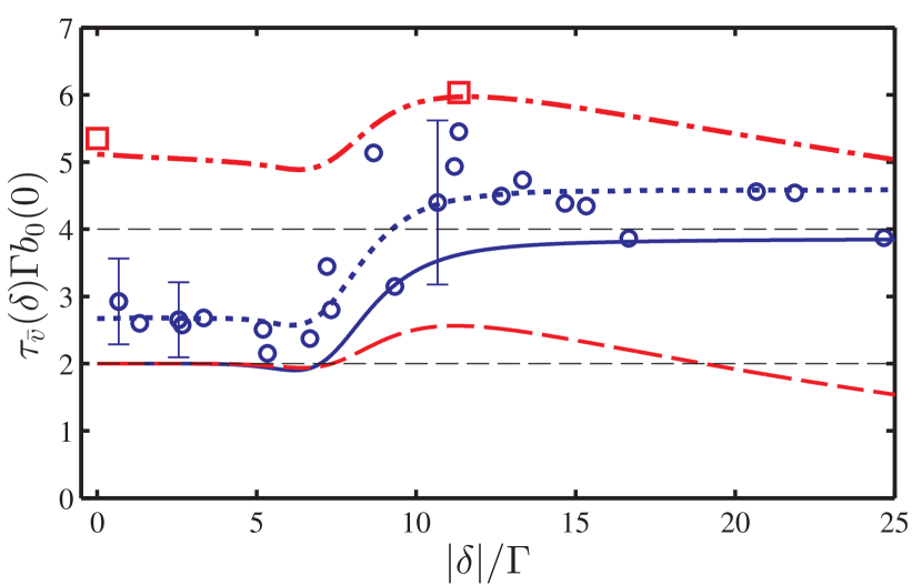
Figure 2: (color online). Initial decay time of the coherent flash versus the probe detuning at $k\mathrm{bar}{v}/\Gamma=3.4$. The zero temperature resonant optical thickness is $b_{0}(0)=120$. The blue open circles and plain curve are, respectively, the experimental data points and the theoretical curve for an abrupt switch off of the probe. The two horizontal black dashed lines give the theoretical predictions at resonance and at large detuning. The red squares and dashed curve are the experimental data points and theoretical prediction for an abrupt phase jump of $\pi$. The blue dotted line and the red dash-dotted line are numerical predictions taking into account the finite response time of the experimental scheme (see text for more details).

Instead of a FID experiment, we now consider an abrupt jump of the phase of the incident field by $\pi$ [see Fig. 1(c)], at constant incident intensity. The initial decay time $\tau_{\mathrm{bar}{v}}$ becomes (see Supplemental Material Note (2)):

$$\tau_{\mathrm{bar}{v}}(\delta)=\frac{4}{\Gamma b_{0}(0)}\frac{1-\exp(-b/2)\cos\theta}{2-\exp(-b/2)\cos\theta}.$$ (6)

We plot this expression as the red dashed line in Fig. 2. If the $\pi$ phase jump occurs at $t=0$, according to Eq. (4), we have $E_{t}(t=0^{+})=-E_{0}(t=0^{-})+E_{s}(t=0^{-})$. To observe the largest possible amplitude of the transient field, we choose the probe frequency detuning such that the interference between $E_{0}(t=0^{-})$ and $E_{s}(t=0^{-})$ is destructive. This condition is necessarily fulfilled when the incident field is at resonance. If $b_{\mathrm{bar}{v}}(0)\gg 1$, $|E_{s}(t=0^{-})|\simeq|E_{0}|$, so we expect a coherent flash with a peak intensity, $I_{t}=4I_{0}$. The destructive interference condition may also happen at a nonzero detuning if the phase rotation experienced by $E_{s}$ is large enough, for example if $b_{\mathrm{bar}{v}}(0)\gg 1$. In our experiment, this situation occurs at $|\delta|=11.3\Gamma$ (i.e., superflash regime Kwong et al. (2014)). In this context, $|E_{s}(t=0^{-})|\simeq 1.8|E_{0}|$; thus, the flash has a peak intensity $I_{t}\simeq(1+1.8)^{2}I_{0}\simeq 7.8I_{0}$. This value is slightly below the maximum value $9I_{0}$ allowed by energy conservation, achievable at larger optical thickness.

The phase jump is performed using an EOM placed on the probe laser path [see Fig. 1(a)]. The EOM is driven by a high voltage controller and has a slew rate $\sim 2.3\pi\leavevmode\nobreak\ \text{rad }\mu\text{s}^{-1}$. The two experimental values (red squares), corresponding to $\delta=0$ and $|\delta|=11.3\Gamma$, are shown in Fig. 2. They are systematically higher than the theoretical prediction for an abrupt phase shift change because of the response time of the EOM driver. Similarly to the FID experiment, we use the experimentally measured EOM driver output to numerically compute the $I_{t}(t)$ signal. The resulting values of the decay time (red dash-dotted line in Fig. 2) agree with the experimental ones.

We now analyze the cooperative emission when a square periodic $\pi$ phase jump is applied. We observe a pulse train with a repetition time $T_{R}$ [see an example in Fig. 1(b)] limited by the relaxation time of the system. The cooperative emission in the forward direction dramatically decreases the repetition time below the atomic excited state lifetime.

Bringing the probe on resonance, we plot in Fig. 3(a) (red dots and solid curve) the intensity contrast $I_{c}$ of the pulse train. We define $I_{c}=\operatorname{max}\{I_{t}\}-\langle I_{t}\rangle$ as the difference between the maximum intensity $\operatorname{max}\{I_{t}\}$ and the mean intensity, $\langle I_{t}\rangle=1/T_{R}\int_{T_{R}}I_{t}(t)dt$. We observe an excellent agreement between the experiment and the theoretical prediction of Eqs. (1) and (2). At long repetition time, i.e., $T_{R}\gg\Gamma^{-1}$, the system reaches its steady state before every phase jump. Hence, we measure $I_{c}\simeq 4I_{0}-\langle I_{t}\rangle\simeq 4I_{0}$. We note that $\langle I_{t}\rangle\simeq 0$ [see the blue open circles and dashed curve in Fig. 3(a)] and most of the incident power is scattered out by single atom fluorescence events. In the $\tau_{\mathrm{bar}{v}}\lesssim T_{R}\lesssim\Gamma^{-1}$ intermediate regime, $I_{c}$ oscillates and can reach a larger value. Moreover, the mean intensity $\langle I_{t}\rangle$ rapidly increases to its maximal value, $I_{0}$. Here, the incident power is almost perfectly transferred to the pulse train. This interesting result can be understood considering cooperativity in forward scattering. Indeed, its characteristic relaxation time scales like $[b_{0}(0)\Gamma]^{-1}$. Therefore, for $b_{0}(0)\gg 1$, coherent processes relax much faster than single atom fluorescence events. The latter are quenched, leading to the good figure of merit at a repetition time shorter than $\Gamma^{-1}$. In other words, the emission from the atoms is governed by cooperativity. For $T_{R}<\tau_{\mathrm{bar}{v}}$, the repetition rate is faster than any time scale of the atomic ensemble. Even though the probe power is fully transmitted, the contrast $I_{c}$ tends to zero.

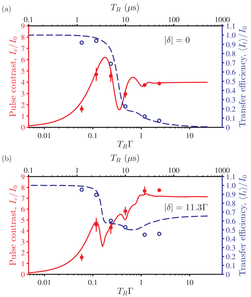
Figure 3: (color online). Figures of merit of the generated pulse train (a) at resonance and (b) at $|\delta|=11.3\Gamma$. The red solid and blue dashed curves are the theoretical predictions for the intensity contrast $I_{c}/I_{0}$ and transfer efficiency $\langle I_{t}\rangle/I_{0}$, respectively. The red dots and blue open circles are the corresponding experimentally measured values.

At detuning $|\delta|=11.3\Gamma$, for long repetition time ($T_{R}\gg\Gamma^{-1}$), the pulses have a higher contrast, $I_{c}\simeq(1+1.8)^{2}I_{0}-\langle I_{t}\rangle\simeq 7.1I_{0}$ [see Fig. 3 (b)]. The large value of the mean intensity, namely, $\langle I_{t}\rangle\simeq 0.7I_{0}$, is due to the small optical thickness, $b_{\mathrm{bar}{v}}(\delta)=0.4$. Hence, most of the transmitted power is in a continuous transmission mode and not in the pulse train. At the intermediate repetition time ($\tau_{\mathrm{bar}{v}}\lesssim T_{R}\lesssim\Gamma^{-1}$), the pulse contrast and the figure of merit are not as good as in the resonant case.

To conclude, we generate pulse trains of short repetition time using cooperative forward emission in an optically thick scattering medium. We can almost completely transfer the incident power into the high intensity contrast pulse train, quenching the single atom fluorescence. This means that, in free space, the cooperativity effect can dominate emission from a dilute atomic gas. The decay time of the pulses also weakly depends on the temperature of the gas and on the probe detuning. An interesting extension of this study could be to look for quantum signatures in the cooperative emission.

Finally, we employ the narrow intercombination line of strontium as a proof of principle, where the time scales are of the order of microseconds. For future practical applications, such as a high contrast pulse generator, shorter repetition times in the picosecond or subpicosecond regime should be attainable. For this purpose, one has to use scattering media with higher optical thickness and/or shorter transition lifetime. The fact that cooperativity is robust over thermal dephasing means that we can also use a hot vapor of rubidium [$b_{\mathrm{bar}{v}}(0)\approx 600$ at $110\text{\,}\mathrm{\SIUnitSymbolCelsius}$ Weller et al. (2011)]. We can also use condensed matter systems, e.g., a samarium doped fiber [$b(0)\approx 100$ Luo and Chu (1999)], which allows us to bring this technique into the 1.55 $\mu$m telecommunication band.

The authors thank M. Pramod, F. Leroux, and K. Pandey for technical support and fruitful discussions. C. C. K. thanks the CQT and ESPCI institutions for funding his trip to Paris. This work was supported by CQT/MoE funding, Grant No. R-710-002-016-271. R. P. acknowledges the support of LABEX WIFI (Laboratory of Excellence ANR-10-LABX-24) within the French Program “Investments for the Future” under reference ANR-10-IDEX-0001-02 PSL^∗.

Supplemental Material

Optical thickness measurement

We employ three different methods to measure the optical thickness. First, we compute the theoretical transmission spectrum for various $b_{\mathrm{bar}{v}}(\delta)$ values and use these profiles to fit the experimentally obtained transmission data. This leads to an optical thickness $b_{\mathrm{bar}{v}}(0)=19$. Second, we perform a shadow imaging experiment on the ${}^{1}S_{0}\,\rightarrow\,^{1}P_{1}$ broad transition ($\lambda_{b}=$461\text{\,}\mathrm{nm}$$, linewidth $\Gamma_{b}=$2\pi\times 32\text{\,}\mathrm{MHz}$$), where Doppler broadening is negligible. A collimated probe beam with a waist larger than the atomic cloud is sent onto the cloud, and the transmission signal $I_{t}/I_{0}$ is measured using an electron multiplying CCD camera (Andor iXon Ultra 897). Typically, the probe frequency is set at a detuning, $\delta_{b}=$53\text{\,}\mathrm{MHz}$$, to reduce the systematic error in the transmission measurement due to large optical thickness. The optical thickness $\mathcal{B}$ is computed from the transmission signal, $\mathcal{B}=-\log(I_{t}/I_{0})$, and is related to $b_{0}(0)$ of the intercombination line by $b_{0}(0)=\mathcal{B}\left(1+4\delta_{b}^{2}/\Gamma_{b}^{2}\right)\lambda^{2}/\lambda_{b}^{2}$. In our experiment, we measure a peak value of $b_{0}(0)=95(5)$ using this method and a corresponding value of $b_{\mathrm{bar}{v}}(0)=15(1)$ using $b_{\mathrm{bar}{v}}(0)=b_{0}(0)g(k\mathrm{bar}{v}/\Gamma)$. Third, we carry out shadow imaging experiment directly on the intercombination line transition. We vary the detuning in a range of 100 kHz around the resonance. The value of $b_{\mathrm{bar}{v}}(0)$ is deduced using

$$E_{t}(\omega)=E_{0}(\omega)\mathrm{e}^{i\frac{n(\omega)\omega L}{c}},$$ (S1)

and

$$\alpha(\omega)=-\frac{3\pi\Gamma c^{3}}{\omega^{3}}\frac{1}{\sqrt{2\pi}\mathrm{bar}{v}}\int^{+\infty}_{-\infty}\mathrm{d}v\frac{\mathrm{e}^{-v^{2}/2\mathrm{bar}{v}^{2}}}{\delta-kv+i\Gamma/2},$$ (S2)

which are Eqs. (1) and (2) in the main text. We have $b_{\mathrm{bar}{v}}(0)=19(2),$ a value slightly larger than the one obtained by the second method.

Initial decay time $\tau_{\mathrm{bar}{v}}$

We take $t=0$ as the time when the abrupt change occurs for the incident field $E_{0}$. To calculate the initial decay time of the cooperative forward transmitted field, we first note that we can rewrite Eq. (5) in the main text as

$$\tau_{\mathrm{bar}{v}}(\delta)=\left|\frac{1-|E_{t}(t=\infty)|^{2}/|E_{t}(t=0^{+})|^{2}}{2\operatorname{Re}\left\{\frac{\mathrm{d}E_{t}/\mathrm{d}t(t=0^{+})}{E_{t}(t=0^{+})}\right\}}\right|,$$ (S3)

where $E_{t}(t=0^{+})=E_{0}(t=0^{+})+E_{s}(t=0^{-})$, and $E_{t}(t=\infty)$ is the steady state transmitted field after the abrupt change in the incident field. For the case of abrupt extinction, $E_{t}(t=0^{+})=E_{s}(t=0^{-})$ and $E_{t}(t=\infty)=0$. For abrupt ignition, $E_{t}(t=0^{+})=E_{0}$ and $|E_{t}(t=\infty)|=|E_{0}|\mathrm{e}^{-b/2}$. Here, $b=b_{v}(\delta)$ and $\theta=\theta_{v}(\delta)$, the same as defined in Eq. (3) of the main text:

$$b_{\mathrm{bar}{v}}(\delta)=\frac{2\omega}{c}\operatorname{Im}[n(\omega)]L,\quad\theta_{\mathrm{bar}{v}}(\delta)=\frac{\omega}{c}\operatorname{Re}[n(\omega)-1]L.$$ (S4)

For abrupt phase jump by $\varphi$, we have $E_{t}(t=0^{+})=E_{0}\mathrm{e}^{i\varphi}+E_{s}(t=0^{-}),$ ignoring the small propagation time $L/c$ in the medium, and $|E_{t}(t=\infty)|=|E_{0}|\mathrm{e}^{-b/2}$. The forward scattered field during the steady state regime, in both cases of abrupt extinction and phase jump, is $E_{s}(t=0^{-})=E_{0}\mathrm{e}^{-b/2+i\theta}-E_{0}$.

In the denominator of Eq. (S3), we need to compute the time derivative of the transmitted field at $t=0^{+}$. It can be computed by considering the derivative $\mathrm{d}\left[E_{s}(t)\mathrm{e}^{i\omega t}\right]/\mathrm{d}t$. The forward scattered field in the time domain, $E_{s}(t)$, is related to the incident field in the frequency domain, $E_{0}(\omega^{\prime})$, by the following well-behaved integral:

$$E_{s}(t)\\ =\int\mathrm{e}^{-i\omega^{\prime}t}\left[\mathrm{e}^{i\frac{\omega^{\prime}\rho\alpha\left(\omega^{\prime}\right)L}{2c}}-1\right]E_{0}(\omega^{\prime})\mathrm{d}\omega^{\prime}.$$ (S5)

The integration ranges of the integrals in this Supplemental Material, when not specified, are from $-\infty$ to $\infty$. $E_{0}(\omega^{\prime})$ is given for the cases of abrupt ignition, abrupt extinction and abrupt phase jump of $\varphi$ by:

$$E_{0}(\omega^{\prime})=\frac{i\xi E_{0}}{2\pi}\mathrm{PV}\frac{1}{\omega^{\prime}-\omega}+\frac{\eta E_{0}}{2}\delta(\omega^{\prime}-\omega).$$ (S6)

where $\omega$ is the frequency of the probe. The Fourier variable corresponding to $t$ is denoted as $\omega^{\prime}$. $\xi$ and $\eta$ are $-1$ and $1$ respectively for abrupt extinction of the probe, and $\mathrm{e}^{i\varphi}-1$ and $1+\mathrm{e}^{i\varphi}$ respectively for abrupt phase jump of the probe field. In the case of abrupt probe ignition, both $\xi$ and $\eta$ are equal to 1. We substitute Eq. (S6) in Eq. (S5), noting that the integral involving the Dirac delta function goes to zero, to obtain

$$\frac{\mathrm{d}}{\mathrm{d}t}\left[E_{s}(t)\mathrm{e}^{i\omega t}\right]\\ =\frac{\xi E_{0}}{2\pi}\sum_{p=1}^{\infty}\frac{1}{p!}\int\left(\frac{i\omega^{\prime}\rho\alpha(\omega^{\prime})L}{2c}\right)^{p}\mathrm{e}^{-i(\omega^{\prime}-\omega)t}\mathrm{d}\omega^{\prime}.$$ (S7)

We work in the regime where $\delta,\Gamma,k\mathrm{bar}{v}\ll\omega_{0}$. For $p=1$, the integral can be evaluated to be

$$\frac{\xi E_{0}}{2\pi}\int\frac{i\omega^{\prime}\rho\alpha(\omega^{\prime})L}{2c}\mathrm{e}^{-i(\omega^{\prime}-\omega)t}\mathrm{d}\omega^{\prime}\\ =\frac{\xi E_{0}}{2\pi i}\frac{b_{0}(0)}{2}\frac{\Gamma}{2}\frac{1}{\sqrt{2\pi}\mathrm{bar}{v}}\iint\mathrm{d}v\,\mathrm{d}\omega^{\prime}\frac{\mathrm{e}^{-i(\omega^{\prime}-\omega)t}\mathrm{e}^{-v^{2}/2\mathrm{bar}{v}^{2}}}{\omega^{\prime}-\omega_{0}-kv+i\Gamma/2}\\ =-\xi E_{0}\frac{b_{0}(0)\Gamma}{4}\mathrm{e}^{i\delta t}\mathrm{e}^{-\Gamma t/2}\frac{1}{\sqrt{2\pi}\mathrm{bar}{v}}\int\mathrm{d}v\,\mathrm{e}^{-ikvt}\mathrm{e}^{-v^{2}/2\mathrm{bar}{v}^{2}}\\ =-\xi E_{0}\frac{b_{0}(0)\Gamma}{4}\mathrm{e}^{i\delta t}\mathrm{e}^{-\Gamma t/2}\mathrm{e}^{-k^{2}\mathrm{bar}{v}^{2}t^{2}/2},$$ (S8)

for $t>0$. In Eq. (S8), $b_{0}(0)=6\pi\rho c^{2}L/\omega_{0}^{2}$. The $p>1$ terms, in general, are difficult to evaluate for the general time dependence. Nevertheless, at $t=0^{+}$, they vanish. We take the example of the term $p=2$, where essentially we have to deal with the following triple integral.

$$\iiint\frac{\mathrm{e}^{-i(\omega-\omega^{\prime})t}\mathrm{e}^{-v^{2}/(2\mathrm{bar}{v}^{2})}\mathrm{e}^{-v^{\prime 2}/(2\mathrm{bar}{v}^{2})}\,\mathrm{d}\omega^{\prime}\mathrm{d}v\,\mathrm{d}v^{\prime}}{(\omega^{\prime}-\omega_{0}-kv+i\Gamma/2)(\omega^{\prime}-\omega_{0}-kv^{\prime}+i\Gamma/2)}.$$ (S9)

We rewrite for $v\neq v^{\prime}$,

$$\frac{\mathrm{e}^{-i(\omega-\omega^{\prime})t}}{(\omega^{\prime}-\omega_{0}-kv+i\Gamma/2)(\omega^{\prime}-\omega_{0}-kv^{\prime}+i\Gamma/2)}\\ =\frac{1}{k(v-v^{\prime})}\frac{\mathrm{e}^{-i(\omega-\omega^{\prime})t}}{\omega^{\prime}-\omega_{0}-kv+i\Gamma/2}\\ -\frac{1}{k(v-v^{\prime})}\frac{\mathrm{e}^{-i(\omega-\omega^{\prime})t}}{\omega^{\prime}-\omega_{0}-kv^{\prime}+i\Gamma/2}.$$ (S10)

The integration over $\omega^{\prime}$ of the above expression can be carried out easily, which results in 0 at $t=0^{+}$. When $v=v^{\prime}$, we have an integral over a multiple pole of order $2$, which also goes to 0 at $t=0^{+}$. Therefore, the term with $p=2$ is zero at $t=0^{+}$. Similar argument can be extended to all orders $p>1$, showing that all $p>1$ terms vanish at $t=0^{+}$. Finally, we have

$$\frac{\mathrm{d}}{\mathrm{d}t}\left[E_{s}(t)\mathrm{e}^{i\omega t}\right](t=0^{+})=-\xi E_{0}\frac{b_{0}(0)\Gamma}{4}.$$ (S11)

We then use the fact that $E_{s}(t=0^{+})=E_{t}(t=0^{+})-E_{0}(t=0^{+})$ to obtain

$$\frac{\mathrm{d}E_{t}}{\mathrm{d}t}(t=0^{+})=-\xi E_{0}\frac{b_{0}(0)\Gamma}{4}-i\omega E_{t}(t=0^{+}).$$ (S12)

Using the above expression, we deduce the initial decay time for the case of abrupt probe extinction,

$$\tau_{\mathrm{bar}{v}}(\delta)=\frac{2}{\Gamma b_{0}(0)}\frac{1+\exp(-b)-2\exp(-b/2)\cos(\theta)}{1-\exp(-b/2)\cos(\theta)},$$ (S13)

which is Eq. (5) of the main text. For the case of abrupt phase change, we find the initial decay time to be

$$\tau_{\mathrm{bar}{v}}(\delta)=\frac{4}{\Gamma b_{0}(0)}\frac{1-\exp(-b/2)\cos\theta}{2-\exp(-b/2)\cos\theta}.$$ (S14)

This is Eq. (6) of the main text. The initial decay time of the flash in the case of abrupt ignition is found to be

$$\tau_{\mathrm{bar}{v}}(\delta)=\frac{2}{\Gamma b_{0}(0)}\left[1-\mathrm{e}^{-b}\right].$$ (S15)

We observe again the appearance of the factor $2/\Gamma b_{0}(0)$ which arises from the cooperativity among the atomic dipoles.

In the case of an abrupt phase jump, we can further choose in the experiment, for $\varphi$ to be equal to the phase of $E_{s}(t=0^{-})$ relative to $E_{0}(t=0^{-})$. This choice ensures a constructive interference after the phase jump. The decay time can be simplified to

$$\tau_{\mathrm{bar}{v}}(\delta)=\frac{4}{\Gamma b_{0}(0)}\frac{|E_{s}(t=0^{+})|}{E_{0}+|E_{s}(t=0^{+})|}.$$ (S16)

References

- Dicke (1954) R. H. Dicke, Phys. Rev. 93, 99 (1954).
- Gross and Haroche (1982) M. Gross and S. Haroche, Phys. Rep. 93, 301 (1982).
- Brandes (2005) T. Brandes, Phys. Rep. 408, 315 (2005).
- Paradis et al. (2008) E. Paradis, B. Barrett, A. Kumarakrishnan, R. Zhang, and G. Raithel, Phys. Rev. A 77, 043419 (2008).
- Das et al. (2008) S. Das, G. S. Agarwal, and M. O. Scully, Phys. Rev. Lett. 101, 153601 (2008).
- Scully and Svidzinsky (2009) M. O. Scully and A. A. Svidzinsky, Science 325, 1510 (2009).
- Ariunbold et al. (2010) G. O. Ariunbold, M. M. Kash, V. A. Sautenkov, H. Li, Y. V. Rostovtsev, G. R. Welch, and M. O. Scully, Phys. Rev. A 82, 043421 (2010).
- Bohnet et al. (2012) J. G. Bohnet, Z. Chen, J. M. Weiner, D. Meiser, M. J. Holland, and J. K. Thompson, Nature (London) 484, 78 (2012).
- Ott et al. (2013) J. R. Ott, M. Wubs, P. Lodahl, N. A. Mortensen, and R. Kaiser, Phys. Rev. A 87, 061801(R) (2013).
- Mlynek et al. (2014) J. A. Mlynek, A. A. Abdumalikov, C. Eichler, and A. Wallraff, Nat. Commun. 5, 5186 (2014).
- Rehler and Eberly (1971) N. E. Rehler and J. H. Eberly, Phys. Rev. A 3, 1735 (1971).
- Bonifacio and Lugiato (1975) R. Bonifacio and L. A. Lugiato, Phys. Rev. A 11, 1507 (1975).
- Skribanowitz et al. (1973) N. Skribanowitz, I. P. Herman, J. C. MacGillivray, and M. S. Feld, Phys. Rev. Lett. 30, 309 (1973).
- Marek (1979) J. Marek, J. Phys. B 12, L229 (1979).
- Note (1) Superradiance may be recovered by placing the medium into a cavity Meiser et al. (2009); Baumann et al. (2010); Bohnet et al. (2012).
- Meiser et al. (2009) D. Meiser, J. Ye, D. R. Carlson, and M. J. Holland, Phys. Rev. Lett. 102, 163601 (2009).
- Baumann et al. (2010) K. Baumann, C. Guerlin, F. Brennecke, and T. Esslinger, Nature (London) 464, 1301 (2010).
- Friedberg and Hartmann (1971) R. Friedberg and S. R. Hartmann, Phys. Lett. 37A, 285 (1971).
- Friedberg and Hartmann (1976) R. Friedberg and S. R. Hartmann, Phys. Rev. A 13, 495 (1976).
- Hahn (1950) E. L. Hahn, Phys. Rev. 77, 297 (1950).
- Brewer and Shoemaker (1972) R. G. Brewer and R. L. Shoemaker, Phys. Rev. A 6, 2001 (1972).
- Foster et al. (1974) K. L. Foster, S. Stenholm, and R. G. Brewer, Phys. Rev. A 10, 2318 (1974).
- Toyoda et al. (1997) K. Toyoda, Y. Takahashi, K. Ishikawa, and T. Yabuzaki, Phys. Rev. A 56, 1564 (1997).
- Shim et al. (2002) U. Shim, S. Cahn, A. Kumarakrishnan, T. Sleator, and J.-T. Kim, Jpn. J. Appl. Phys. 41, 3688 (2002).
- Wei et al. (2009) D. Wei, J. F. Chen, M. M. T. Loy, G. K. L. Wong, and S. Du, Phys. Rev. Lett. 103, 093602 (2009).
- Chalony et al. (2011) M. Chalony, R. Pierrat, D. Delande, and D. Wilkowski, Phys. Rev. A 84, 011401(R) (2011).
- Kwong et al. (2014) C. C. Kwong, T. Yang, M. S. Pramod, K. Pandey, D. Delande, R. Pierrat, and D. Wilkowski, Phys. Rev. Lett. 113, 223601 (2014).
- Jeong et al. (2006) H. Jeong, A. M. C. Dawes, and D. J. Gauthier, Phys. Rev. Lett. 96, 143901 (2006).
- Helistö et al. (1991) P. Helistö, I. Tittonen, M. Lippmaa, and T. Katila, Phys. Rev. Lett. 66, 2037 (1991).
- Shakhmuratov et al. (2015) R. N. Shakhmuratov, F. G. Vagizov, V. A. Antonov, Y. V. Radeonychev, M. O. Scully, and O. Kocharovskaya, Phys. Rev. A 92, 023836 (2015).
- Antonov et al. (2015) V. A. Antonov, Y. V. Radeonychev, and O. Kocharovskaya, Phys. Rev. A 92, 023841 (2015).
- Carmichael et al. (1991) H. J. Carmichael, R. J. Brecha, and P. R. Rice, Opt. Commun. 82, 73 (1991).
- Yang et al. (to be published) T. Yang, K. Pandey, M. S. Pramod, F. Leroux, C. C. Kwong, E. Hajiyev, B. Fang, and D. Wilkowski, Eur. Phys. J. D 69, 226 (2015).
- Hetch and Zajac (1974) E. Hecht and A. Zajac, Optics (Addison-Wesley, Reading, MA, 1974).
- Note (2) See Supplemental Material at http://ultracold.quantumlah.org/23-2/ for more details regarding the optical thickness measurement and derivation of the expressions for the initial decay time, .
- Weller et al. (2011) L. Weller, R. J. Bettles, P. Siddons, C. S. Adams, and I. G. Hughes, J. Phys. B 44, 195006 (2011).
- Luo and Chu (1999) L. Luo and P. L. Chu, Opt. Commun. 161, 257 (1999).