Equilibrium free energy measurement of a confined electron driven out of equilibrium

Abstract

We study out-of equilibrium properties of a quantum dot in a GaAs/AlGaAs two-dimensional electron gas. By means of single electron counting experiments, we measure the distribution of work and dissipated heat of the driven quantum dot and relate these quantities to the equilibrium free energy change, as it has been proposed by C. Jarzynski [Phys. Rev. Lett. 78, 2690 (1997)]. We discuss the influence of the degeneracy of the quantized energy state on the free energy change as well as its relation to the tunnel rates between the dot and the reservoir.

Equilibrium thermodynamics is a fundamental branch of physics providing tools to make predictions of macroscopic many-particle systems independent of detailed microscopic processes governing their properties. In the recent trend towards smaller systems, which deviate strongly from the thermodynamic limit, fluctuations departing from the equilibrium state often become prominent and non-equilibrium dynamics needs to be taken into account. The discovery of fluctuation relations  Jarzynski (1997); Crooks (1999) and their experimental tests  Collin et al. (2005); Saira et al. (2012); Liphardt et al. (2002); Küng et al. (2012); Carberry et al. (2004); Blickle et al. (2006); Wang et al. (2002); Douarche et al. (2005); Koski et al. (2013); An et al. (2015) are major steps towards understanding the evolution of small systems down to the atomic level. Elementary building blocks for thermodynamics on a microscopic level are discrete quantum states which are, for example, used for the logical elements of quantum bits.

Here, we study a single discrete energy level in a quantum dot coupled to a single thermal and electron reservoir. Driving the quantum dot out of equilibrium with respect to the reservoir allows us to demonstrate experimentally the connection of an equilibrium quantity, the free energy, to the non-equilibrium dynamics as predicted by the Jarzynski equality  Jarzynski (1997). The Jarzynski equality has been tested in systems involving many energy levels and for the special case of cyclic drive protocls  Saira et al. (2012). Other experiments exist, where the Jarzynski equality has been used to determine the equilibrium free energy change in systems where precise calculations thereof are difficult to obtain  Collin et al. (2005); Liphardt et al. (2002). In this experiment, we drive a single electron occupying a fully quantized energy level and we extract the equilibrium free energy along the full drive trajectory. The results are consistent with the theoretical predictions from equilibrium thermodynamics. We analyze the influence of a degeneracy of the discrete energy level on the free energy. We further discuss general limitations of fluctuation relation based experiments, and particularly the importance of quantum dot (QD) systems as testbeds for statistical physics on the single-particle level.

The ability to measure the free energy change in any process allows estimating the probability for its spontaneous occurrence. Even more, the free energy is a direct measure of the maximum work that may be extracted from a process or the minimum work which needs to be invested to activate it  Reichl (1980). A good characterization of a system in terms of the free energy is furthermore important for experiments where drive is applied in order to cool the system, or to retrieve information about system properties, as well as for Szilard’s engine and Maxwell’s demon type experiments. Our results for the elementary single level system paves the way for understanding small systems with a more complex state composition, which is the case, for example, in molecular structures coupled to a thermal bath  Gupta et al. (2011); Harris et al. (2007); Collin et al. (2005).

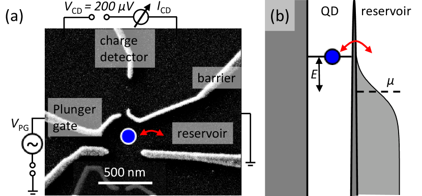
Figure 1: (a) Scanning electron micrograph of the device formed on a GaAs / AlGaAs heterostructure with a 2DEG 90 nm below the surface (dark grey area). Ti / Au gates (bright fingers) are patterned with e-beam lithography to capacitively deplete the 2DEG. The QD is formed in the place indicated by the blue circle and is tunnel coupled to a reservoir, as shown by the red arrow, while the other barrier is fully closed. An arbitrary waveform generator (AWG) is connected to the plunger gate to drive the QD. (b) An energy diagram indicates a tunneling process between the QD and the lead reservoir at energy $E$ measured from the Fermi energy $\mu$.

As a first experimental step we characterize the QD-reservoir system in thermodynamic equilibrium. A typical time trace of the charge detector current is shown in Fig. 2(a). In our experiment, we form a QD in a GaAs / AlGaAs two-dimensional electron gas (2DEG), as shown in Fig. 1. The confinement can be controlled by applying negative voltages to top-gates. The voltage $V_{\textnormal{PG}}$ applied to the plunger gate tunes the energy level $E$ linearly. The QD is coupled to a large contact region of the two-dimensional electron gas acting as the electron and heat reservoir characterized by the temperature $T\approx 40$ mK. We measure the tunnel rates for the last electron  Ciorga et al. (2000); Tarucha et al. (1996) with single-electron counting techniques, utilizing a nearby quantum point contact as a charge detector  Schleser et al. (2004); Vandersypen et al. (2004) and find electron tunneling at frequencies of the order of 100 Hz.

The occupation probability $\tilde{f}=\sum_{i=1}^{N}t_{\mathrm{in}}^{(i)}/\sum_{i=1}^{N}(t_{\mathrm{in}}^{(i)}+t_{\mathrm{out}}^{(i)})$ and tunneling rates $W_{\mathrm{in/out}}=N/\sum_{i=1}^{N}t_{\mathrm{in/out}}^{(i)}$, with the number of tunneling events $N$, are estimated from similar time traces taken at the indicated plunger gate energies Schleser et al. (2004); Vandersypen et al. (2004); Gustavsson et al. (2006) and presented in Fig. 2(b). The energy relaxation time for electrons injected from the QD into the Fermi sea is assumed to be much shorter than the time scales relevant for electron tunneling between the QD and the reservoir, and the chosen drive frequencies of less than $10$ Hz Fujisawa et al. (1998). Electron tunneling between the QD and the lead is described by Fermi’s golden rule, with energy independent tunnel coupling constants $\Gamma_{\textnormal{in}}$ and $\Gamma_{\textnormal{out}}$ and the Fermi distribution $f(E,T)$ describing the lead occupation at an energy $E$ measured from the Fermi energy of the lead, $\mu$. The resulting tunneling rates are

$$W_{\textnormal{in}}(E) =\Gamma_{\textnormal{in}}f(E,T)$$ (1a)

$$W_{\textnormal{out}}(E) =\Gamma_{\textnormal{out}}\left[1-f(E,T)\right].$$ (1b)

From a weighted least-mean-square fit of the measured tunnelling rates to Eqs. (1), the tunnel coupling constants, the position of the electrochemical potential, $\mu=0$, used as the zero-energy reference, as well as the temperature in units of plunger gate voltage of the lead are extracted. The fit is shown as solid blue line in Fig. 2(b). In the same figure, the solid green line is a least-mean-square fit of the estimated occupation probability $\tilde{f}$ to a second Fermi function, with the temperature and the resonance as fit parameters. From this fit, we recover the same temperature. However, we find that the occupation probability is one half around an energy value which is offset with respect to the Fermi energy by $E/kT=0.62\pm 0.08$.

From the partition function of the QD-reservoir system one can see that the offset of the energy where $\tilde{f}=1/2$ with respect to the Fermi energy is determined by $E=kT\ln(d)$ in the case where one electron is filled into an empty $d$-fold degenerate energy state. For the last electron, $d=2$ due to spin and hence, the occupation probability is one half at $E=kT\ln(2)$, as found in the experiment. At $E=\mu$, the probability for the energy level to be occupied is twice the probability for the state to be unoccupied. As shown in the inset of Fig. 2(b), the system obeys the detailed balance condition for the tunneling rates, $W_{\textnormal{in}}/W_{\textnormal{out}}=d\exp(-E/kT)$, with $d=2$, as found from the measured $d=\Gamma_{\textnormal{in}}/\Gamma_{\textnormal{out}}=1.97\pm 0.04$.

After having characterized the QD-lead system in equilibrium, our goal is to measure the equilibrium free energy change $\Delta F$ of the QD between an initial and a final state differing by a value $\Delta E\propto-V_{\textnormal{PG}}$ while it is driven out of equilibrium with respect to the reservoir by applying a time-dependent plunger gate voltage $V_{\textnormal{PG}}$. The Jarzynski equality Jarzynski (1997) provides the necessary tools for the theoretical description of such an experiment. It states that for an arbitrary drive protocol, the performed work $\Delta W$ during the drive satisfies

$$\langle\exp\left(-\frac{\Delta W}{kT}\right)\rangle=\exp\left(-\frac{\Delta F}{kT}\right),$$ (2)

where the average is taken over different repetitions of the drive protocol and $\Delta F$ is the equilibrium free energy change between the initial and final state of the drive. As the work can be evaluated for non-equilibrium situations, the Jarzynski equality allows to determine the equilibrium quantity $\Delta F$ with a non-equilibrium measurement.

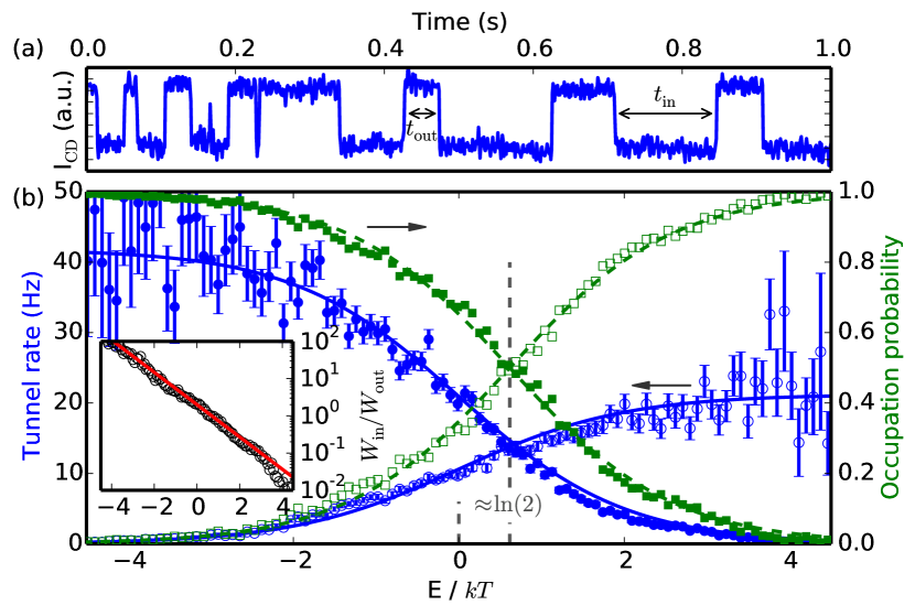
Figure 2: (a) A typical time trace of the charge detector current (I${}_{\textnormal{CD}}$). (b) Tunnel rates (filled blue for tunneling in and open blue dots for tunneling out) and relative frequency of occupation (green squares, filled for occupied and empty for non-occupied) extracted from CD time traces of 60 s. The abscissa is the negative plunger gate voltage measured from the Fermi energy and scaled by the temperature, $T=223\ \mu$V in units of $V_{\textnormal{PG}}$. The error bars indicate statistical errors assuming Gaussian fluctiations. The solid blue lines are weighted least-mean-square fits to Eq. (1), from which $\Gamma_{\textnormal{in}}=41.8\pm 1.6$ Hz and $\Gamma_{\textnormal{out}}=21.2\pm 0.6$ Hz and the temperature are determined. The dashed green lines are fits to Fermi functions centered around $\Delta E=k_{B}T\ln(2)$. Inset: The ratio of the two tunnel rates (black circles) is plotted as a function of energy from $\mu$, together with the exponential behaviour as expected from the detailed balance condition (red line).

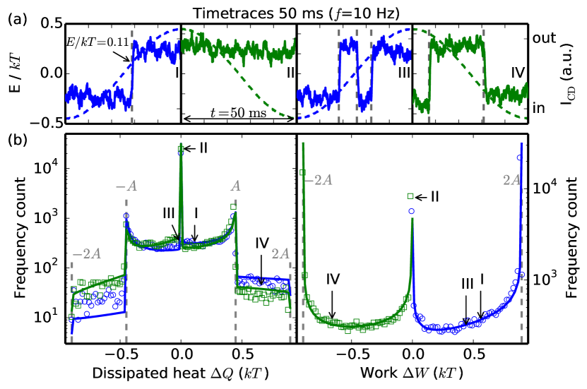
Figure 3: (a) Examples of drive realizations in upward (blue) and downward (green) direction, plotted as solid lines. The applied drive signals are shown as dashed lines. The driving is done by applying a voltage $V_{\textnormal{PG}}\propto-E$ to the plunger gate through an arbitrary waveform generator. From the position of the tunneling events (grey dashed lines) the heat and work of each realization are extracted. Bottom: The distribution for $\Delta Q$ (left) and $\Delta W$ (right) measured from approximately $20000$ realizations. Blue circles originate from upward and green squares from downward drive. The solid lines are rate equation calculations without free fitting parameters.

In our experiment, we apply a sinusoidal voltage ramp $V_{\textnormal{PG}}(t)$ to the plunger gate, which changes the energy of the electronic state in the QD from $E_{0}$ to $E_{1}$ and performs work on it as long as it is occupied [see Fig. 1(b)]. The drive protocol, as shown in the inset of Fig. 4, is characterized by the frequency $f$ and amplitude $A$ of the sinusoidal part of the protocol. Together, $A$ and $f$ determine the maximum steepness of the ramp and the initial ($E_{0}=-A$) and final ($E_{1}$) values of the QD energy level. We distinguish two drive directions, upward ($E_{1}>E_{0}$) and downward ($E_{0}>E_{1}$), and employ a waiting time of $\Delta t=0.5$ s for equlibration in-between. The respective initial and final states, $E_{0}^{(Up,Down)}$ and $E_{1}^{(Up,Down)}$, are indicated in the figure. Typical time-traces showing the charge-detector signal for four individual voltage ramps are shown in Fig. 3(a). In most cases, as shown on panel I, when the energy level of the QD starts well below the Fermi level and is raised above the Fermi level, the electron leaves the QD. If the drive frequency is large compared to the tunneling rates, realizations without tunneling events become probable, as shown in panel II. For each realization, we determine the work $\Delta W$ perfomed on the QD. When driving an occupied energy level of the QD, work is performed on the electron by the voltage source amounting to

$$\Delta W=\int_{E_{0}}^{E_{1}}n(E)dE,$$ (3)

where $n(E)\in\{0,1\}$ denotes the occupancy of the QD, which is directly measured by the charge detector signal. For example, in realization I, with the drive applied symmetrically around zero and $A=0.45\ kT$, the work performed on the electron in the QD is $\Delta W=(0.45+0.11)\ kT=0.56\ kT$. Note that the maximum amount of work that can be performed on or by the QD system is given by $\pm 2A$.

In addition, for each realization we determine the heat $\Delta Q$ dissipated in the contact from the energies $E_{i}$ of the QD state at which tunneling events occur. Each tunneling process contributes $\Delta Q_{i}=E_{i}$ for tunneling out and $\Delta Q_{i}=-E_{i}$ for tunneling into the QD. For example, in realization I, the electron tunnels at $0.11\ kT$ above $\mu$, hence $Q=0.11\ kT$ due to the relaxation of the electron in the lead. If more than one tunneling event occurs during a single realization, as shown in panels III and IV, the individual processes are added up,

$$\Delta Q=\sum_{i}\Delta Q_{i}=\sum_{i}E_{i}s_{i},$$ (4)

where $s_{i}$ distinguishes between tunneling-out processes, $s_{i}=1$, and tunneling-in processes, $s_{i}=-1$. The maximum amount of heat which can be dissipated in the lead during a single drive realization amounts to $\pm 2A$.

With the analysis described above, we now determine the relative frequency distributions of $\Delta W$ and $\Delta Q$ as shown in Fig. 3(b). The distributions for driving upwards are plotted as blue circles, while green squares are used for the distributions resulting from driving downwards. With the tunnel rates given in Fig. 2(b), $W_{\textnormal{in}}=42$ Hz and $W_{\textnormal{out}}=21$ Hz, and a drive frequency of $f=10$ Hz, realizations as shown in panel II of Fig. 3(b), i.e. without tunnel events and hence zero dissipated heat, are very probable, leading to a prominent delta-peak at $\Delta Q=0$ in Fig. 3(b). In these realizations, no work is done on the QD if the level stays empty during driving, leading to a peak at $\Delta W=0$ in Fig. 3(b). If it is occupied, the work equals plus or minus twice the drive amplitude for upward or downward drive direction, respectively. Hence, we observe two additional peaks, at $\Delta W=\pm 2A$, also corresponding to the single delta-peak at zero dissipation. From Fig. 3(b), it is apparent that the relative frequency for $|Q|\leq A$ is much higher than for $|Q|>A$. This is due to the fact that the maximum dissipation in a single realization depends on the occupancy of the initial and final state. For example, when driving an energy level downwards, the dissipated heat can only exceed $A$ if the state has been occupied in the beginning, as in realization IV. Contrary, $\Delta Q<A$ is only possible for downdrives if the final state is the less probable unoccupied state. Since the QD is thermally equilibrated by the waiting time before each drive, the occupancy of the initial state is given by the Fermi distribution and realizations with large $|Q|$ are suppressed. This effect, together with a comparably fast sinusoidal drive, also leads to the peaks found at $Q=\pm A$: they are mostly due to realizations starting in the more probable initial state and having a single tunnel event at the very end of the drive. Generally, the sharp features found in the probability distributions shown here are the signatures of non-equilibrium dynamics. For slower drives, the probability for intermediate dissipation $|Q|\sim 0$ increases and we find more Gaussian shaped distributions centered around zero dissipated heat (data not shown). This corresponds to the adiabatic limit, where a Gaussian shape with a width given by the fluctuation-dissipation theorem is expected  Nyquist (1928), as discussed in more detail in Ref.  Saira et al., 2012; Douarche et al., 2005 The detailed shape of the distributions depends on the relative amplitude $A/kT$ and frequency $f/\Gamma_{in,out}$ of the sinusoidal drive. For example, the distributions for work and dissipated heat are asymmetric with respect to the two drive directions because of the different rates for tunneling in and out of the QD, as discussed above. Using the standard rate equation approach  Saira et al. (2012) with parameter values extracted from the measurements of Fig. 2(b), we calculate the probability distributions for the work and the dissipated heat in each drive direction and find very good agreement with the experimental data.

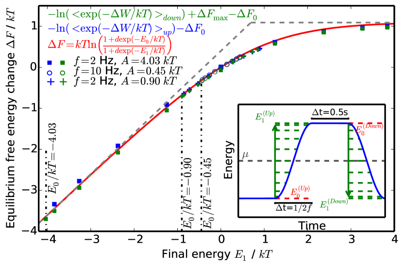
Figure 4: The free energy of the QD during the drive, obtained with non-equilibrium measurement, measured with respect to the Fermi energy. Experimental results are plotted in green for the downward and in blue for the upward drive direction. Different markers denote independent experiments with different drive parameters. The theory curve, Eq. 5, is plotted as solid red line, for $d=2$. Dashed grey lines indicate the expected linear increase at low $E_{1}$ as well as the saturation value for $E_{1}>E_{F}$. Inset: One full period of the drive is plotted in blue. A waiting time of 0.5 s ensures thermal equilibration of the initial state. Green dashed lines indicate the values of $E_{1}$ for which we extract $\Delta F$ from the experiment.

Utilizing Eq. (2), we now determine the equilibrium free energy change of the QD from the statistics of performed work. The prerequisite that the initial state must be thermally equilibrated Jarzynski (1997) is fulfilled by the waiting time. We determine the free energy change between the fixed initial and any freely chosen final state within the drive by analyzing $\Delta W$ as described above. As a result we get the free energy difference of the initial state and the chosen state within the drive. By varying the final state in the analysis, the change in free energy is determined along the full drive trajectory, as shown in Fig. 4. Different markers are used for the three measurements performed with the same gate configuration and QD resonance but with different values for $A$ and $f$, as indicated in the figure. Again, blue color denotes upward and green denotes downward drive direction. Each of the six drive protocols gives an independent estimate for $\Delta F$. From the extracted $\Delta W$ we also find that the average work $\langle W\rangle$ always exceeds the free energy change, as is expected for a system which is driven out of equilibrium.

Theoretically, the free energy is calculated from the difference of the partition sums of the initial ($i=0$) and final ($i=1$) states Reichl (1980),

$$\Delta F=kT\ln\left(\frac{Z_{0}}{Z_{1}}\right),\ Z_{i}=1+d\exp\left(\frac{-E_{i}}{kT}\right)$$ (5)

The theoretical curve is plotted as a solid red line in Fig. 4 for $d=2$, which is the value obtained from the equlibrium characterization above. Compatible with theory, we observe a linear increase of the free energy in the first part of the drive, where the electron is lifted to an energy level still well below the Fermi energy. The increase in $\Delta F$ slows down around the Fermi energy, as the probability of the QD to be occupied decreases. At energies well above the Fermi level, the occupation probability approaches zero and the free energy saturates. The six independent measurements of $\Delta F$ agree well with the theoretical value along the whole drive trajectory.

Small systematic deviations from the theoretical value of $\Delta F$ are found only for the data resulting from updrives at $f=2$ Hz and $A=4.03\ kT$. Experimental limitations are given by the stability of the sample as well as the bandwidth of the set up. The bandwidth limits the accuracy in the determination of the exact tunnel time in drive schemes where large amplitude and frequency are combined. These errors lead to uncertainties in $\Delta W$ and thereby also in $\Delta F$. The sample stability, on the other hand, sets a limitation to the number of repetitions which can be performed in a given configuration of the QD. Most importantly, the drive must be applied around the chosen operation point, equally for every repetition. Energy drifts in time therefore lead to systematic errors. Although we observe stable sample configurations over many hours, we implemented a feedback mechanism in order to align $E=0$ to the Fermi level $\mu$ every quarter hour. Offsets are taken into account in the analysis.

As demonstrated in Fig. 4, we have found good agreement between the experimental determination and theoretical expectation of the free energy change in our well-characterized system. This supports the idea that the free energy can be measured at any point of the drive in a system far out of equilibrium, independent of the drive parameters, by utilizing the Jarzynski equality. In the original work by C. Jarzinsky, an experimental test of equation 2 is suggested in a nanoscale system weakly coupled to a reservoir, where the fluctuation of the work is less then $kT$ and which evolves deterministically under its Hamiltonian  Jarzynski (1997). Even though the phase space evolution of the QD in our case is intrinsically non-deterministic due to tunneling events and the fluctuations are of the order of $kT$ drive amplitudes, we find Eq. 2 to be valid and the QD system to be a very suited testbed for the Jarzinsky equality.

As known from equilibrium thermodynamics, the free energy is a state variable and therefore independent of the trajectory. When the system is driven out of equilibrium, such trajectory-independent quantities are not generally available and the situation becomes more complex. In this work we have shown that an equilibrium quantity, the free energy of a two-fold degenerate single electron state, can be measured with an experiment driving the system far from equilibrium. Our results show that thermodynamic quantities such as work and dissipation can be understood on the level of individual quantum states and in nonequilibrium. The good agreement with theoretical calculations proves that the simple system we have used suits well for studying more complex phenomena out of equilibrium. As a direct consequence of the presented work, we expect the relation between thermodynamics and information theory as well as influences of dissipation on future fast drives of qubits to be studied in quantum dot systems.