On the Optimality of Square Root Measurements in Quantum State Discrimination
Abstract
Distinguishing assigned quantum states with assigned probabilities via quantum measurements is a crucial problem for the transmission of classical information through quantum channels. Measurement operators maximizing the probability of correct discrimination have been characterized by Helstrom, Holevo and Yuen since 1970’s. On the other hand, closed–form solutions are available only for particular situations enjoying high degrees of symmetry. As a suboptimal solution to the problem, measurement operators, directly determined from states and probabilities and known as square root measurements (SRM), were introduced by Hausladen and Wootters. These operators were also recognized to be optimal for pure states equipped with geometrical uniform symmetry (GUS). In this paper we discuss the optimality of the SRM and find necessary and sufficient conditions in order that SRM maximize the correct decision probabilities for set of states formed by several constellations of GUS states. The results are applied to some specific examples concerning double constellations of quantum phase shift keying (PSK) and pulse position modulation (PPM) states, with possible applications to practical systems of quantum communications.
pacs:
03.67.HkI Introduction
The long standing problem of transmitting classical information through a noiseless quantum channel refers to the following scenario. A classical information source emits a symbol in a finite alphabet, say , whose nature is irrelevant to the problem. The symbols are emitted with probabilities satisfying the properties and . On the basis of the symbol emitted by the classical source, the transmitter (conventionally known as Alice) prepares the quantum channel in a state belonging to a set of agreed quantum states, generally mixed states with density operators which are semidefinite positive () and have unitary trace (). The quantum ensemble can be conveniently represented by the weighted density operators .
The problem of the receiver (conventionally known as Bob) is to extract as well as he can classical information from the quantum channel he and Alice share. In this task Bob is assumed to know both the quantum states and their probabilities . We assume that the measurement and decision strategy of Bob is the quantum hypothesis testing introduced by Helstrom Helstrom (1976). The strategy consists in performing on the quantum channel a positive operator–valued measurement (POVM) with measurement operators semidefinite positive () and resolving the identity operator, namely, . The conditional probability that the measurement gives the result provided that the state is turns out to be . The usual task of Bob is the choice of the POVM maximizing the probability of correct decision
| (1) |
The problem solution is given by well known general results due to Holevo Holevo (1973), Yuen et al. Yuen et al. (1975), and Helstrom Helstrom (1976) (see also Barnett and Croke (2009), and Konig et al. (2009) for a connection with min–entropy of a classical source) and is summarized by the following theorem.
Theorem 1. The measurement operators give the maximum correct detection probability if and only if the operator
| (2) |
satisfies the conditions
| (3) |
for each . The above condition implies also that is semidefinite positive and that the equalities
| (4) |
hold true for all .
Unfortunately, closed form solutions are available only in few very particular cases, generally implying pure states enjoying high degrees of symmetry. Indeed, as pointed out in Eldar et al. (2003), serious mathematical difficulties arise because of the non linearity of the problem, which turns out to be a convex semidefinite programming problem.
If the states prepared by Alice are pure, namely, , it can be shown Belavkin (1975) that also the measurement operators have rank 1, namely, . Then the correct detection probability (1) depends on the inner products of the states and of the measurement vectors , namely,
| (5) |
where are the weighted states. The optimization problem reduces to find the measurement vectors maximizing the correct detection probability (5). In accordance with the general case, the vectors must resolve the identity operator of the Hilbert space spanned by the states
| (6) |
In the following we assume that the weighted states are linearly independent. This is not at all too restrictive for all situations of practical interest. In this case it can be shown Kennedy (1973) that the optimal measurement vectors (to be determined) form an orthonormal basis. Since the weighted states are linear combinations of the measurement vectors, provided that the states are collected into a matrix and the measurement vectors into a matrix , i.e.,
| (7) |
a matrix relation holds. The entries of the matrix are given by . The joint input–output probabilities become and the corresponding correct decision probability turns out to be
| (8) |
The optimization problem can be conveniently formulated introducing the Gram matrix of the weighted states , namely . Then, using (6) gives
| (9) |
and in matrix form. In conclusion, the optimal detection problem reduces to find the factorization of the Gram matrix that maximizes probability (8). Provided that is the result of the optimization, the measurement vectors are obtained by . Note that the independence of the states implies that the Gram matrix is positive definite, so that is invertible. Unfortunately the factorization (9) of the Gram matrix leads to a set of quadratic equations, which can be solved only by numerical programs, at least in general.
A different approach is based on a very popular suboptimal measurement, known as square root measurement (SRM), which was introduced by Hausladen and Wootters Hausladen and Wootters (1994) and thoroughly discussed by Eldar and Forney Eldar and Forney (2001). In the framework discussed above, the square root measurement corresponds to the factorization of the Gram matrix with square root of the Gram matrix itself. Under our assumptions both the matrix and its inverse are definite positive. The matrix of the measurement vectors is given by and the correct detection probability is the sum of the squares of the diagonal entries of , i.e.,
| (10) |
Even though this measurement is not optimal in general, it exhibits interesting properties. It can be straightforwardly obtained by the Gram matrix and gives performances near to the optimum provided that the weighted states are almost orthogonal. Indeed Hausladen et al. Hausladen et al. (1996) have shown that SRM (also known as ”pretty good” measurement) is asymptotically optimal, in the sense that it is good enough to be used as non local measurement in the proof of their fundamental theorem on the classical capacity of a quantum channel. More recently SRM has found application Bacon et al. (2005); Moore and Russell (2007); Hayashi et al. (2008) in the search of optimal measurement for distinguishing hidden subgroup states, providing an interesting approach to the large class of quantum computational problems linked to the hidden subgroup problem. In any case SRM furnishes a lower bound to the optimal performance and it may be assumed as a starting point to find the optimal measurement through unitary transformations.
The SRM turns out to be the optimal measurement when the states exhibit a high degree of symmetry. Then, particular attention has been given to applications of the SRM to states enjoying geometrically uniform simmetry (GUS), i.e., sets of states that are invariant with respect to a unitary transformation Ban et al. (1997); Eldar and Forney (2001). This is particularly interesting for practical quantum communication systems using quantum phase shift– keying (QPSK) Kato et al. (1999) and pulse position modulation (PPM) Cariolaro and Pierobon (2010a). Also extensions to mixed state have been considered Eldar et al. (2004); Cariolaro and Pierobon (2010b).
The aim of the present paper is to show that the optimal feature of SRM is by no means confined to states enjoying GUS and having equal probabilities. In particular we consider a set of states composed by distinct constellations of states enjoying the same GUS (we use the term “constellation” borrowed from the telecommunications jargon for the more general “subset”). This is a particular case of the compound geometrical uniform symmetry discussed in Eldar et al. (2004). The novelty of our approach stays in the fact that we find necessary and sufficient conditions in order that SRM is the optimal measurement for this case. Moreover we present possible applications to practical quantum communication systems as PSK and suggest a version of PPM improving its efficiency.
The paper is organized as follows. In Section II we revisit two important results concerning our topic. The first, due to Helstrom Helstrom (1982), characterizes the factorization that maximixes the correct decision probability. The second, due to Sasaki et al. Sasaki et al. (1998), gives simple sufficient conditions guaranteeing that the SRM is the optimal measurement. In particular the last result enables one to show in a very simple way that SRM is optimal for states enjoying geometrical uniform symmetry. The main result of the paper is presented in Section III, where a necessary and sufficient condition is furnished in order that the SRM is optimal for a set formed by constellations of GUS states generated by the same unitary transformation but applied to different states. In Section IV the result is applied to a double constellation of quantum PSK states, showing that SRM may be optimal also for states with non uniform probabilities. In Section V we consider a double constellation of PPM states and show that the SRM is optimal for this case and leads to a communications scheme more efficient than the original PPM. Some conclusions close the paper.
II The SRM as optimal measurement
While Theorem 1 refers to the general case of mixed states, a simple characterization of the optimal measurement for independent pure states is given by the following theorem.
Theorem 2. The factorization maximizes the correct decision probability if and only if the following conditions hold:
i) for each and
| (11) |
The theorem, not frequently cited in the literature, has been proved by Helstrom in a paper Helstrom (1982) concerning an iterative search of the optimal measurement. The proof of the theorem, given in appendix of the paper, is somewhat intricate. A simplified version of the proof is given here in Appendix A.
As we pointed out, the SRM corresponding to the factorization with is not optimal in general. On the basis of the Theorem 2, Sasaki et al. Sasaki et al. (1998) in a paper about the superadditivity of the capacity of a quantum channel have found a nice sufficient condition for the optimality of SRM. The following theorem gives a generalization of the result.
Theorem 3. Assume that the Gram matrix (and its square root ) is block diagonal, namely, . Then, the square root measurement is optimal if and only if the square root of each block has equal diagonal entries.
Proof. If the matrix is formed by a single block, it is irreducible and its associated directed graph is strongly connected Horn and Johnson (1990). Then, the indexes may be ordered into a cycle such that for each . Since is Hermitian, and condition (11) is satisfied if and only if for each or, equivalently, if the diagonal entries of have a common value . Therefore, condition (12) of Theorem 2 holds in that is positive definite. If has many diagonal block, the proof can be applied to each block.
Confining our attention to the case of a single block, since , the theorem is equivalent to say that the SRM is optimal if and only if the probabilities of correct decision is , independent of the state transmitted. In particular, the optimal correct decision probability turns out to be
| (14) |
It is worthwhile to note that the optimality of the SRM depends only on the Gram matrix. Since this is invariant with respect to unitary transformations, if a constellation of weighted states satisfy the conditions of Theorem 3, any other constellation obtained via a unitary transformation admits optimal SRM with the same error probability. Of course the optimal SRM operators vary according to the unitary transformation.
The most known case of optimality of the SRM concerns states equipped with geometrical uniform symmetry (GUS) Ban et al. (1997); Eldar and Forney (2001). The weighted states enjoy GUS if , , where is a unitary operator satisfying the condition . This generalizes the usual definition of GUS states as satisfying the condition , and having equal probabilities . The proof of the optimality of the SRM is an immediate consequence of Theorem 3. Indeed, the entries of the weighted Gram matrix become
| (15) |
and depend only by . One concludes that the matrix is circulant Davis (1979). (Details on the basic properties of circulant matrices are collected for convenience in Appendix B). Then has spectral decomposition
| (16) |
(see (61)) where is the unitary Fourier matrix (62) and the diagonal matrix collects the (positive) eigenvalues of . Then
| (17) |
is circulant, its diagonal entries are equal, and the SRM is optimal. In particular
| (18) |
and
| (19) |
The GUS is by no means the only case where Theorem 3 finds application. As an elementary example consider the Gram matrix
| (20) |
of two states and with equal probability and . Note that this matrix is not circulant in general. Its square root matrix is
| (21) |
with and . By virtue of Theorem 3 the SRM is optimal. A simple algebra shows that
| (22) |
so that the Helstrom bound
| (23) |
holds. This is perhaps the simplest proof of the Helstrom bound, at least for equilikely states. In the literature the SRM is usually presented in connection with GUS states having equal probabilities. However, the extension to other situations is possible (see Mochon (2006) for a detailed, but scarcely constructive, theoretical analysis). Recently Kato Kato (2013) has found a closed form expression of the input probabilities for which the measurement operators obtained from the not weighted Gram matrix are optimal in the case of three coherent states , and .
III Multiple constellations of GUS states
Here we consider a collection of states , , , defined as
| (24) |
where is a unitary operator such that . In other words the set of states is formed by constellations of GUS states obtained by the same unitary operator , starting from different states . Moreover we relax the hypothesis of equal probabilities, only assuming that the states of each constellation have the same probability, namely, with . Under these assumptions we find a sufficient and necessary condition for the optimality of the SRM. This is a particularization of the concept of compound geometrical uniform (CGU) states, introduced by Eldar et al. Eldar et al. (2004), where and the unitary operators form a (not necessarily Abelian) multiplicative group.
We begin by ordering the states as
| (25) |
The weighted Gram matrix of the states may be partitioned in the form
| (26) |
where the submatrices have order and entries
It follows that the matrices are circulant and are simultaneously diagonalizable as , where is the Fourier matrix defined in Appendix B. Then , with and the blocks of
| (27) |
are diagonal matrices of order .
The square root of , say , has the same structure as . Indeed, by a joint permutation of rows and columns generated by a permutation matrix the matrix can be transformed into a block diagonal matrix
| (28) |
Incidentally, the permutation converting the ordering (25) of the states into the ordering
| (29) |
is the natural choice. Since the matrix is positive definite as , also and its diagonal blocks are positive definite. Then
| (30) |
is well defined. Applying to the inverse permutation one gets , where
| (31) |
where the blocks are diagonal matrices of order .
The diagonal blocks of the square root of the weighted Gram matrix are . This results in a circulant matrix with diagonal elements, say , depending on . The condition of optimality of the SRM (see Theorem 3) is satisfied if and only if is independent of . This is summarized by the following theorem.
Theorem 4. The SRM is optimal for the multiple constellation of GUS states if and only if the diagonal blocks of the square root of the weighted Gram matrix have equal diagonal entries.
An alternative criterion derives from the fact that
| (32) |
Then the condition of optimality of the SRM is satisfied if and only if the blocks have equal traces.
Finally, provided that the SRM is optimal, the correct decision probability becomes
| (33) |
IV Double quantum PSK constellation
As a first application of the above theory we consider a double quantum binary phase shift keying (BPSK) with four coherent states and in a Fock space. The system is a particular case of the scheme discussed in the previous section by setting
| (34) |
In this case the symmetry operator is the rotation operator with and annihilation and creation operators in the Fock space giving . According to our previous assumption the probabilities of and are and respectively, with .
The Gram matrix depends on the inner products
| (35) |
The blocks of the weighted Gram matrix turn out to be
| (36) | |||
| (37) |
Applying the discrete Fourier transform (63) gives the eigenvalues of the block
| (38) |
Similarly, the eigenvalues of are
| (39) |
and the eigenvalues of
| (40) |
The weighted Gram matrix is decomposed as , where is the matrix (27) with diagonal blocks , and .
The square root can be evaluated taking advantage of the sparsity of the matrix , or, as an alternative, considering the permutation that converts the ordering of the states into (29). The result is the block-diagonal matrix (28), which is related to through , and has diagonal blocks
| (41) | |||
| (42) |
The square root has the same structure of , and can be evaluated from the square root of and , with
| (43) |
where . Similarly the square root of , which can also be obtained from (43) with the substitutions
| (44) |
Finally, the square root is obtained applying the inverse permutation to the block-diagonal matrix . The blocks of are still diagonal, and in particular
| (45) |
and
| (46) |
with obtained from with the substitutions (44). The square root of the weighted Gram matrix is then obtained through the Fourier transform, .
The optimality of SRM can be verified with the aid of Theorem 4, or, as an alternative, through the conditions (32). Given a set of parameters and , the optimality is not assured. However, it is worthwhile to investigate how one of the parameters should be optimized given the others, in order to meet the optimality conditions. This is the topic of this section, where we investigate the optimization of the variable given the parameters . Although this optimization can be (numerically) performed for arbitrary , we focus our attention on two particular cases.
IV.1 Case
As a first case, we consider . Practical application of this case arises when the transmitter, supposed to produce a Quaternary-PSK, has a misalignment or a systematic bias error in the angle defining one of the two constellations. Without loss of generality, the alphabet can be defined with two real parameters, and , with defining the angular shift between the two binary constellations.
The entries in the weighted Gram matrix simplifies, and the inner products between the states become
It is immediate to verify that with these positions, condition (32) for the optimality of the SRM is satisfied by . That is, the equal prior probability between the symbols gives the optimality of SRM, even in the case .
In Fig. 1 the performances of the Double BPSK are plotted as a function of the mean photon number employed in each transmitted state. In the figure, different curves correspond to the values of the phase shift . As we can see, the lines are monotonically increasing in both the value of and . In addition, the performances are similar when is around , which is the situation of the Quaternary PSK, while they drop quickly for lower values of the phase shift.

IV.2 Case
As a second case of study, we consider . This set of constellations corresponds to the modulation scheme known as 4-Pulse Amplitude Modulation (PAM). While usually an equal prior probability is assumed for the transmitted states, here we study the optimization of this probability such that the SRM are optimal.
The inner products between the states read
Again, we resort to conditions (32) in order to find the value of that makes the SRM optimal. In this case, there are no evident solutions, and the authors could not find any closed form solution, so we turn to numerical algorithms to find the optimal value.

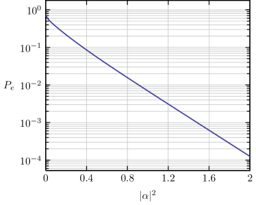
The results of the numerical optimization are plotted in Fig. 2, as a function of the mean photon number of the states . Note that while for low values of the prior moves away from equal distribution, the optimal solution tends to as the value of increases. The corresponding performance is plotted in Fig. 3, which show an increase in the performance as the value of increases.
We have compared the performance of the SRM with optimal a priori probabilities with the performances of both the SRM and the optimal measurement (evaluated via semidefinite programming Eldar et al. (2003)) with equal a priori probabilities. The results are practically indistinguishible if plotted as in Fig. 3. This further comfirms that SRM is really a very good measurement in cases of practical interest. In particular, in the present case, optimizing the a priori probabilities does not reduces in significant way the error probability.
V Double quantum PPM constellation
V.1 Simple quantum PPM constellation
A popular scheme proposed for deep space quantum communications is the pulse position modulation (PPM) Dolinar et al. (2006). This scheme can be modeled in a Hilbert space formed by replicas of the Fock space . The states used by Alice are tensor products
| (47) |
where only coincides with a coherent state , while the other coincide with the null state . For instance, for , the states are
| (48) | |||
In practical realizations, in correspondence with the symbol the laser radiates only in the –th slot of a time frame of slots.
Although the symmetry of the states is apparent (every state is a cyclic permutation of the preceding), the evaluation of the unitary symmetry operator in the tensor space is by no means trivial Cariolaro and Pierobon (2010a). In any case, provided that the states have equal probabilities , the weighted Gram matrix is given by
| (49) |
with (without loss of generality is assumed real). Since is circulant as , the SRM is optimal. Applying the discrete Fourier transform (B5) gives the eigenvalues of
| (50) | |||
Applying to the eigenvalues of the inverse discrete Fourier transform (B6), one gets the first row of , namely,
Note that has the same structure of with equal entries out of the diagonal.
The correct detection probability is obtained by (19) and is
V.2 Double quantum PPM constellation
Here we propose a new PPM scheme with the goal of doubling the number of the states and, possibly, of improving the capacity of the quantum communication system. We consider a double constellation in
where, as in the ordinary quantum PPM, includes only one non null state in the –th slot, while includes only one non null state in the –th slot. To maintain the symmetry of the problem, we assume that the states have equal probability . The weighted Gram matrix turns out to to be
where and . Simple considerations lead to the following circulant matrices
The discrete Fourier transform (63) gives the eigenvalues of
| (51) | |||
and the eigenvalues of
| (52) | |||
Then with
| (53) |
where and . It follows that
| (54) |
where the diagonal matrices and satisfy the conditions and . Since the diagonal blocks of coincide, the SRM is optimal. Simple computations lead to and with
Finally, using the inverse discrete transform (64), we get the first rows of the circulant matrices and
Note that and have equal entries out of the diagonal as a consequence of the particular symmetry.
Finally (33) gives the correct decision probability of the double PPM
V.3 Mutual information comparison
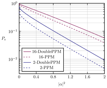
In Fig. 4 the error probabilities of the simple and double PPM are compared for and in terms of the mean number of photons per symbol related to the parameter by . The error probability of double PPM is larger, but its states are twice as many. Then a significant comparison requires the evaluation of the informations transferred by the systems.
The channel defined by the simple PPM is a symmetric channel with joint input–output probabilities and for . The marginal probabilities are uniform . Then the mutual information turns out to be
| (55) | ||||
The channel defined by the double PPM has joint input–output probabilities , , , while the other crossover probabilities have common value . The marginal probabilities are uniform as a consequence of the symmetry. In conclusion the mutual information turns out to be
| (56) |
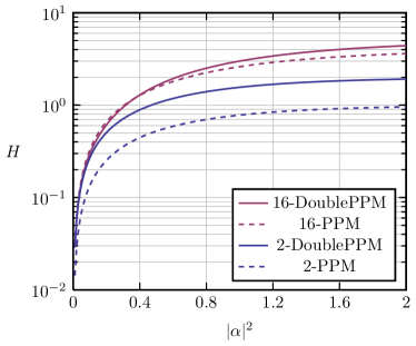
Asymptotically, as increases (and tends to zero), tends to and tends to with a gain of one bit per symbol. The mutual informations and , coinciding with the capacities of the channels, are compared in Fig. 5 for and .
Two remarks are adequate. First, the double PPM scheme is a combination of the simple PPM scheme and of a binary PSK scheme. Further gain could be obtained combining PPM with –PSK, using PPM constellation with non empty states , . Second, from a practical point of view, double PPM implies some complications, both on the transmitter and on receiver side. At the transmitter the on–off modulation must be replaced by a phase modulation, while at the receiver a simple photon counter must be replaced by a phase sensitive device. We do not insist on these topics that are beyond the scope of the paper.
VI Conclusions
The square root measurement furnishes an alternative approach to the reliable discrimination of quantum states. This measurement is only suboptimal, in general, but it is well known that it turns to be optimal for quantum states enjoying geometrically uniform simmetry. In this paper, we showed that the square root measurement is optimal also in other situations of practical interest. In particular we found necessary and sufficient conditions for the optimality in the presence of multiple constellations of symmetrical states also with non uniform probabilities. As an application example we considered the case of two pairs of quantum binary symmetrical states (PSK states). Finally, the theory is applied to a possible improvement of the pulse position modulation (PPM) scheme that increases the capacity of the resulting channel.
Acknowledgements.
Nicola Dalla Pozza acknowledges partial support by the ‘Borsa Gini’ scholarship, awarded by ‘Fondazione Aldo Gini’, Padova, Italy.Appendix A Proof of Theorem 2
We apply the Theorem 1 to the operators and and preliminarily note the following matrix representations of , and in terms of the orthonormal basis :
| (57) |
If the measurement is optimal statement i) follows directly from (4) and is semidefinite positive. Since is not singular, it remains to prove that the diagonal entries of (of ) are different from 0. Assume that . Then, it must exist such that , for otherwise all the states would be orthogonal to against the assumption of their linear independence. Without loss of generality, assume that . As a consequence of i) we have also . Now, if we change the roles of the measurement vectors and , the matrix is modified in , with for , , and . Denoted by the new correct decision probability, we get contradicting the optimality of . One concludes that has non zero diagonal entries and is definite positive. In order to prove the sufficiency note that the matrices are Hermitian and . Then they satisfy the conditions of a theorem on the eigenvalues of Hermitian matrices (Horn and Johnson, 1990, Theorem 4.3.4) which states that, denoted by the eigenvalues of and by the eigenvalues of arranged in increasing order, we have
| (58) |
If is positive definite, it follows that . Since in the –th column vanishes, at least one of its eigenvalues vanishes and . One concludes that all eigenvalue of are non negative and is semidefinite positive. Since this holds true for each , the condition (4) of Theorem 1 is satisfied and the operators provide the optimal measurement.
Appendix B Circulant matrices
We collect in this appendix for convenience some properties of the circulant matrices which are used in the paper. For more details the reader is deferred to the literature on the topic, for instance Davis (1979).
A matrix of order is said circulant if
| (59) |
i.e., if
| (60) |
In other words is circulant if its rows are cyclic permutation of the first row. A matrix is circulant if and only if has spectral decomposition
| (61) |
where is the (unitary) Fourier matrix with entries
| (62) |
and the diagonal matrix collects the eigenvalues of . The circulant matrices of order form a multiplicative commutative group of matrices simultaneously diagonalizable. The eigenvalues of the circulant matrix can be obtained from the first row of the matrix via the discrete Fourier transform
| (63) |
Finally, the inverse discrete Fourier transform gives the first row of
| (64) |
References
- Helstrom (1976) C. W. Helstrom, Quantum Detection and Estimation Theory (Academic Press, New York, 1976).
- Holevo (1973) A. Holevo, Journal of Multivariate Analysis 3, 337 (1973).
- Yuen et al. (1975) H. P. Yuen, R. S. Kennedy, and M. Lax, IEEE Transactions on Information Theory 21, 125 (1975).
- Barnett and Croke (2009) S. M. Barnett and S. Croke, Journal of Physics A: Mathematical and Theoretical 42, 062001 (2009).
- Konig et al. (2009) R. Konig, R. Renner, and C. Schaffner, IEEE Transactions on Information Theory 55, 4337 (2009).
- Eldar et al. (2003) Y. Eldar, A. Megretski, and G. Verghese, IEEE Transactions on Information Theory 49, 1007 (2003).
- Belavkin (1975) V. P. Belavkin, Stochastics 1, 315 (1975).
- Kennedy (1973) R. S. Kennedy, Research Laboratory of Electronics, MIT Quarterly Progress Report No. 110 pp. 142–146 (1973).
- Hausladen and Wootters (1994) P. Hausladen and W. K. Wootters, Journal of Modern Optics 41, 2385 (1994).
- Eldar and Forney (2001) Y. C. Eldar and G. D. J. Forney, IEEE Transactions on Information Theory 47, 858 (2001).
- Hausladen et al. (1996) P. Hausladen, R. Jozsa, B. Schumacher, M. Westmoreland, and W. K. Wootters, Physical Review A 54, 1869 (1996).
- Bacon et al. (2005) D. Bacon, A. Childs, and W. van Dam, in 46th Annual IEEE Symposium on Foundations of Computer Science (FOCS’05) (IEEE, 2005), pp. 469–478.
- Moore and Russell (2007) C. Moore and A. Russell, Quantum Information & Computation 7, 752 (2007).
- Hayashi et al. (2008) M. Hayashi, A. Kawachi, and H. Kobayashi, Quantum Information & Computation 8, 345 (2008).
- Ban et al. (1997) M. Ban, K. Kurokawa, R. Momose, and O. Hirota, International Journal of Theoretical Physics 36, 1269 (1997).
- Kato et al. (1999) K. Kato, M. Osaki, M. Sasaki, and O. Hirota, IEEE Transactions on Communications 47, 248 (1999).
- Cariolaro and Pierobon (2010a) G. Cariolaro and G. Pierobon, IEEE Transactions on Communications 58, 1213 (2010a).
- Eldar et al. (2004) Y. C. Eldar, A. Megretski, and G. Verghese, IEEE Transactions on Information Theory 50, 1198 (2004).
- Cariolaro and Pierobon (2010b) G. Cariolaro and G. Pierobon, IEEE Transactions on Communications 58, 623 (2010b).
- Helstrom (1982) C. Helstrom, IEEE Transactions on Information Theory 28, 359 (1982).
- Sasaki et al. (1998) M. Sasaki, K. Kato, M. Izutsu, and O. Hirota, Physical Review A 58, 146 (1998).
- Horn and Johnson (1990) R. A. Horn and C. R. Johnson, Matrix Analysis (Cambridge University Press, New York, 1990).
- Davis (1979) P. J. Davis, Circulant Matrices: Second Edition, AMS Chelsea Publishing (Wiley, New York, 1979).
- Mochon (2006) C. Mochon, Phys. Rev. A 73, 032328 (2006).
- Kato (2013) K. Kato, Tamagawa University Quantum ICT Research Institute Bulletin 3, 29 (2013).
- Dolinar et al. (2006) S. Dolinar, J. Hamkins, B. Moision, and V. Vilnrotter, in Deep Space Optical Communications, edited by H. Hemmati (Wiley, Hoboken, New Jersey, 2006), chap. 4.