Self-gravity, resonances and orbital diffusion in stellar discs

Abstract

Fluctuations in a stellar system’s gravitational field cause the orbits of stars to evolve. The resulting evolution of the system can be computed with the orbit-averaged Fokker-Planck equation once the diffusion tensor is known. We present the formalism that enables one to compute the diffusion tensor from a given source of noise in the gravitational field when the system’s dynamical response to that noise is included. In the case of a cool stellar disc we are able to reduce the computation of the diffusion tensor to a one-dimensional integral. We implement this formula for a tapered Mestel disc that is exposed to shot noise and find that we are able to explain analytically the principal features of a numerical simulation of such a disc. In particular the formation of narrow ridges of enhanced density in action space is recovered. As the disc’s value of Toomre’s $Q$ is reduced and the disc becomes more responsive, there is a transition from a regime of heating in the inner regions of the disc through the inner Lindblad resonance to one of radial migration of near-circular orbits via the corotation resonance in the intermediate regions of the disc. The formalism developed here provides the ideal framework in which to study the long-term evolution of all kinds of stellar discs.

1. Introduction

Many, perhaps all, stars are born in a stellar disc. Major mergers destroyed some discs quite early in the history of the Universe, but many others have survived to the present day, including the disc of which the Sun is a part. Hence an understanding of the dynamics and evolution of stellar discs is an essential ingredient of cosmology. Conversely, cosmology provides the framework within which disc dynamics should be studied because dark-matter halos make large contributions to the gravitational fields in which discs move, and dark-matter substructures are major contributors to the gravitational noise to which discs are exposed.

Serious study of disc dynamics got underway in the 1960s with seminal works by Lin, Shu, Goldreich, Toomre and Lynden-Bell. Although some important insights were gained at that stage, fundamental questions were left open. While the earliest work was almost entirely analytic in nature, numerical simulations of stellar discs became more important over time, and revealed important aspects of disc dynamics that were hard to understand analytically. In particular it emerged that discs that are completely stable at a linear level nevertheless develop spiral structure that eventually grows to amplitudes of order unity, so the disc becomes something like a barred spiral galaxy (Sellwood, 2012, hereafter S12). Sellwood & Carlberg (2014) recently offered a convincing explanation of this phenomenon that hinges on the fact that resonances localise the impact that a fluctuation has on a disc. This localisation is the major focus of this paper.

Self-gravitating discs are responsive dynamical systems, in which (a) rotation provides an abundant supply of free energy, and (b) resonances play a key role. The ready availability of free energy leads to some stimuli being powerfully amplified, while resonances localise the dissipation of free energy with the result that even a very small stimulus can result in a disc evolving to an equilibrium that is materially different from the one from which it started.

The stimuli to which discs respond are various sources of gravitational noise. They include, Poisson noise arising from the finite number of stars in a disc, Poisson noise arising from the finite number of giant molecular clouds in the interstellar medium, and Poisson noise arising from the finite number of massive sub-halos around a galaxy. Spiral arms in the distribution of gas provide another source of gravitational noise, while the rotating gravitational field of a central bar constitutes a source of stimulus that is more systematic than noisy. The history of a real stellar disc will largely comprise responses to all these stimuli.

In the solar neighbourhood at least three distinct manifestations of such responses are evident:

• The random velocity of each coeval cohort of stars increases with the cohort’s age (Wielen, 1977; Aumer & Binney, 2009).

• The velocity distribution at the Sun contains several “streams” of stars (Dehnen, 1998). Each such stream contains stars of various ages and chemistries that are all responding to some stimulus in a similar way (Famaey et al., 2005).

• In the two-dimensional space in which one coordinate is angular momentum $J_{\phi}$ and the other is a measure of a star’s radial excursions, such as the radial action $J_{r}$, the density of stars shows elongated features. The density of stars is depressed near $J_{r}=0$ but enhanced at larger $J_{r}$ in such a way that the whole region of disturbed stellar density forms a curve that is consistent with being a curve on which a resonant condition such as $2\Omega_{\phi}-\Omega_{r}=\hbox{constant}$ holds (Sellwood, 2010; McMillan, 2013). We shall call a feature of this type a resonance ridge. Sellwood & Carlberg (2014) have argued that resonance ridges play a crucial role in the long-term dynamics of stellar discs.

Numerical simulations of stellar discs are extremely challenging because the near two-dimensional geometry of discs combined with their responsive nature causes discreteness noise to be dynamically important unless the number of particles employed exceeds $\sim 200\,000$. Hence only recently has it become straightforward to simulate a disc with a sufficient number of particles for discreteness noise to be dynamically unimportant for many dynamical times (S12). It is particularly hard to simulate accurately a disc that is embedded in a cosmological simulation and thus exposed to cosmic noise. Moreover, the utility of a simulation is greatly increased if one understands analytically why it evolves the way it does. A goal of this paper is to show the extent to which perturbation theory explains a phenomenon – resonance ridges – that is seen in both numerical simulations and surveys of the solar neighbourhood.

Perturbation theory is much more than a device for computing approximate solutions to equations: throughout physics it provides the conceptual framework we use to understand phenomena. Examples include the concepts of a free particle and an interaction in particle physics, a phonon and a gravity wave in condensed-matter physics, semi-major axis and eccentricity in planetary dynamics, and so on. The natural way to increase our understanding of the dynamics of stellar discs is to practise the application of perturbation theory to these systems, so we may gain insight into how these fascinating systems work, and learn how one can think about them most profitably.

Kalnajs (1971) laid the foundations of perturbation theory for stellar discs. The theory is based on the use of angle-action coordinates – the coordinates that were introduced to understand the dynamics of the solar system. These coordinates are being increasingly used to build equilibrium models of hot and cold stellar systems (Binney, 2010, 2014; Piffl et al., 2014), and to study the dynamics of star streams (Helmi & White, 1999; Sellwood, 2010; McMillan, 2013; Eyre & Binney, 2011; Sanders & Binney, 2013). Binney & Lacey (1988) used these coordinates to derive the orbit-averaged Fokker-Planck equation for a stellar disc. However, they did not consider the origin of the fluctuations in the gravitational potential that drive stellar diffusion. Weinberg (2001a) divided the driving fluctuations into the contribution from some external stimulus, and the self-consistent dynamical response of the system itself to the stimulus. Weinberg’s treatment was adapted to systems that are spherical when unperturbed, while here we restrict ourselves to razor-thin discs, in which case the construction of the angle-action coordinates is trivial.

The paper is organised as follows. Section 2 recalls from Binney & Lacey (1988) and Weinberg (2001a) the general principles of secular evolution, the orbit-averaged Fokker-Planck equation, and the use of a set of biorthonormal potential-density pairs to compute the diffusion tensor that is jointly generated by an external stimulus and the system’s response to this stimulus. Section 3 specialises this formalism to a razor-thin, cool disc by introducing a set of basis functions that comprise localised, tightly-wound spirals. Using these basis functions we are able to reduce the computation of the diffusion tensor, which in principle requires a double sum over basis functions, to a single integral over radial wavenumbers. In Section 4 we compute the diffusion tensor for a tapered Mestel disc that is excited by shot noise, and show that the resulting predictions for the disc’s evolution reproduce the main features of the N-body simulations reported by S12. Finally, we conclude in Section 5.

2. Fluctuations and secular evolution

To zeroth order, stellar discs are systems that have achieved statistical equilibrium within an axisymmetric gravitational field that arises not only from their mass but also from mass contained in other components of the galaxy, especially the bulge and the dark halo. The Hamiltonian associated with the field is to a good approximation integrable, so all orbits may be assumed to admit three isolating integrals, which we take to be the actions: $J_{\phi}=L_{z}$ is the angular momentum about the field’s symmetry axis; $J_{r}$, which quantifies the amplitude of a star’s radial oscillations; and $J_{z}$, which quantifies oscillations perpendicular to the field’s equatorial plane (Born, 1960; Binney & Tremaine, 2008). On account of the integrability of the gravitational field and Jeans’ theorem, we can assume that at each instant the disc’s distribution function (DF) is a function $f({\bf J},t)$ of the actions only, rather than a general function on phase space $f({\bf J},{\mathchoice{\hbox{{\gkvecten\char 18\relax}}}{\hbox{{\gkvecten\char 18\relax}}}{\hbox{{\gkvecseven\char 18\relax}}}{\hbox{{\gkvecseven\char 18\relax}}}},t)$, which has dependence on the variables that are canonically conjugate to the actions, namely the angle variables $\theta_{i}$.

Any fluctuation in the gravitational field causes each star to deviate from its original orbit ${\bf J}$ and to settle after the fluctuation has died away on another orbit ${\bf J}^{\prime}={\bf J}+{\bf\Delta}$. Hence fluctuations cause stars to diffuse through action space. Since initially action space is populated by stars only along the $J_{\phi}$ axis, this diffusion raises the density of stars away from this axis by populating orbits with distinctly non-zero $J_{r}$. As a consequence, the velocity dispersion within the disc rises, so fluctuations “heat” the disc. Stars also diffuse along the $J_{\phi}$ axis. Since such diffusion merely transfers stars from one nearly circular orbit to another of a different radius, this component of diffusion is called radial migration. Radial migration does not heat the disc, and given that the density of stars does not vary rapidly along the $J_{\phi}$ axis, it can easily go unnoticed. However, chemical evolution within the disc establishes a radial gradient in metallicity, and radial migration is most readily detected through its interaction with this gradient (Sellwood & Binney, 2002): radial migration tends to erase the correlation between the ages and metallicities of stars near the Sun by bringing to the Sun both old, metal-rich stars formed at small radii and young metal-poor stars formed at large radii.

Fundamentally fluctuations drive the long term (“secular”) evolution of discs in much the same way that they drive the much better understood secular evolution of globular clusters, but resonances are unimportant in globular clusters and dominant in discs. As indicated in the Introduction, resonances localise the impact of fluctuations and give rise to ridges in action space that are the primary focus of this paper. However, Sellwood & Binney (2002) pointed out that at the corotation resonance, stars are scattered at constant radial action, i.e., parallel to the $J_{\phi}$ axis. So scattering at corotation does not give rise to a ridge and is likely to go overlooked if one does not pay attention to the metallicities of stars. While at corotation only $J_{\phi}$ changes, at a Lindblad resonance both $J_{r}$ and $J_{\phi}$ change, so radial migration is not confined to corotation, as is often stated.

2.1. Orbit-averaged Fokker-Planck equation

Since we are imagining that stars are conserved, the equation that governs the secular evolution of the DF takes the form

$${\partial f\over\partial t}=-{\partial\over\partial{\bf J}}\cdot{\bf F},$$ (1)

where ${\bf F}$ is the diffusive flux of stars in action space. If $\dot{P}({\bf J},{\bf\Delta})$ is the rate of increase with time of the probability that a star scatters from ${\bf J}$ to ${\bf J}+{\bf\Delta}$, then ${\bf F}$ is given by (Binney & Lacey, 1988)

$$F_{i}=f\overline{\Delta_{i}}-{\textstyle{1\over 2}}{\partial f\overline{\Delta_{ij}^{2}}\over\partial J_{j}},$$ (2)

where the first- and second-order diffusion coefficients are

$$\overline{\Delta_{i}}({\bf J}) =\int{\rm d}^{3}{\bf\Delta}\,\Delta_{i}\dot{P}({\bf J},{\bf\Delta})$$ (3)

$$\overline{\Delta_{ij}^{2}}({\bf J}) =\int{\rm d}^{3}{\bf\Delta}\,\Delta_{i}\Delta_{j}\dot{P}({\bf J},{\bf\Delta}).$$

Binney & Lacey (1988) showed that in the relevant circumstances the first- and second-order diffusion coefficients are related by

$$\overline{\Delta_{i}}={\textstyle{1\over 2}}{\partial\overline{\Delta_{ij}^{2}}\over\partial J_{j}},$$ (4)

so the diffusive flux can be written entirely in terms of the second-order coefficients:

$$F_{i}=-{\textstyle{1\over 2}}\overline{\Delta_{ij}^{2}}{\partial f\over\partial J_{j}}.$$ (5)

By expanding $\psi({\bf x},t)$, the fluctuating part of the gravitational potential, in angle-action variables,

$$\psi({\bf x},t)=\psi({\mathchoice{\hbox{{\gkvecten\char 18\relax}}}{\hbox{{\gkvecten\char 18\relax}}}{\hbox{{\gkvecseven\char 18\relax}}}{\hbox{{\gkvecseven\char 18\relax}}}},{\bf J},t)=\sum_{\bf m}\psi_{\bf m}({\bf J},t){\rm e}^{{\rm i}{\bf m}\cdot{\mathchoice{\hbox{{\gkvecten\char 18\relax}}}{\hbox{{\gkvecten\char 18\relax}}}{\hbox{{\gkvecseven\char 18\relax}}}{\hbox{{\gkvecseven\char 18\relax}}}}},$$ (6)

Binney & Lacey (1988) showed that the second-order diffusion coefficients are related to the fluctuations in the potential by

$$\overline{\Delta_{ij}^{2}}({\bf J})=\sum_{{\bf m}}m_{i}m_{j}\widetilde{c}_{\bf m}({\bf J},{\bf m}\cdot{\bf\Omega}({\bf J})),$$ (7)

where an overline indicates an ensemble average and $\widetilde{c}_{\bf m}$ is the Fourier transform with respect to time of the autocorrelation of the ${\bf m}$ Fourier component of the potential

$$\widetilde{c}_{\bf m}({\bf J},\nu)=\int_{-\infty}^{\infty}{\rm d}\tau\,{\rm e}^{{\rm i}\nu\tau}\,\overline{\psi_{\bf m}({\bf J},t)\psi^{*}_{\bf m}({\bf J},t-\tau)}.$$ (8)

By the Wiener–Khinchin theorem, $\widetilde{c}_{\bf m}({\bf J},\nu)$ is the power spectrum of the stationary random variable $\psi_{\bf m}({\bf J},t)$. Equation (7) tells us that diffusion is driven by resonances because it implies that the rate at which stars diffuse from action ${\bf J}$ is proportional to the power that the fluctuating field has at any of the orbit’s characteristic frequencies ${\bf m}\cdot{\bf\Omega}({\bf J})$. Hence, if the fluctuations are confined to a narrow frequency range, perhaps because they are associated with spiral arms, stars that respond strongly to them will be located at only a few points in action space.

2.2. A basis-function expansion

We will find it expedient to expand the fluctuating potential $\psi({\bf x},t)$ in a set of basis functions, the members of which are enumerated by an index $q$:

$$\psi({\bf x},t)=\sum_{q}b_{q}(t)\psi^{(q)}({\bf x}),$$ (9)

where $b_{q}(t)$ is a random variable. Following Kalnajs (1971), we require our basis potentials to be orthonormal to the densities $\rho^{(p)}({\bf x})$ that generate them, so we have

$$\nabla^{2}\psi^{(p)}=4\pi G\rho^{(q)}\hbox{ and }\int{\rm d}^{3}{\bf x}\,\rho^{(p)}({\bf x})[\psi^{(q)}({\bf x})]^{*}=-\delta_{pq}.$$ (10)

Now we have

$$\begin{split}\psi_{\bf m}({\bf J},t)&={1\over(2\pi)^{3}}\int{\rm d}^{3}{\mathchoice{\hbox{{\gkvecten\char 18\relax}}}{\hbox{{\gkvecten\char 18\relax}}}{\hbox{{\gkvecseven\char 18\relax}}}{\hbox{{\gkvecseven\char 18\relax}}}}\,{\rm e}^{-{\rm i}{\bf m}\cdot{\mathchoice{\hbox{{\gkvecten\char 18\relax}}}{\hbox{{\gkvecten\char 18\relax}}}{\hbox{{\gkvecseven\char 18\relax}}}{\hbox{{\gkvecseven\char 18\relax}}}}}\psi({\mathchoice{\hbox{{\gkvecten\char 18\relax}}}{\hbox{{\gkvecten\char 18\relax}}}{\hbox{{\gkvecseven\char 18\relax}}}{\hbox{{\gkvecseven\char 18\relax}}}},{\bf J},t)\\ &=\sum_{p}b_{p}(t)\psi^{(p)}_{\bf m}({\bf J}),\end{split}$$ (11)

where

$$\psi^{(p)}_{\bf m}({\bf J})\equiv{1\over(2\pi)^{3}}\int{\rm d}^{3}{\mathchoice{\hbox{{\gkvecten\char 18\relax}}}{\hbox{{\gkvecten\char 18\relax}}}{\hbox{{\gkvecseven\char 18\relax}}}{\hbox{{\gkvecseven\char 18\relax}}}}\,{\rm e}^{-{\rm i}{\bf m}\cdot{\mathchoice{\hbox{{\gkvecten\char 18\relax}}}{\hbox{{\gkvecten\char 18\relax}}}{\hbox{{\gkvecseven\char 18\relax}}}{\hbox{{\gkvecseven\char 18\relax}}}}}\psi^{(p)}[{\bf x}({\mathchoice{\hbox{{\gkvecten\char 18\relax}}}{\hbox{{\gkvecten\char 18\relax}}}{\hbox{{\gkvecseven\char 18\relax}}}{\hbox{{\gkvecseven\char 18\relax}}}},{\bf J})].$$ (12)

Hence the required power spectrum is

$$\widetilde{c}_{\bf m}({\bf J},\nu)=\sum_{pq}B_{pq}(\nu)\psi^{(p)}_{\bf m}({\bf J}){\psi^{(q)}_{\bf m}}^{*}({\bf J}),$$ (13)

where

$$B_{pq}(\nu)\equiv\int_{-\infty}^{\infty}{\rm d}\tau\,{\rm e}^{{\rm i}\nu\tau}\,\overline{b_{p}(t)b_{q}^{*}(t-\tau)}$$ (14)

is the Fourier transform of the cross-correlation of the amplitudes of the $p$ and $q$ basis functions.

Below we shall require an expression for $B_{pq}(\nu)$ in terms of the Fourier transform

$$\widetilde{b}_{p}(\nu)=\int{\rm d}t\,{\rm e}^{{\rm i}\nu t}b_{p}(t)$$ (15)

of $b_{p}(t)$. If $\psi(t)$ is a stationary random process, then it is straightforward to show that

$$\overline{\widetilde{b}_{p}(\nu)\widetilde{b}_{q}^{*}(\nu^{\prime})}=2\pi\delta(\nu-\nu^{\prime})B_{pq}(\nu).$$ (16)

2.3. Bare and dressed stimuli

As we indicated in the Introduction, a stellar disc is exposed to several sources of fluctuations. The issue that we now have to confront is that the fluctuation $\psi$ in the potential that stars experience, which is what appears in the above formulae, differs from the original stimulation, $\psi^{\rm e}$, because the disc has non-negligible mass, so through Poisson’s equation it makes a contribution $\psi^{\rm s}$ to the actual gravitational potential $\psi$ (Weinberg, 2001a). We shall refer to $\psi^{\rm e}$ as the “bare” stimulus and to

$$\psi(t)=\psi^{\rm e}(t)+\psi^{\rm s}(t)$$ (17)

as the “dressed” stimulus. We now seek a relationship between the dressed and bare stimuli.

Let $\psi^{\prime}$ be the change in the potential that the disc would generate if its particles moved in the sum of the unperturbed potential and the stimulating potential $\psi^{\rm e}$. Then $\psi^{\prime}({\bf x})$ is linearly related to $\psi^{\rm e}({\bf x})$ so for each time-lapse $\tau$ there is a linear response operator $M(\tau)$ that connects these functions

$$\psi^{\prime}(t)=\int_{-\infty}^{t}{\rm d}t^{\prime}\,M(t-t^{\prime})\psi^{\rm e}(t^{\prime}).$$ (18)

Since the mass of the disc actually contributes to the potential in which its particles move, changes in the disc’s potential at a early time $t^{\prime}$ contribute alongside $\psi^{\rm e}(t^{\prime})$ to the disturbance of disc particles at later times, so the fluctuating component of the disc’s potential $\psi^{\rm s}$ satisfies

$$\psi^{\rm s}(t)=\int_{-\infty}^{t}{\rm d}t^{\prime}\,M(t-t^{\prime})[\psi^{\rm s}(t^{\prime})+\psi^{\rm e}(t^{\prime})].$$ (19)

Inserting this expression into equation (17), we obtain

$$\psi(t)=\psi^{\rm e}(t)+\int_{-\infty}^{t}{\rm d}t^{\prime}\,M(t-t^{\prime})\psi(t^{\prime}).$$ (20)

In this equation the potentials are functions of ${\bf x}$ as well as $t$ and $M(t-t^{\prime})$ is an operator that maps one function of space onto another. The basis functions introduced above reduce this operator to a matrix, so when we write

$$\begin{split}\psi^{\rm e}({\bf x},t)&=\sum_{p}a_{p}(t)\psi^{(p)}({\bf x})\\ \psi({\bf x},t)&=\sum_{p}b_{p}(t)\psi^{(p)}({\bf x}),\end{split}$$ (21)

equation (20) can be written

$$\begin{split}\sum_{p}b_{p}(t)\psi^{(p)}({\bf x})=&\sum_{q}\Big{[}a_{q}(t)\psi^{(q)}({\bf x})\\ &+\int_{-\infty}^{t}{\rm d}t^{\prime}M(t-t^{\prime})b_{q}(t^{\prime})\psi^{(q)}({\bf x})\Big{]}.\end{split}$$ (22)

We multiply both sides of this equation by $-\int{\rm d}^{3}{\bf x}\,[\rho^{(r)}]^{*}$ and with equation (10) obtain

$$b_{r}(t)=a_{r}(t)+\sum_{q}\int_{-\infty}^{t}{\rm d}t^{\prime}M_{rq}(t-t^{\prime})b_{q}(t^{\prime}),$$ (23)

where

$$M_{rq}(t-t^{\prime})=-\int{\rm d}^{3}{\bf x}\,[\rho^{(r)}({\bf x})]^{*}\,M(t-t^{\prime})\,\psi^{(q)}({\bf x}).$$ (24)

The temporal convolution can be reduced to a multiplication by taking a Fourier transform: multiplication of equation (23) by $\int{\rm d}t\,{\rm e}^{{\rm i}\nu t}$ yields

$$\widetilde{b}_{r}(\nu)=\widetilde{a}_{r}(\nu)+\sum_{q}\widetilde{M}_{rq}(\nu)\widetilde{b}_{q}(\nu).$$ (25)

Hence

$$\widetilde{\bf b}(\nu)=[{\bf I}-\widetilde{\bf M}(\nu)]^{-1}\widetilde{\bf a}(\nu),$$ (26)

where boldface implies vectors and matrices indexed with $p$.

Equations (16) and (26) enable us to relate $B_{pq}$ to the basis coefficients of the stimulating field

$${\bf B}(\nu)={1\over 2\pi}\int{\rm d}\nu^{\prime}\,[{\bf I}-\widetilde{\bf M}(\nu)]^{-1}\overline{\widetilde{\bf a}(\nu)\otimes\widetilde{\bf a}^{*}(\nu^{\prime})}[{\bf I}-\widetilde{\bf M}^{\dagger}(\nu^{\prime})]^{-1}.$$ (27)

We will show below that analogously to equation (16)

$$\overline{\widetilde{a}_{p}(\nu)\widetilde{a}_{q}^{*}(\nu^{\prime})}=2\pi\delta(\nu-\nu^{\prime})A_{pq}(\nu).$$ (28)

Hence equation (13) can be written

$$\begin{split}\widetilde{c}_{\bf m}({\bf J},\nu)=&\sum_{pq}\psi^{(p)}_{\bf m}({\bf J}){\psi^{(q)}_{\bf m}}^{*}({\bf J})\\ &\times\left\{[{\bf I}-\widetilde{\bf M}(\nu)]^{-1}{\bf A}(\nu)[{\bf I}-\widetilde{\bf M}^{\dagger}(\nu)]^{-1}\right\}_{pq}.\end{split}$$ (29)

Our derivation of the dressed secular diffusion coefficients sketched previously is based on the master equation (Binney & Tremaine, 2008) which led to the first- and second-order diffusion coefficients from equation (3). One can also recover these diffusion coefficients via a timescale decoupling of the collisionless Boltzmann equation (Weinberg, 2001a; Pichon & Aubert, 2006; Chavanis, 2012; Fouvry et al., 2014a). Various sources of external perturbations can then be considered to induce secular evolution (Weinberg, 2001b; Aubert & Pichon, 2007).

3. Application to a cool, thin disc

The simplest non-trivial context in which the above principles can be illustrated is the case of a cool razor-thin disc, i.e., a disc in which every star is confined to a plane by $J_{z}=0$ and orbits have only moderate eccentricities. In this case each unperturbed orbit is characterised by two numbers $(J_{r},J_{\phi})$ or a point ${\bf J}$ in two-dimensional action space. The angular momentum $J_{\phi}$ is as ever a trivial function of $({\bf x},{\bf v})$, and since orbits have only moderate eccentricities, the epicycle approximation provides an adequate expression for $J_{r}({\bf x},{\bf v})$. If $\kappa(J_{\phi})$ denotes the radial epicycle frequency, the disc’s unperturbed DF can be taken to be an exponential $\exp(-\kappa J_{r}/\sigma_{r}^{2})$ in $J_{r}$ times a function of $J_{\phi}$ that essentially controls the disc’s radial surface-density profile. Then within the epicycle approximation the velocity distribution at any point in the disc is a biaxial Gaussian with radial dispersion $\sigma_{r}$. Because gas tends to flow on nearly closed orbits, stars are born on nearly circular orbits, i.e., along the $J_{\phi}$ axis of action space, and diffuse from there in to the body of action space. We shall show that on account of resonances, this diffusion can form ridges in action space.

3.1. Choice of the basis

Since we are working in two dimensions, the basis functions $\psi^{(p)}({\bf x})$ become functions $\psi^{(p)}(R,\phi)$ of plane polar coordinates that are orthonormal to the generating surface densities $\Sigma^{(p)}(R,\phi)$. Our problem is simplified if we can choose the basis $\psi^{(p)}$ such that the response operator $\widetilde{M}$ is diagonal and we now show that this is possible.

It is well known that the potential generated via Poisson’s equation by a tightly wound spiral wave is itself a spiral wave with the same wavevector ${\bf k}=(k_{r},k_{\phi})$ (e.g. Binney & Tremaine, 2008, §6.2.2). Moreover, the computation of the dynamical response of particles within our disc to a tightly-wound perturbing potential that oscillates at angular frequency $\nu$ is covered by standard texts (see, for example, Binney & Tremaine 2008 §6.2.2(d) or Binney 2013 §4.2 for two different approaches). The result is that a spiral potential $\psi^{(p)}({\bf x}){\rm e}^{{\rm i}\nu t}$ creates a spiral perturbation in the surface density of test particles, which through Poisson’s equation creates a response potential $\psi^{\prime}({\bf x}){\rm e}^{{\rm i}\nu t}$ that differs from the original stimulating potential only in magnitude. In fact

$$\psi^{\prime}(R,\phi)=\lambda_{\bf k}\psi^{(p)}(R,\phi),$$ (30)

where

$$\lambda_{\bf k}=\frac{2\pi G\Sigma|k_{r}|}{\kappa^{2}(1-s^{2})}\mathcal{F}(s,\chi)\,.$$ (31)

Here $\Sigma$ is the disc’s surface density,

$$s\equiv\frac{\nu-k_{\phi}\,\Omega_{\phi}}{\kappa}$$ (32)

is the ratio of the frequency at which a star experiences the perturbation to the epicycle frequency, and $\mathcal{F}$ is the reduction factor (Kalnajs, 1965; Lin & Shu, 1966)

$$\mathcal{F}(s,\chi)\equiv 2\,(1-s^{2})\frac{{\rm e}^{-\chi}}{\chi}\sum\limits_{m_{r}=1}^{+\infty}\frac{\mathcal{I}_{m_{r}}(\chi)}{1-s^{2}/m_{r}^{2}}\,,$$ (33)

where $\mathcal{I}_{m_{r}}$ is a modified Bessel function and the dimensionless quantity

$$\chi\equiv\frac{\sigma_{r}^{2}\,k_{r}^{2}}{\kappa^{2}}$$ (34)

is a measure of how warm the disc is. In cases of interest the reduction factor is a number slightly smaller than unity and of little interest.

The proportionality (30) suggests that in a basis formed of tightly-wound spiral waves the Fourier transformed response operator $\widetilde{M}(\nu)$ is diagonal with $\lambda_{\bf k}$ the diagonal element associated with the given spiral wave. Hence the natural procedure might seem to be the adoption of the complete set of logarithmic spirals (e.g. Binney & Tremaine, 2008, §2.6.3) as the basis $\psi^{(p)}$. Unfortunately, $\widetilde{M}(\nu)$ is not, in fact, diagonal in the basis formed by logarithmic spirals for the following reason. The demonstration that a spiral perturbation generates a spiral response scaled by $\lambda_{\bf k}$ is a local result: the disc is analysed in just an annulus, and in the spirit of WKB analysis, the wave considered is a packet of finite length. Since the frequencies $\kappa$ and $\Omega_{\phi}$ that appear in equation (32) are functions of radius, $\lambda_{\bf k}$ is also a function of radius whereas a diagonal element of $\widetilde{M}(\nu)$ should be a constant. Hence only a short packet of spiral waves provides a good approximation to an eigenfunction of $\widetilde{M}(\nu)$. Such a packet is a non-trivial superposition of logarithmic spirals, so $\widetilde{M}(\nu)$ cannot be diagonal in the basis provided by logarithmic spirals. Physically, the dynamics of the disc is inherently local on account of the existence of resonant radii, so basis functions such as logarithmic spirals that extend from the disc’s centre to infinity cannot make $\widetilde{M}(\nu)$ diagonal. Given that we want $\widetilde{M}(\nu)$ to become diagonal, we must work with basis functions $\psi^{(p)}$ that are local.

Fouvry et al. (2014a) show how to construct a biothorgonal basis of localised spirals. They divide the range $(R_{\rm min},R_{\rm max})$ of relevant radii into intervals of width $\sigma$ centred on $R_{0}$, and then for any given wavevector ${\bf k}=(k_{r},k_{\phi})$ create a basis function for each interval. Specifically, their basis potentials are

$$\psi^{({\bf k},R_{0})}(R,\phi)=\sqrt{{G\over|k_{r}|R_{0}}}{{\rm e}^{{\rm i}(k_{r}R+k_{\phi}\phi)}\over(\pi\sigma^{2})^{1\!/\!4}}\exp\left[-{(R-R_{0})^{2}\over 2\sigma^{2}}\right]\,,$$ (35)

with $k_{r}R_{0}\gg 1$. The corresponding surface densities are

$$\Sigma^{({\bf k},R_{0})}=-{|k_{r}|\over 2\pi G}\psi^{({\bf k},R_{0})}.$$ (36)

They show that two basis functions $\psi^{({\bf k}^{1},R_{0}^{1})}$ and $\psi^{({\bf k}^{2},R_{0}^{2})}$ will be biorthogonal only when ${\Delta R_{0}\equiv R_{0}^{1}-R_{0}^{2}}$ and ${\Delta k_{r}=k_{r}^{1}-k_{r}^{2}}$ satisfy

$$\begin{cases}\begin{aligned} \displaystyle\Delta R_{0}&\gg\sigma\,,\;&\text{or}&\;\;\;\Delta R_{0}=0\,,\\ \displaystyle\Delta k_{r}&\gg\frac{1}{\sigma}\,,\;&\text{or}&\;\;\;\Delta k_{r}=0\,.\end{aligned}\end{cases}$$ (37)

That is, the centres of neighbouring bands have to be separated by more than the width of a band, and within any band, adjacent wavenumbers have to differ by enough to give a significant phase difference across the band.

Now that the basis potentials have been chosen, one can use the mapping $({\bf x},{\bf v})\mapsto({\mathchoice{\hbox{{\gkvecten\char 18\relax}}}{\hbox{{\gkvecten\char 18\relax}}}{\hbox{{\gkvecseven\char 18\relax}}}{\hbox{{\gkvecseven\char 18\relax}}}},{\bf J})$ provided by the epicycle approximation (e.g. Binney, 2013, eq. 82) to compute their Fourier transforms with respect to the angle variables:

$$\psi^{({\bf k},R_{0})}_{{\bf m}}({\bf J})= \;\delta^{k_{\phi}}_{m_{\phi}}\,{\rm e}^{{\rm i}m_{r}\theta^{0}_{R}}\,\sqrt{{G\over|k_{r}|R_{0}}}\frac{1}{(\pi\sigma^{2})^{1\!/\!4}}\,{\rm e}^{{\rm i}k_{r}R_{\rm g}}$$ (38)

$$\times\mathcal{J}_{m_{r}}\left(\sqrt{\tfrac{\displaystyle 2J_{r}}{\displaystyle\kappa}}k_{r}\right)\,\exp\left[-\frac{(R_{g}-R_{0})^{2}}{2\sigma^{2}}\right]\,,$$

where $R_{\rm g}(J_{\phi})$ is the radius of the circular orbit with angular momentum $J_{\phi}$ and $\mathcal{J}_{m_{r}}$ is a Bessel function of the first kind. On account of the tight-winding condition $k_{r}R_{\rm g}\gg 1$, the phase shift $\theta^{0}_{R}$ is given by

$$\theta^{0}_{R}\simeq-\pi/2\,.$$ (39)

In this basis, the response matrix $\widetilde{M}$ is diagonal, having diagonal elements

$$\widetilde{M}_{\left({\bf k}^{1},R_{0}^{1}\right)\left({\bf k}^{2},R_{0}^{2}\right)}=\delta_{k^{1}_{r}}^{k^{2}_{r}}\,\delta_{k^{1}_{\phi}}^{k^{2}_{\phi}}\,\delta_{R_{0}^{1}}^{R_{0}^{2}}\,\lambda_{\bf k},$$ (40)

where $\lambda_{\bf k}$ is defined by equation (31). This expression for $\widetilde{\bf M}$ allows us to rewrite equation (29) in the form

$$\begin{split}\widetilde{c}_{\bf m}({\bf J},\nu)=&\sum_{pq}\psi^{(p)}_{\bf m}({\bf J}){\psi^{(q)}_{\bf m}}^{*}({\bf J}){A_{pq}(\nu)\over(1-\lambda_{{\bf k}^{p}})(1-\lambda_{{\bf k}^{q}})}.\end{split}$$ (41)

In the chosen basis the expansion coefficients of the stimulating field are

$$\begin{split}a_{p}(\nu)&=-\int{\rm d}^{2}{\bf x}\bigl{[}\Sigma^{(p)}({\bf x})\bigr{]}^{*}\widetilde{\psi}^{\rm e}({\bf x},\nu)\\ &=\sqrt{{|k^{p}_{r}|\over GR^{p}_{0}}}{1\over(\pi\sigma^{2})^{1\!/\!4}}\int{\rm d}R\,R\\ &\quad\times\exp\left[-{(R-R_{0}^{p})^{2}\over 2\sigma^{2}}\right]{\rm e}^{-{\rm i}Rk_{r}^{p}}\widetilde{\psi}^{\rm e}_{k_{\phi}^{p}}(R,\nu),\end{split}$$ (42)

where

$$\widetilde{\psi}^{\rm e}_{k_{\phi}^{p}}(R,\nu)\equiv{1\over 2\pi}\int{\rm d}\phi\,{\rm e}^{-{\rm i}k_{\phi}^{p}\phi}\widetilde{\psi}^{\rm e}(R,\phi,\nu)$$ (43)

is the Fourier transform in azimuthal angle and time of the stimulating potential. We further define the local radial Fourier transform of $\psi^{\rm e}$ within the segment centred on $R_{0}^{p}$ by (Gabor, 1946)

$$\begin{split}\widetilde{\psi}^{\rm e}_{{\bf k}^{p}}(R_{0}^{p},\nu)\equiv&{1\over 2\pi}\!\!\int\!\!{\rm d}R\,\exp\left[-{(R-R_{0}^{p})^{2}\over 2\sigma^{2}}\right]\\ &\times{\rm e}^{-{\rm i}(R-R_{0}^{p})k_{r}^{p}}\widetilde{\psi}^{\rm e}_{k_{\phi}^{p}}(R,\nu).\end{split}$$ (44)

This definition is motivated by the consequence that thus defined the local radial Fourier transform of a uniform potential $\psi^{\rm e}=1$ is independent of $R_{0}^{p}$. If in equation (42) we approximate the leading factor $R$ in the integrand by $R_{0}$, we then have

$$\widetilde{a}_{p}(\nu)=\sqrt{{|k_{r}^{p}|R_{0}^{p}\over G}}{2\pi\over(\pi\sigma^{2})^{1\!/\!4}}{\rm e}^{-{\rm i}R_{0}^{p}k_{r}^{p}}\widetilde{\psi}^{\rm e}_{{\bf k}^{p}}(R_{0}^{p},\nu).$$ (45)

We require the ensemble average $\overline{\widetilde{a}_{p}(\nu)\widetilde{a}_{q}^{*}(\nu^{\prime})}$ (eqs. 28 and 29), which is related to the ensemble average $\overline{\psi^{\rm e}({\bf x},t)\psi^{\rm e}({\bf x}^{\prime},t^{\prime})}$. We assume that stimulating fluctuations are quasi-stationary in the sense that

$$\overline{\psi^{\rm e}_{k_{\phi}}(R,t)\psi^{{\rm e}*}_{k_{\phi}}(R^{\prime},t^{\prime})}=C_{k_{\phi}}(t-t^{\prime},R-R^{\prime},(R+R^{\prime})/2),$$ (46)

with the dependence on $R+R^{\prime}$ being weak. With this assumption that the process $\psi^{\rm e}_{k_{\phi}}$ is stationary in time and “locally stationary” in space, it follows that

$$\begin{split}\overline{\widetilde{\psi}^{\rm e}_{{\bf k}^{p}}(R,\nu)\widetilde{\psi}^{{\rm e}*}_{{\bf k}^{q}}(R^{\prime},\nu^{\prime})}&=2\pi\delta(\nu-\nu^{\prime})\delta(k_{r}^{p}-k_{r}^{q})\\ &\times C({\bf k}^{p},\nu,(R+R^{\prime})/2),\end{split}$$ (47)

where $C({\bf k},\nu,R)$ is the spatio-temporal power spectrum of the stimulating noise in the neighbourhood of $R$. Now we can write

$$\begin{split}\overline{\widetilde{a}_{p}(\nu)\widetilde{a}_{q}^{*}(\nu^{\prime})}&={|k_{r}^{p}|R_{0}^{p}\over G}{(2\pi)^{3}\over(\pi\sigma^{2})^{1\!/\!2}}{\rm e}^{-{\rm i}k_{r}^{p}(R^{p}_{0}-R^{q}_{0})}\delta(\nu-\nu^{\prime})\\ &\times\delta(k_{r}^{p}-k_{r}^{q})C({\bf k}^{p},\nu,(R_{0}^{p}+R_{0}^{q})/2),\end{split}$$ (48)

so by equation (28)

$$\begin{split}A_{pq}(\nu)&={|k_{r}^{p}|R_{0}^{p}\over G}{(2\pi)^{2}\over(\pi\sigma^{2})^{1/2}}{\rm e}^{-{\rm i}k_{r}^{p}(R^{p}_{0}-R^{q}_{0})}\\ &\times\delta(k_{r}^{p}-k_{r}^{q})C({\bf k}^{p},\nu,(R_{0}^{p}+R_{0}^{q})/2).\end{split}$$ (49)

To obtain the diffusion coefficients from equations (7) we substitute into equation (41) for $\widetilde{c}_{\bf m}$ our expressions (38) for $\psi^{(p)}_{\bf m}({\bf J})$ and the above expression for ${\bf A}$. We have

$$\begin{split}\widetilde{c}_{\bf m}({\bf J},\nu)=&\frac{(2\pi)^{2}}{\pi\sigma^{2}}\sum_{pq}\delta^{k_{\phi}^{p}}_{m_{\phi}}\delta^{k_{\phi}^{q}}_{m_{\phi}}\mathcal{J}_{m_{r}}^{2}\!\!\left(\!\sqrt{\frac{2J_{r}}{\kappa}}k_{r}^{p}\!\right){\rm e}^{-{\rm i}k_{r}^{p}(R^{p}_{0}-R^{q}_{0})}\\ &\times\exp\left[-\frac{(R_{\rm g}-R_{0}^{p})^{2}+(R_{\rm g}-R_{0}^{q})^{2}}{2\sigma^{2}}\right]\\ &\times\delta(k_{r}^{p}-k_{r}^{q}){C({\bf k}^{p},\nu,(R_{0}^{p}+R_{0}^{q})/2)\over(1-\lambda_{{\bf k}^{p}})^{2}}.\end{split}$$ (50)

The sums over $p$ and $q$ expand into sums over ${\bf k}^{p}$, ${\bf k}^{q}$, $R_{0}^{p}$ and $R_{0}^{q}$. On account of the factors $\delta^{k_{\phi}^{p}}_{m_{\phi}}$ and $\delta^{k_{\phi}^{q}}_{m_{\phi}}$ the sums over the $\phi$ components of the ${\bf k}^{i}$ are trivial. The sums over the $k_{r}^{i}$ and $R_{0}^{i}$ we approximate with integrals by the substitutions

$$\begin{split}\sum_{k_{r}}f(k_{r})&\rightarrow{1\over\Delta k_{r}}\int{\rm d}k_{r}\,f(k_{r}),\\ \sum_{R_{0}}g(R_{0})&\rightarrow{1\over\Delta R_{0}}\int{\rm d}R_{0}\,g(R_{0}),\end{split}$$ (51)

where $\Delta k_{r}$ is the difference between successive values of $k_{r}$ in the sum, and similarly for $\Delta R_{0}$. Then the Dirac delta function in equation (50) allows us to integrate over $k_{r}^{q}$. We assume that $\sigma$ is small enough that we can approximate each Gaussian exponential by $\sqrt{2\pi}\sigma\delta(R_{\rm g}-R_{0}^{i})$ so we can trivially integrate over the $R_{0}^{i}$. Finally, the presence in equation (48) of a rapidly oscillating complex exponential ${\rm e}^{{\rm i}k_{r}R_{0}}$ imposes that the intervals $\Delta k_{r}$ and $\Delta R_{0}$ must satisfy the critical-sampling condition $\Delta k_{r}^{i}\Delta R_{0}^{i}=2\pi$ (Daubechies, 1990). With this condition, equation (50) simplifies to

$$\widetilde{c}_{\bf m}({\bf J},\nu)=2\int{\rm d}k_{r}\,{\mathcal{J}^{2}_{m_{r}}\!\left(\!\sqrt{2J_{r}/\kappa}\,k_{r}\!\right)\over(1-\lambda_{\bf k})^{2}}\,C({\bf k},\nu,R_{\rm g}),$$ (52)

where by hypothesis the dependence of $C$ on $R_{\rm g}$ is weak, and we have ${k_{\phi}=m_{\phi}}$. This is our principal result. It enables us to compute the diffusion tensor at any point in the action space of a thin, self-gravitating disc given the power spectrum of the noise that excites spiral structure in the disc.

4. Application to a Mestel disc

We apply our results to the same Mestel disc (Mestel, 1963) that S12 discussed. The basic properties of this disc are given in §2.6.1(a) and §4.5.1 of Binney & Tremaine (2008). Its circular speed is a constant $V_{0}$ and its potential is

$$\psi(R)=V_{0}^{2}\ln\!\left[\frac{R}{R_{\rm in}}\right]\,,$$ (53)

where the value of $R_{\rm in}$ is arbitrary. The corresponding surface density is

$$\Sigma(R)=\frac{V_{0}^{2}}{2\pi GR}\,.$$ (54)

Toomre (1977) gives DF $f(E,J_{\phi})$ that self-consistently generates this disc. When we use the epicycle approximation to replace the energy $E$ by the radial action $J_{r}$, the DF becomes

$$f_{0}(J_{r},J_{\phi})=C\Theta\left(J_{\phi}\right)\left(\frac{J_{\phi}}{R_{\rm in}V_{0}}\right)^{-1}\!\!\exp\!\left(-\frac{\kappa(J_{\phi})}{\sigma_{r}^{2}}J_{r}\right),$$ (55)

where

$$C=\frac{V_{0}^{q+2}/(2\pi GR_{\rm in})}{2^{q/2}\sqrt{\pi}(q/2-1/2)!\,\sigma_{r}^{q+2}}\,\exp\bigl{(}\!-{V_{0}^{2}}/{2\sigma_{r}^{2}}\bigr{)}\,,$$ (56)

and

$$q=\frac{V_{0}^{2}}{\sigma_{r}^{2}}-1\,,$$ (57)

and ${\Theta\left(J_{\phi}\right)}$ is an Heaviside function removing retrograde stars.

Since the central singularity and infinite extent of the Mestel disc are problematic, it is customary to modify the DF (55) by multiplying it by factors $T(J_{\phi})$ that taper the stellar distribution at very small and very large radii. These factors are

$$\begin{split}T_{\rm in}(J_{\phi})&=\frac{J_{\phi}^{\nu}}{(R_{\rm in}V_{0})^{\nu}+J_{\phi}^{\nu}}\,,\\ T_{\rm out}(J_{\phi})&=\left[1+\left(\frac{J_{\phi}}{R_{\rm out}V_{0}}\right)^{\mu}\right]^{-1}\!\!,\end{split}$$ (58)

where $\nu$ and $\mu$ control the sharpness of the two tapers. $T_{\rm in}$ models the presence of a bulge by diminishing the DF inward of $R_{\rm in}$. Here, $T_{\rm out}$ models the outer edge of the disc, beyond which the gravitational field is entirely generated by dark matter. Even after tapering the stellar distribution, $\psi(R)$ continues to be given by equation (53) because the bulge and the dark halo are presumed to provide the gravitational force that was originally provided by the un-tapered disc.

In our numerical work we use the same taper constants as S12. We adopt a system of units such that: $V_{0}=G=R_{\rm in}=1$. The other numerical factors are given by $q=11.4$, $\nu=4$, $\mu=5$, $R_{\rm out}=11.5$.

Within the epicyclic approximation, the azimuthal and radial frequencies are

$$\begin{split}\Omega(J_{\phi})&=\frac{V_{0}}{R_{\rm g}}\,,\\ \displaystyle\kappa(J_{\phi})&=\sqrt{2}\,\Omega(J_{\phi})\,,\end{split}$$ (59)

and are thus independent of $J_{r}$. The ratio ${\kappa}/{\Omega}=\sqrt{2}$ is a constant. This ratio determines the location of the resonances, so it is important for the disc’s dynamical behaviour. By taking it to be a constant we risk introducing unphysical artifacts in the dynamics.

The distribution function (55) multiplied by the taper factors (58) takes the form of a locally isothermal-DF or Schwarzschild-DF with the correct normalization, which can be rewritten as

$$f_{0}(J_{r},J_{\phi})=\frac{\Omega(J_{\phi})\,\Sigma_{\rm t}(J_{\phi})}{\pi\,\kappa(J_{\phi})\,\sigma_{r}^{2}}\,\exp\left(-\frac{\kappa(J_{\phi})}{\sigma_{r}^{2}}J_{r}\right)\,,$$ (60)

where the intrinsic frequencies are given by equation (59) and the taped surface density in analogy with equation (54) is given by

$$\Sigma_{\rm t}(J_{\phi})=\frac{V_{0}^{3}}{2\pi GJ_{\phi}}\,\Theta(J_{\phi})\,T_{\rm in}(J_{\phi})\,T_{\rm out}(J_{\phi})\,.$$ (61)

The shape of the damped surface density is shown in Figure 1.

Figure 1.— Surface density $\Sigma_{\rm t}$ of the tapered Mestel disc. The unit system has been chosen so that $V_{0}=G=R_{\rm in}=1$.

Figure 2 shows the level contours of the distribution function $f_{0}$.

Figure 2.— Contours of the initial distribution function in action-space $(J_{\phi},J_{r})$, within the epicyclic approximation. The contours are spaced linearly between 95% and 5% of the distribution function maximum.

In the scale-invariant Mestel disc the local Toomre (1964) parameter

$$Q=\frac{\sigma_{r}\,\kappa(J_{\phi})}{3.36\,G\,\Sigma(J_{\phi})}$$ (62)

is independent of radius, and in the tapered disc $Q$ is correspondingly flat between the tapers. For realistically small values of $\sigma_{r}/V_{0}$, the plateau in $Q$ can lie below unity, making the disc unstable. To keep $Q$ everywhere well above unity it is conventional to suppose that only a fraction $\xi<1$ of the disc is self-gravitating with the rest of the gravitational field provided by an unresponsive halo. In the S12 simulation, the fraction of active surface density was $\xi=0.5$. The dependence of $Q$ with radius with this value of $\xi$ is shown in Figure 3 – $Q\simeq 1.5$ between the tapers and increases strongly in the tapered regions.

Figure 3.— Variation of the Toomre parameter $Q$ with the angular momentum $J_{\phi}$. It is scale invariant except in the inner/outer regions because of the presence of the tapering functions $T_{\rm in}$ and $T_{\rm out}$. The unit system has been chosen so that $V_{0}=G=R_{\rm in}=1$.

4.1. Impact of shot noise

To proceed further we need to assume some form for the power spectrum $C({\bf k},\nu,R_{\rm g})$ that appears in equation (52). An inevitable source of noise is shot noise caused by the the finite number of stars in the disc, and massive, compact gas clouds are a source of spectrally similar noise, so let us investigate the impact that shot noise has. In this case the power spectrum is independent of $\nu$ and $k_{r}$, and varies with radius like $\surd\Sigma(R)$. Then $C\propto\Sigma$, so to within a normalisation that depends on particle number, we have

$$\widetilde{c}_{\bf m}({\bf J},\nu)=\Sigma_{\rm t}(J_{\phi})\int\!{\rm d}k_{r}\,{\mathcal{J}^{2}_{m_{r}}\!\left(\sqrt{2J_{r}/\kappa}\,k_{r}\right)\over(1-\lambda_{\bf k})^{2}}.$$ (63)

The eigenvalues $\lambda_{\bf k}$ have to be evaluated at $\nu={\bf m}\!\cdot\!{\bf\Omega}$, and then $s=m_{r}$ by equation (32). In order to handle the singularity of the equation (31) when $s=\pm 1$, one adds a small imaginary part to the frequency of evaluation, so that $s=m_{r}+{\rm i}\eta$. As long as $\eta$ in modulus is small compared to imaginary part of the least damped mode of the disc, adding this complex part makes a negligible contribution on the expression of $\text{Re}(\lambda)$.

In equation (63) the integral over $k_{r}$ should formally be over the full range $0$ to $\infty$. However, small values of $k_{r}$ are unphysical and violate our assumption of tightly-wound spirals. Values of $k_{r}$ that are larger than $\sim 2\pi$ divided by the thickness of a galactic disc are also unphysical, and in the case $m_{r}=0$ of the CR the integral diverges at $J_{r}=0$ since then the Bessel function remains non-zero to arbitrarily high $k_{r}$ and $(1-\lambda_{\bf k})^{-2}$ is always greater than unity. Hence we must determine appropriate upper and lower limits to the integration on $k_{r}$.

At any point in action space the biggest contribution to the diffusion tensor will come from waves that yield the largest value of $\lambda_{\bf k}$. Hence we now examine the structure of the function $k_{r}\mapsto\lambda_{\bf k}$ for given ${\bf m}$ and ${\bf J}$. Figure 4 shows that $\lambda_{\bf k}$ has a well-defined peak at a value $k_{\rm max}$ of $k_{r}$ that decreases as $J_{\phi}$ increases. In fact $k_{\rm max}\propto 1/J_{\phi}$ because the radius of a near-circular orbit is $R\propto J_{\phi}$ and in a scale-free model we expect $k_{\rm max}\propto 1/R$. For the same reason we expect the width $\Delta_{k}$ of the peak in $\lambda_{\bf k}$ to be proportional to $1/J_{\phi}$. In light of these observations we adopt as lower and upper bounds on the $k_{r}$ integral the wavenumbers $k_{\rm inf}$ and $k_{\rm sup}$ defined by

$$\lambda_{k_{\rm inf}}=\lambda_{k_{\rm sup}}={\textstyle{1\over 2}}\lambda_{k_{\rm max}}.$$ (64)

These limiting values of $k_{r}$ are marked on Fig. 4.

Figure 4.— Variation of eigenvalues $\lambda$ of the response matrix with the WKB-frequency $k_{r}$ for two values of $J_{\phi}$. The curve that peaks at small $k_{r}$ is for the larger value of $J_{\phi}$.

At each point in action space there are contributions to the diffusion coefficients from several values of ${\bf m}$. The contribution from $m_{r}=-1$ is driven by waves that have their inner Lindblad resonance at that point, while that from $m_{r}=+1$ is driven by waves that have their outer Lindblad resonance there, and the contribution from $m_{r}=0$ is driven by waves locally in corotation. Since $\lambda_{\bf k}$ depends on $s^{2}=m_{r}^{2}$, the value of $\lambda_{\bf k}$ is the same for $m_{r}=\pm 1$. At a given point in action space different values of the frequency $\nu$ are associated with $m_{r}=\pm 1$, but since we are considering shot noise, the fluctuations have the same power at all frequencies. Hence the values $m_{r}=\pm 1$ contribute equally to the diffusion coefficients. The lower curve in Fig. 5 shows the extent to which this contribution is amplified by the disc’s self-gravity and we see that the amplification is modest. The upper curve in Fig. 5 shows the amplification by self-gravity in the case $m_{r}=0$ of corotation: it is much larger.

Figure 5.— Dependence of the amplification factor $1/(1-\lambda_{\rm max})$ with the position $J_{\phi}$. Throughout the disc, the amplification of waves at corotation is larger than that of waves at inner Lindblad resonance.

In a cool disc, $|\partial f/\partial J_{r}|\gg|\partial f/\partial J_{\phi}|$ so by equation (5) a reasonable approximation to the diffusive flux, when ${m_{r}\neq 0}$, is

$$F_{i}=-{\textstyle{1\over 2}}\sum_{\bf m}m_{i}\widetilde{c}_{\bf m}m_{r}{\partial f_{0}\over\partial J_{r}}.$$ (65)

It follows that waves at inner Lindblad resonance, which couple through $(m_{r},m_{\phi})=(-1,2)$ drive a diffusive flux

$${\bf F}=-(-1,2){\textstyle{1\over 2}}\widetilde{c}_{(-1,2)}\left|{\partial f_{0}\over\partial J_{r}}\right|,$$ (66)

while waves at outer Lindblad resonance drive the flux

$${\bf F}=(1,2){\textstyle{1\over 2}}\widetilde{c}_{(1,2)}\left|{\partial f_{0}\over\partial J_{r}}\right|.$$ (67)

These formulae show that waves with a Lindblad resonance at ${\bf J}$ drive a flux towards increasing $J_{r}$: these waves are heating the disc by increasing the eccentricities of orbits. Wave that have their ILR at ${\bf J}$ drive stars to lower angular momentum, while those with their OLR at ${\bf J}$ drive stars to higher angular momentum. We shall see below that at low $J_{\phi}$ waves with a local ILR dominate, so on average angular momenta decrease, while at large $J_{\phi}$ the waves with a local OLR dominate and angular momenta increase on average. Thus spiral structure conveys angular momentum outwards, thus liberating energy that is used to heat the disc.

Waves at corotation couple through ${\bf m}=(0,2)$ so (a) they can only drive diffusion parallel to the $J_{\phi}$ axis, and (b) that diffusion is proportional to the gradient’s small component $\partial f/\partial J_{\phi}$. In practice this diffusion is important only in so far as the disc has a metallicity gradient, when the DF of stars of any particular metallicity can have a significant derivative with respect to $J_{\phi}$ and the large value of $\widetilde{c}_{\bf m}$ at corotation can have a big impact on the metallicity distribution – radial migration at corotation is important for chemical evolution (Sellwood & Binney, 2002; Schönrich & Binney, 2009).

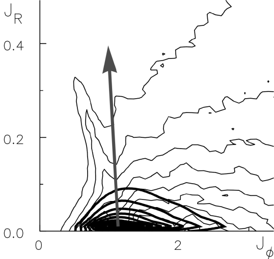
Figure 6.— Map of the norm of the total flux summed over the three resonances (ILR, CR, OLR) (bold lines). The contours are spaced linearly between 95% and 5% of the function maximum. The gray vector gives the direction of the vector flux associated to the norm maximum (arbitrary length). The background contours correspond to the diffused distribution from S12 (thin lines), which exhibits a narrow ridge of diffusion.

4.2. Reproducing the S12 simulation

In this section we examine the extent to which our analytic results can explain the simulations of tapered Mestel discs described by S12. We do not expect perfect agreement between our results and the numerical experiments because we have employed several approximations. In particular we have assumed that the driving fluctuations are white noise that has an amplitude squared that is proportional to the disc’s surface density. We have assumed, moreover, that these fluctuations drive tightly-wound waves. S12 restricted disturbing forces to $m_{\phi}=2$, so we impose this same restriction on ${\bf m}$.

The dark contours in Fig. 6 show the magnitude of the diffusive flux that is generated by the two Lindblad resonances and corotation when one adopts the same numerical pre-factors as S12. The gray arrow shows the direction of the diffusive flux at the location of the peak flux; the direction is similar at neighbouring points. The thin contours in Fig. 6 show the value of the distribution function in S12 after diffusion has taken place. Originally the DF peaked along the $J_{\phi}$ axis at $J_{\phi}\simeq 1$, becoming small to the left of that point on account of the inner taper. Above the location of the peak DF, there is a prominent horn of enhanced stellar density that extends roughly in the direction of the diffusive flux. Thus our analytic results are in good qualitative agreement with the numerical experiments of S12.

In Fig. 6 waves at ILR drive diffusion parallel to vectors that are inclined by $153^{\circ}$ to the $J_{\phi}$ axis, whereas the net flux makes an angle of $111^{\circ}$ with the axis. That these angles are similar attests to the dominant role of waves that have ILR near where the DF peaks. This dominance arises because $\partial f_{0}/\partial J_{r}$ is always negative and in this region $\partial f_{0}/\partial J_{\phi}>0$, so $|{\bf m}\cdot{\partial f_{0}/\partial{\bf J}}|$ is larger for the waves at ILR, which have $m_{r}=-1$, than for the waves at OLR, while $\widetilde{c}_{\bf m}$ is the same for both values of $m_{r}$.

Given that we have assumed that the driving fluctuations are white noise, it is perhaps surprising that the magnitude of the diffusive flux is as sharply peaked in action space as the dark contours in Fig. 6 show it to be. This localisation surely reflects the sharp tapering of the DF at small radii. Just outside this taper the disc becomes significantly self-gravitating and most effective at amplifying the stimulating white noise. The amplified waves tend to have their ILRs further in, where the taper is cutting into the disc.

We have seen that self-gravity amplifies stimuli most strongly at corotation (Fig. 5). In fact, the dominance of corotation increases without limit as $Q$ decreases because the value of $\lambda_{\rm max}$ associated with corotation approaches unity, and the associated amplification diverges, while the value of $\lambda_{\rm max}$ associated with the LRs remains significantly below unity. Fig. 7 illustrates this phenomenon by comparing the velocity of diffusion in action space,

$${\bf v}={{\bf F}\over f},$$ (68)

for two values of $\xi$. For the value $\xi=0.5$ assumed by S12 (left panel) the velocity vectors are significantly non-zero only within the narrow strip at $J_{\phi}\sim 1$ associated with the ILR and point up and to the left. For $\xi=0.73$ the velocity is also quite large at $J_{\phi}>2$ near the $J_{\phi}$ axis and is there directed up and to the right.

Figure 7.— Velocity ${\bf v}\equiv{\bf F}/f$ of the probability density in the $(J_{\phi},J_{r})$ plane for two values of the active fraction of the disc mass: $\xi=0.5$ (left) and $\xi=0.73$ (right). The flux vectors ${\bf F}$ are obtained by summing over all three resonances (ILR, CR, OLR). As $\xi$ increases the CR becomes more important and the main growth in ${\bf v}$ occurs at $J_{\phi}\simeq 2$.

5. Conclusions

In a star cluster or a galaxy stars move on orbits in the system’s mean gravitational field, but the orbit each star is on evolves slowly in response to fluctuations in the mean field (Weinberg, 2001a). In a hot stellar system such as a star cluster, the dominant fluctuations are pure shot noise arising from the finite number of stars in the system. In a disc galaxy the situation is much more complex and interesting because the system’s response is more frequency-sensitive, and as Toomre’s $Q\to 1$ stimuli are strongly amplified and distorted by the coherent responses they induce in the disc.

The orbit-averaged Fokker-Planck equation, which describes the evolution of the distribution function as stars diffuse through action space, provides the mathematical device of choice to compute the long-term evolution of a stellar system. The equation is readily solved once the diffusion tensor has been computed.

We have laid out the general formalism for computing the diffusion tensor in the presence of significant coherent response to stimuli, and have implemented this formalism in the case of a razor-thin, cool disc. By introducing a set of basis functions for the disc’s potential that comprise sets of localised, tightly wound spirals, we have derived equation (52), which reduces computation of the diffusion tensor to execution of a one-dimensional integral over the auto-correlation function of the stimulating noise.

We used this equation to compute the diffusion tensor for a Mestel disc that has been trimmed at both large and small radii by tapers and is exposed to shot noise. We find that diffusive flux shows quite sharp peaks in action space. When Toomre’s parameter $Q$ is significantly bigger than unity, the diffusive flux is quite localised near the inner taper, and is primarily driven by waves that have their inner Lindblad resonances there. This result is interesting in relation to the N-body simulations of S12 because in these simulations, orbital diffusion led to the formation of a horn of enhanced density in phase space that lies close to the region in which our analytic work predicts that the diffusive flux peaks. Moreover, the direction along the horn is similar to the predicted direction of the diffusive flux. Thus it appears that our analytic work recovers quite well the main feature of the simulations.

As $Q$ approaches unity, the corotation resonances of waves become more important because self-gravity amplifies perturbations at corotation very strongly. Waves that are in corotation at some point in action space drive diffusion parallel to the angular-momentum axis of action space, i.e. they drive radial migration. By contrast, waves that are at a Lindblad resonance heat the disc by driving stars to higher eccentricity, while either decreasing (at ILR) or increasing (at OLR) angular momentum. Consequently, our calculations predict that the amount of radial migration for a given level of heating increases as $Q$ decreases towards unity.

In our application of action-space diffusion to cool discs, the disc’s response to stimuli has been restricted to tightly-wound spirals. This restriction unfortunately excludes from consideration the key physics of “swing amplification” at corotation (Toomre, 1981). As Goldreich & Lynden-Bell (1965) originally showed in the context of a gas disc, leading waves are amplified at corotation as they morph into trailing waves. These waves will then propagate to the Lindblad resonances and there heat the disc (Toomre, 1981). Shot noise will stimulate leading waves in the same amount as trailing waves, and the leading waves will move to corotation rather than to the Lindblad resonances, and there morph into trailing waves of larger amplitude. Our computation has not included the effect of swing-amplification at corotation, and will consequently under-estimate the extent of heating. The under-estimation will be largest for small values of $Q$, because swing amplification diverges as $Q\to 1$.

Another shortcoming of the present analysis is the crude noise model which has ad-hoc dependence on the temporal frequency $\nu$ and the radial wavenumber $k_{r}$, and is only a function of the position in the disc through $J_{\phi}$. The model aims to reproduce the Poisson shot noise caused by the finite number of particles in the disc. In a companion paper, we will investigate the WKB limit of the Balescu-Lenard equation. This approach will allow us to avoid such approximation since it naturally captures the intrinsic noise, due to finite$-N$ effects, and its impact on the quasi-stationnary distribution function, as long as the evolution of the system is made through transient tightly wound spirals.

In a forthcoming paper we will use the present formalism of forced diffusion to study the evolution of a stellar disc as a result of cosmic noise: the noise generated by satellites that orbit in a disc’s host dark halo.

Another possible application of the formalism developed here is to study the secular evolution of dark-matter cusps at the centres of galaxies in response to stochastic excitation by the inner baryonic disc and bulge. (Fouvry et al., 2014b).

This paper is dedicated to the memory of Jean Heyvaerts who was its inspiration.

Acknowledgements

JBF thanks the GREAT program for travel funding. CP thanks the Institute of Astronomy, Cambridge, for hospitality while this investigation was initiated. We thank S. Colombi, S. Prunet and P. H. Chavanis for comments. This work is partially supported by the Spin(e) grants ANR-13-BS05-0005 of the French Agence Nationale de la Recherche and by the ILP LABEX (under reference ANR-10-LABX-63) which is funded by ANR-11-IDEX-0004-02. The research leading to these results has received funding from the European Research Council under the European Union’s Seventh Framework Programme (FP7/2007-2013) / ERC grant agreement no. 321067.

References

- Aubert & Pichon (2007) Aubert, D., & Pichon, C. 2007, MNRAS, 374, 877
- Aumer & Binney (2009) Aumer, M., & Binney, J. J. 2009, MNRAS, 397, 1286
- Binney (2010) Binney, J. 2010, MNRAS, 401, 2318
- Binney (2013) —. 2013, Dynamics of secular evolution, ed. J. Falcón-Barroso & J. H. Knapen (Cambridge University Press), 259
- Binney (2014) —. 2014, MNRAS, 440, 787
- Binney & Lacey (1988) Binney, J., & Lacey, C. 1988, MNRAS, 230, 597
- Binney & Tremaine (2008) Binney, J., & Tremaine, S. 2008, Galactic Dynamics: (Second Edition), Princeton Series in Astrophysics (Princeton University Press)
- Born (1960) Born, M. 1960, The Mechanics of the Atom (F. Ungar Pub. Co.)
- Chavanis (2012) Chavanis, P. H. 2012, European Physical Journal Plus, 127, 19
- Daubechies (1990) Daubechies, I. 1990, Information Theory, IEEE Transactions on, 36, 961
- Dehnen (1998) Dehnen, W. 1998, AJ, 115, 2384
- Eyre & Binney (2011) Eyre, A., & Binney, J. 2011, MNRAS, 413, 1852
- Famaey et al. (2005) Famaey, B., Jorissen, A., Luri, X., et al. 2005, A&A, 430, 165
- Fouvry et al. (2014a) Fouvry, J. B., Pichon, C., & Prunet, S. 2014a, in press
- Fouvry et al. (2014b) Fouvry, J. B., et al. 2014b, in prep
- Gabor (1946) Gabor, D. 1946, Electrical Engineers - Part III: Radio and Communication Engineering, Journal of the Institution of, 93, 429
- Goldreich & Lynden-Bell (1965) Goldreich, P., & Lynden-Bell, D. 1965, MNRAS, 130, 125
- Helmi & White (1999) Helmi, A., & White, S. D. M. 1999, MNRAS, 307, 495
- Kalnajs (1965) Kalnajs, A. J. 1965, Ph.D. thesis (Harvard University)
- Kalnajs (1971) —. 1971, ApJ, 166, 275
- Lin & Shu (1966) Lin, C. C., & Shu, F. H. 1966, Proceedings of the National Academy of Science, 55, 229
- McMillan (2013) McMillan, P. J. 2013, MNRAS, 430, 3276
- Mestel (1963) Mestel, L. 1963, MNRAS, 126, 553
- Pichon & Aubert (2006) Pichon, C., & Aubert, D. 2006, MNRAS, 368, 1657
- Piffl et al. (2014) Piffl, T., Binney, J., McMillan, P. J., et al. 2014, ArXiv e-prints, arXiv:1406.4130
- Sanders & Binney (2013) Sanders, J. L., & Binney, J. 2013, MNRAS, 433, 1826
- Schönrich & Binney (2009) Schönrich, R., & Binney, J. 2009, MNRAS, 396, 203
- Sellwood (2010) Sellwood, J. A. 2010, MNRAS, 409, 145
- Sellwood (2012) —. 2012, ApJ, 751, 44
- Sellwood & Binney (2002) Sellwood, J. A., & Binney, J. J. 2002, MNRAS, 336, 785
- Sellwood & Carlberg (2014) Sellwood, J. A., & Carlberg, R. G. 2014, ApJ, 785, 137
- Toomre (1964) Toomre, A. 1964, ApJ, 139, 1217
- Toomre (1977) —. 1977, ARA&A, 15, 437
- Toomre (1981) Toomre, A. 1981, in Structure and Evolution of Normal Galaxies, ed. S. M. Fall & D. Lynden-Bell, 111–136
- Weinberg (2001a) Weinberg, M. D. 2001a, MNRAS, 328, 311
- Weinberg (2001b) —. 2001b, MNRAS, 328, 321
- Wielen (1977) Wielen, R. 1977, A&A, 60, 263