Gas flow in barred potentials II. Bar Driven Spiral Arms.

Abstract

Spiral arms that emerge from the ends of a galactic bar are important in interpreting observations of our and external galaxies. It is therefore important to understand the physical mechanism that causes them. We find that these spiral arms can be understood as kinematic density waves generated by librations around underlying ballistic closed orbits. This is even true in the case of a strong bar, provided the librations are around the appropriate closed orbits and not around the circular orbits that form the basis of the epicycle approximation. An important consequence is that it is a potential’s orbital structure that determines whether a bar should be classified as weak or strong, and not crude estimates of the potential’s deviation from axisymmetry.

1 Introduction

Many grand design barred spirals exhibit spiral arms starting at and extending out from the end of the bar. How are these spiral arms generated? The natural interpretation is that they are driven by the bar. The spiral arms and the bar must also be rotating at the same pattern speed if the starting points of the arms always coincide with the bar’s ends. Such spiral arms are relevant for the interpretation of observations of both our Galaxy and external galaxies. For example, it is likely that some features present in spectral-line emission of atomic and molecular gas in the inner Galaxy, for instance the “3kpc arm”, are produced by such arms (Dame & Thaddeus, 2008, e.g.). It is therefore important to have a physical understanding of why such spiral arms arise.

On the theoretical side, the possibility of bar-driven spiral arms is now well established. The first investigations used analytical methods and were carried out by Feldman & Lin (1973) and Lin & Lau (1975). Then, in the following years, Sanders & Huntley (1976); Sanders (1977) and Huntley et al. (1978) performed pioneering numerical experiments and discussed the physical mechanism responsible for the generation of the spiral arms in terms of closed orbits. Their work was later extended independently by Wada (1994) and Lindblad & Lindblad (1994), and more recently by Piñol-Ferrer et al. (2012). These authors constructed phenomenological analytical models under the epicyclic approximation with the purpose of understanding the spiral arms. In their models gas parcels follow weakly oval orbits, whose major axes orientation changes with radius giving rise to kinematic density waves a-la Lindblad, and hence to spiral arms.

An alternative viewpoint which does not consider the spiral arms as density waves has also been discussed in a series of papers by Romero-Gómez et al. (2006, 2007); Athanassoula et al. (2009a, b, 2010). Their theory, which is more directly applicable to stars than to gas, is based on the observation that orbits in the vicinity of unstable Lagrangian points can be trapped into invariant manifolds whose morphology can reproduce the spiral arms.

Many authors have noted the presence of bar-driven spiral arms in simulations, and discussed them in a more or less descriptive way (see for example Athanassoula, 1992; Englmaier & Gerhard, 1999; Bissantz et al., 2003; Rodriguez-Fernandez & Combes, 2008). For a recent review see also Section 2.3 of Dobbs & Baba (2014). Note that in all works cited above the gas is driven by an external potential generated by the bar and is not self-gravitating, and therefore the spiral arms are not spiral density waves in the sense of Lin & Shu (1964). We do not discuss self-gravity in this work.

The viewpoint that spiral arms can be understood as density waves is nowadays often assumed, but has never been tested with sufficient detail. On modern computers, it is very cheap to run simulations able to test the predictions and the limits of the phenomenological models cited above. Moreover, the literature only addresses the weak bar regime under the epicyclic approximation, and does not discuss how the picture should be extended to the strong bar case.

In this paper we investigate the physical mechanism responsible for the generation of the spiral arms and in particular we resume the discussion of how they can be understood as kinematic density waves. The structure is as follows. In Sec. 2 we briefly review previous work aimed at understanding in a phenomenological fashion the spiral arms in the epicyclic approximation. Then we run grid based, isothermal, non-self gravitating 2D hydrodynamic simulations in an externally imposed rigidly rotating barred potential, addressing both the weak and the strong bar case. The numerical methods employed are explained in Section 3. In Sec. 4 we compare the results of the simulations with the phenomenological models available in the literature. In Sec. 5 we discuss in more detail the weak bar case, and in Sec. 6 how the results for the weak bar case should be extended to the strong bar case. Finally, we summarise our findings in Sect. 7.

2 Review of previous work

In this section we briefly review previous work aimed at understanding the bar driven spiral arms in the epicycle approximation. In Sec. 2.1 we discuss the equations describing ballistic closed orbits in the epicycle approximation (see for example Sect. 3.3.3 in Binney & Tremaine, 2008). In Sec. 2.2 we discuss how various authors have modified the ballistic equations in order to describe gaseous parcels, and the phenomenological models based on these equations. These phenomenological models will be in later sections compared with the results of hydro simulations.

2.1 Ballistic closed orbits in the epicycle approximation

Consider a rigidly rotating external potential of the form

$$\Phi(R,\theta)=\Phi_{0}(R)+\Phi_{1}(R,\theta)\;,$$ (1)

where $\Phi_{0}$ is an axisymmetric potential and $\Phi_{1}$ is a small but otherwise arbitrary perturbation. The potential is assumed to be rigidly rotating at pattern speed $\Omega_{\rm p}$. $R,\theta$ are polar coordinates in the rotating frame, with $\theta=0$ corresponding to the positive horizontal axis, and $\theta$ increasing clockwise. The equation of motion for a ballistic particle in this potential is

$$\ddot{\mathbf{x}}=-\nabla\Phi+\Omega_{\rm p}^{2}\mathbf{x}-2\Omega_{\rm p}\left(\hat{\mathbf{e}}_{z}\times\dot{\mathbf{x}}\right)\;,$$ (2)

where $\hat{\mathbf{e}}_{z}$ is the unit vector perpendicular to the plane. The first term on the RHS represents gravitational forces, the second term is the centrifugal force and the third is the Coriolis force.

We want to find closed orbits in the above potential under the epicycle approximation. In the absence of the perturbation $\Phi_{1}$ the potential is axisymmetric and the only stable closed orbits are circular orbits. These circular orbits will be described in polar form as

$$R(t) =R_{0}\;,$$ (3)

$$\theta(t) =\theta_{0}(t)=\Omega_{\rm f}t\;,\qquad$$ (4)

where

$$\Omega_{\rm f}=\Omega-\Omega_{\rm p}\;,$$ (5)

and $\Omega=\Omega(R_{0})$ is the angular velocity for circular motion at radius $R_{0}$ in the potential $\Phi_{0}$. Now consider the situation in the presence of the small perturbation $\Phi_{1}$. We want orbits that are closed in the rotating frame. We expect that far from resonances closed orbits will be weak oval deformations of the circular orbits found in $\Phi_{0}$. We look for closed orbits of the form

$$R(t) =R_{0}+R_{1}(t)\;,$$ (6)

$$\theta(t) =\theta_{0}(t)+\theta_{1}(t)\;,$$ (7)

where all quantities with subscript $1$ are to be considered small. By expressing Eq. (2) in polar components, then substituting Eqs. (6), (7) and (1) into it and approximating to first order in quantities with subscript $1$, the equations of motion take the following form:

$$\ddot{R}_{1}+\left(\frac{\mathrm{d}^{2}\Phi_{0}}{\mathrm{d}R^{2}}-\Omega^{2}\right)_{R_{0}}R_{1}-2R_{0}\Omega\dot{\theta}_{1}=-\left(\frac{\partial\Phi_{1}}{\partial R}\right)_{R_{0},\theta_{0}(t)}\;,$$ (8)

$$\ddot{\theta}_{1}+2\Omega\frac{\dot{R}_{1}}{R_{0}}=-\frac{1}{R_{0}^{2}}\left(\frac{\partial\Phi_{1}}{\partial\theta}\right)_{R_{0},\theta_{0}(t)}\;,$$ (9)

where the derivatives of $\Phi_{1}$ are evaluated along the unperturbed trajectory $[R_{0},\theta_{0}(t)]$ and are therefore to be considered given functions of time. Exploiting the fact that $\theta_{0}(t)$ is a linear function of time, Eq. (9) can be integrated immediately to obtain $\dot{\theta}_{1}$, which can then substituted into Eq. (8). This gives

$$\boxed{\ddot{R}_{1}+\kappa_{0}^{2}R_{1}=f_{1}(t)},$$ (10)

where

$$\kappa_{0}^{2} =\left(R\frac{\mathrm{d}\Omega^{2}}{\mathrm{d}R\,\,}+4\Omega^{2}\right)_{R_{0}}\;,$$ (11)

$$f_{1}(t) =-\left[\left(\frac{\partial\Phi_{1}}{\partial R}\right)+\frac{2\Omega}{\Omega_{\rm f}R_{0}}\Phi_{1}\right]_{R_{0},\theta_{0}(t)}\;.$$ (12)

Eq. 10 is the equation of a forced harmonic oscillator. The natural frequency of this oscillator is $\kappa_{0}$, the usual epicycle frequency that can be calculated from $\Phi_{0}$. The driving force is $f_{1}(t)$, and as one would expect it is due to the perturbing potential $\Phi_{1}$ and reduces to zero when this is turned off. $f_{1}(t)$ is a periodic function of time. If we expand it in its Fourier components with respect to time, we will find the same components contained in the Fourier expansion of $\Phi_{1}$ with respect to $\theta$. This is not surprising, as the perturbed potential encountered by the guiding centre of the ballistic particle is given by $\Phi_{1}(R_{0},\theta_{0}(t))$ where $\theta_{0}(t)$ increases linearly with time.

The general solution of Eq. (10) could in principle be easily written down. For each solution, we could eliminate $t$ from Eqs. (6), (7) to find the orbit in the form $R=R(\theta)$. Not all solutions of Eq. (10) correspond in general to closed orbits in the rotating frame. Some particular solutions describe closed orbits, while the others in general describe non closed loop orbits. The first type of solution are the ballistic closed orbits in the epicycle approximation.

For concreteness, let us now consider the particular form of the potential used by Sanders (1977) and Wada (1994):

$$\Phi_{0}(R)=-\frac{av_{0}^{2}}{\sqrt{R^{2}+a^{2}}}\;,$$ (13)

$$\Phi_{1}(R,\theta)=\Phi_{\rm b}(R)\cos(2\theta)\;,\qquad\Phi_{\rm b}(R)=-\epsilon\frac{(av_{0}R)^{2}}{(R^{2}+a^{2})^{2}}\;,$$ (14)

where $a$, $v_{0}$, $\epsilon$ are constant parameters. The axisymmetric part $\Phi_{0}$ is a Kuzmin-Toomre potential, and the perturbation $\Phi_{1}$ was introduced by Sanders (1977). Following Wada (1994), we choose $a=1\,{\rm kpc}$ and $v_{0}=100\,{\rm km\,s^{-1}}$ and a pattern speed of $\Omega_{\rm p}=10\,{\rm km\,s^{-1}}\,{\rm kpc}^{-1}$. Different values of $\epsilon$ will be considered in the following. Fig. 1 shows the circular speed curve and the behaviour of $\Omega-n\kappa_{0}/2$, from which we can determine the location of the resonances, for this choice of values of the parameters. For this potential, Eq. (10) becomes

$$\boxed{\ddot{R}_{1}+\kappa_{0}^{2}R_{1}=f_{\rm w}\cos(2\Omega_{\rm f}t)}\;,$$ (15)

where

$$f_{\rm w}(R_{0})=-\left[\left(\frac{\mathrm{d}\Phi_{\rm b}}{\mathrm{d}R}\right)+\frac{2\Omega}{\Omega_{\rm f}R_{0}}\Phi_{\rm b}\right]_{R_{0}}.$$ (16)

The forcing is now a periodic function of time with frequency $2\Omega_{\rm f}$. By solving (15), it is found that ballistic closed orbits have the major axis always either perpendicular or parallel to the major axis of the bar. The orientation changes abruptly at each ILR, at CR, and at OLR. Note however that the above analysis is not valid in the vicinity of these points: at all Lindblad resonances the natural frequency of the oscillator $2\Omega_{\rm f}$ tends to the forcing frequency $\kappa_{0}$, while at CR the forcing $f_{\rm w}$ becomes infinite. The orientation of the ballistic closed orbits will be important in the next subsection.

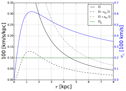
Figure 1: Blue curve: circular speed curve for the potential in Eq. (13) with values of parameters indicated in the text. Black curves: behaviour of $\Omega-n\kappa_{0}/2$ for the same potential. The horizontal green line indicates the assumed value of the pattern speed.

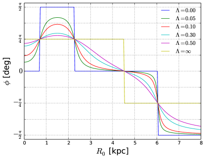
Figure 2: Predictions of Wada’s model for the phase $\phi$ as function of guiding-centre radius $R_{0}$ for the potential in Eq. (13). $\phi$ represents the orientation of the major axis of a closed orbit. Curves corresponding to different values of the damping parameter $\Lambda$ are shown. The possible values allowed by the phenomenological model are enclosed between the blue and yellow lines.

2.2 Gaseous closed orbits in the epicycle approximation: phenomenological models

In the previous section we have seen that for the particular potential given by Eqs. (13) and (14) the significant ballistic closed orbits are always oriented either perpendicularly or parallel to the major axis of the bar, with abrupt changes of orientation at each resonance. However, the discussion was only valid for ballistic particles. How should we modify it to describe the motion of a gaseous parcel which is part of a continuous fluid? Sanders & Huntley (1976) suggested that in the gaseous case the orientation shift between horizontally and vertically aligned orbits happens gradually, and that this gives rise to kinematic spiral arms a-la Lindblad. Moreover, they noted that the addition of a dissipation term to Eq. (15),

$$\boxed{\ddot{R}_{1}+2\lambda\dot{R}_{1}+\kappa_{0}^{2}R_{1}=f_{\rm w}\cos\left(2\Omega_{\rm f}t\right)}\;,$$ (17)

can remove the divergence of the radial oscillation amplitude at the Lindblad resonaces, and that the solution of Eq. (17) where transients are neglected always describes a closed orbit. They also noted that at each ILR, the closed orbit solution so obtained has a major axis inclined at $\pi/4$ independently of the value of $\lambda$. Since $\pi/4$ is halfway between horizontally and vertical elongated orbits, this corroborated the conjecture that in the gaseous case we expect a gradual shift from vertically elongated to horizontally elongated when we cross a Lindblad resonance, which is the key to the generation of spiral arms in their model.

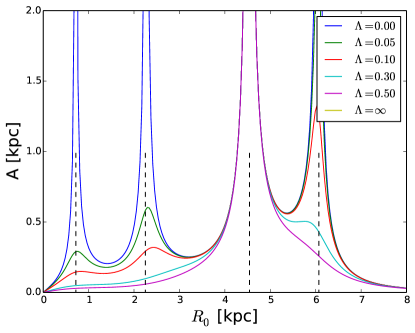
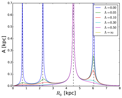
Figure 3: Amplitude of the radial oscillations predicted by Wada’s model for two different values of the bar strength $\epsilon$. The top panel is for $\epsilon=0.05$, and the bottom panel is for $\epsilon=0.005$. In each panel, curves corresponding to different values of the damping parameter $\Lambda$ are shown. In absence of a damping term, $\Lambda=0$, the amplitude diverges at all Lindblad resonances and at corotation. The presence of a damping term makes the amplitude finite at the Lindlblad resonances, but not at corotation.

Wada (1994) and Lindblad & Lindblad (1994); Piñol-Ferrer et al. (2012) independently developed further this idea by taking more seriously the dissipation term, considering it as a phenomenological model that describes the trajectory of gaseous particles over extended regions. The approaches of Wada (1994) and Lindblad & Lindblad (1994) differ slightly in the way they implement the dissipation term. The phenomenological model of Wada (1994) is based exactly on Eq. (17). This amounts to add a dissipation term for the motion of the particle in the radial direction only. Lindblad & Lindblad (1994) added a dissipation term that is proportional to the difference between the velocity of the particle and the local circular speed in the underlying axisymmetric potential. Here, we consider in more detail the variant of Wada (1994), but the results of the Lindblad & Lindblad (1994) variant are qualitatively similar, and a more detailed account of the results using this variant can be found in Piñol-Ferrer et al. (2012).

Let us now briefly review Wada’s model. The solution of Eq. (17) that excludes transient terms yields closed orbits of the following form:

$$R(\theta)=R_{0}+A\cos 2\left(\theta-\phi\right)\;,$$ (18)

where the amplitude is

$$A=\frac{|f_{\rm w}|}{F}\;,$$ (19)

with

$$F=\sqrt{\left[\kappa_{0}^{2}-\left(2\Omega_{\rm f}\right)^{2}\right]^{2}+\left(4\lambda\Omega_{\rm f}\right)^{2}}\;.$$ (20)

The phase $\phi$ in (18) is given by the solution of

$$\begin{split}\sin 2\phi&=\frac{4\lambda|\Omega_{\rm f}|}{F}\text{sign}(f_{\rm w})\;,\\ \ \cos 2\phi&=\frac{\kappa_{0}^{2}-\left(2\Omega_{\rm f}\right)^{2}}{F}\;,\ \end{split}$$ (21)

that lies in the range $-\pi\leq 2\phi\leq\pi$. It encodes the information about the orientation of the major axis of the closed orbit, and is the inclination of the major axis of the orbit with respect to the horizontal axis. From Eq. (21) we see that the quadrant $2\phi$ belongs to is determined by the sign of $f_{\rm w}$, which flips at CR, and by the sign of $\kappa_{0}^{2}-2\Omega_{\rm f}^{2}$, which flips at each Lindblad resonance. The phase $\phi$ in Eq. (18) is determined for all orbits once $\lambda=\lambda(R_{0})$ is given at each radius. Since $\lambda$ has the dimension of a frequency, it is convenient to express it as a multiple of a characteristic frequency at that radius. Following Wada (1994), we express $\lambda$ as a multiple of the epicycle frequency at that radius, namely

$$\lambda=\Lambda\kappa_{0}\;.$$ (22)

Fig. 2 reproduces Fig. 2 of Wada (1994) and shows his model predictions for the phase $\phi$ for different constant values of $\Lambda$. In the limit $\Lambda\to 0$ we recover the ballistic case, while in the limit $\Lambda\to\infty$ all orbits are circular. The curves $\Lambda=0$ and $\Lambda=\infty$ bound the possible values that the $\phi$ can assume in its model. Note that this plot does not depend on the strength of the bar potential $\epsilon$, because the phase $\phi$ does not depend on the magnitude of $f_{\rm w}$ but only on its sign.

$A$ is the amplitude of radial oscillations. Fig. 3 shows the amplitude $A$ of the radial oscillations predicted by the model for various values of $\Lambda$ and two different values of $\epsilon$. As can be seen from this figure, $A$ always diverges at CR, regardless of the value of $\Lambda$, but diverges at the Lindblad resonances only in the absence of the damping term. Note also that, for given $\epsilon$, away from resonances the value of $A$ is limited from above: the maximum value that $A$ can reach at given $R_{0}$ is limited by its value for $\Lambda=0$. Finally, note that for a given potential, this theory has only one adjustable parameter at each radius, the damping $\lambda$. Both $\phi$ and $A$ at each radius depend on a single phenomenological parameter in this theory.

Using the theory outlined above, it is possible to construct explicit models of the spiral arms. Fig. 4, top panels, reproduces the model shown in Fig. 4 of Wada (1994). It shows a nested sequence of closed orbits for values of the parameters $\epsilon=0.05$ and $\Lambda=0.05$. The bottom panels show another model, for a weaker bar $\epsilon=0.005$ and $\Lambda=0.02$.

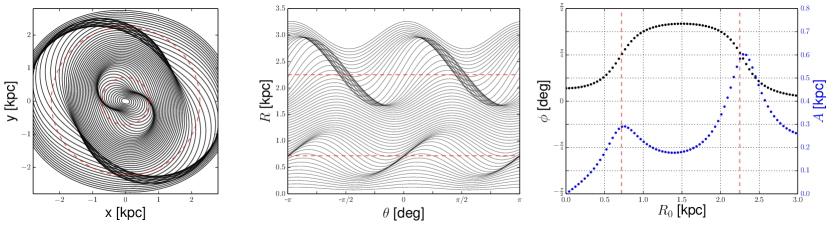
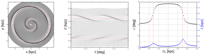
Figure 4: Top: reproduction of Wada (1994) predictions for a bar strength of $\epsilon=0.05$. The damping parameter is $\Lambda=0.05$. Bottom: another model produced using Wada (1994) theory, for $\epsilon=0.005$ and $\Lambda=0.02$.

3 Numerical methods

In our simulations, we assume that the gas is a fluid governed by the Euler equations complemented by the equation of state of an isothermal ideal gas. Then we run two-dimensional hydrodynamical simulations in an externally imposed, rigidly rotating barred potential. The output of each simulation consists in snapshots of the velocity and surface density distributions $\rho(\mathbf{x})$ and $\mathbf{v}(\mathbf{x})$ at chosen times.

We use a grid-based, Eulerian code based on the second-order flux-splitting scheme developed by van Albada et al. (1982) and later used by Athanassoula (1992), Weiner & Sellwood (1999) and others to study gas dynamics in bar potentials. We used the same implementation of the code as was used by Sormani et al. (2015), which also implements the recycling law of Athanassoula (1992).

We used a grid $N\times N$ to simulate a square $8\,\,{\rm kpc}$ on a side. $N$ depends on the resolution of the simulation. The initial conditions of the runs are as follows. We start with gas in equilibrium on circular orbits in an axisymmetrized potential and, to avoid transients, turn on the non-axisymmetric part of the potential gradually. We use outflow boundary conditions: gas can freely escape the simulated region, after which it is lost forever. The potential well is sufficiently deep, however, to prevent excessive quantities of material to escape.

The recycling law introduces a term in the continuity equation that was originally meant to take into account in a simple way the effects of star formation and stellar mass loss. The equation governing this process is

$$\frac{\partial\rho}{\partial t}=\alpha(\rho_{0}^{2}-\rho^{2})\;,$$ (23)

where $\alpha=0.3\,M_{\odot}\,{\rm pc}^{-2}\,{\rm Gyr}^{-1}$ is a constant and $\rho_{0}$ is the initial surface density, which is taken to be $\rho_{0}=1\,M_{\odot}\,{\rm pc}^{-2}$. In practice, the only effect of the recycling law is to prevent too much gas accumulating in the very centre and to replace gas lost at the boundary due to the outflow boundary conditions. It does not affect the morphology of the results, so our results do not change if we disable the recycling law.

4 Phenomenological Models vs Hydro simulations

What happens if we run a simulations in the potential of Eqs. (13) and (14)? Do the results of a hydro simulation resemble the predictions of the phenomenological models? Fig. 5 answers this question. It shows the results of a simulation in which $\epsilon(t)$ is a slowly changing function of time. At $t=0$ we have $\epsilon=0$, then $\epsilon$ increases linearly with time until it reaches Wada’s value of $\epsilon=0.05$ at $t=12.3\rm Gyr$, and for later times it is kept constant at this value. The potential evolves so slowly that the gas flow configuration evolves almost adiabatically, adjusted to the instantaneous underlying potential. In other words, at each time $t$ the gas configuration is almost the same as the steady state configuration that would be obtained by freezing the potential and then waiting for the gas to settle down into a steady state.

At early times, when $\epsilon$ is very small, the results of the hydro simulation do qualitatively resemble the predictions of the phenomenological models, as can be seen by comparing the top row in Fig. 5 with Fig. 4. At later times, when $\epsilon$ is greater, this is not true: for example panels in the bottom row do not look like Wada (1994) predictions. Inspection of streamlines shows that for very small values of $\epsilon$ the gas is flowing on almost circular orbits, as the epicycle approximation requires, but when $\epsilon$ becomes larger the gas flows instead on very horizontally elongated orbits, and the epicycle approximation is not valid anymore. How can we explain this behaviour? Why does the gas flow on very elongated orbits despite the fact that the perturbation is apparently very small? As we shall now see, the key to answer these questions lies in the orbital structure of the underlying potential.

Fig. 6 shows how the orbital structure of the underlying potential changes as $\epsilon$ is varied. Each row refers to a particular value of $\epsilon$. Let us first consider the top row, which shows the case $\epsilon=0$, when the bar perturbation is turned off and the potential is exactly axisymmetric. Consequently, orbits that close in our rotating frame are either circular or they are orbits for which the precession frequency happens to coincide with our chosen “pattern speed”, which is actually of no physical significance when $\epsilon=0$. The top left panel of Fig. 6 shows several families of closed orbits: each dot represents a closed orbit in terms of its value of the Jacobi constant $E_{j}$ and the coordinate at which the orbit cuts the vertical axis. All the orbits shown in this diagram (known as characteristic diagram, see Contopoulos & Grosbol, 1989) have the property of cutting the vertical axis at right angles. The line of dark dots shows the circular orbits. Since for $\epsilon=0$ the potential is axisymmetric, these are the only stable closed orbits.

The red crosses in the top left panel of Fig. 6 show eccentric orbits that close in the rotating frame. Such orbits exist only between the two ILRs. They spring out from the sequence of nearly circular orbits at a radius of the innermost inner Lindblad resonance ILR1, and then merge into it again at a bigger radius corresponding to the other inner Lindblad resonance, ILR2. The red crosses that are above the dark line are elongated perpendicularly to the bar, while those below it are elongated along the bar. In fact, since the potential is axisymmetric, the red cross above the dark line and that vertically below it represent orbits that differ only in a $90^{\circ}$ rotation of the major axis. Since the potential is axisymmetric, it is actually possible to find equivalent orbits for any orientation, but these are not shown in the diagram as they do not cut the vertical axis at right angles. The central panel of Fig. 6 shows how the orbits appear in the $xy$ plane. These orbits are coloured differently according to their value of the Jacobi constant $E_{j}$.

We now consider what happens when a small perturbation is turned on, so the potential is no longer exactly axisymmetric. The left panel of the second row of Fig. 6 shows that for $\epsilon=0.005$, a bifurcation is present approximately at the location of ILR1. The line of dark points that marks the circular orbits in the axisymmetric case is now split. The part inside ILR1 merged with what used to be the orbits elongated along the bar in the axisymmetric case (which have become stable) to form a continuous line. In fact, this continuous line constitutes the $x_{1}$ family in the notation of Contopoulos & Grosbol (1989). The part that used to be circular orbits between the two ILRs now forms a closed loop with the orbits elongated perpendicularly to the bar. In fact, the former circular orbits between the ILRs have become the stable $x_{2}$ family, while the orbits elongated perpendicularly to the bar have become the $x_{3}$ family and have remained unstable, as opposed to the $x_{1}$ orbits that have become stable. Note also that the $x_{3}$ orbits are not the $x_{1}$ orbits rotated as in the axisymmetric case, because the potential is no longer axisymmetric.

When in the bottom two rows of Fig. 6 we further increase $\epsilon$, the $x_{2}$-$x_{3}$ loop shrinks, and has almost disappeared when $\epsilon=0.05$. Note that the shape of the orbits, visible in the central column, does change as we increase $\epsilon$, but not dramatically. What changes significantly is the fraction of the volume of phase space that is occupied by non-closed orbits that librate around $x_{1}$ orbits rather than around $x_{2}$ orbits. The right column of Fig. 6 illustrates this point by showing surfaces of section for a value of Jacobi constant $E_{j}=-0.5$ (for a definition of surfaces of section see for example Chapter 3 in Binney & Tremaine, 2008). When $\epsilon=0$, all non closed orbits are parented by the circular orbit, which corresponds to the centre of the “eye” in the top-right panel. When $\epsilon=0.005$, two eyes are present in the surfaces of section; the centre of the left one corresponds to the $x_{1}$ orbit, the centre of the right one to the $x_{2}$ orbit (which replaces the circular orbit). Some orbits are now parented by the $x_{1}$ orbit, and some others by the $x_{2}$. As we increase $\epsilon$, the $x_{1}$ orbits becomes predominant in the surface of section, and the fraction of orbits parented by it increases until the $x_{2}$ orbit disappears for this energy.

It is now easy to go back to Fig. 5 and interpret the results. When $\epsilon$ is small, the gas is circulating on $x_{2}$ orbits in the outer parts and on weakly elongated $x_{1}$ orbits in the inner part (inside the ILR1). When $\epsilon$ is increased, the volume of phase space occupied by orbits parented by $x_{2}$ orbits is reduced. $x_{2}$ orbits start disappearing at small radii, and as they disappear the gas has no other choice than to settle onto $x_{1}$ orbits. When $\epsilon=0.05$ the $x_{2}$ orbits are gone almost everywhere, and the gas is flowing everywhere on $x_{1}$ orbits, including the region where the $x_{1}$ orbits are highly elongated. In this regime, the epicycle approximation obviously cannot work as the $x_{1}$ orbits are not weakly deformed circular orbits. If we call weak a bar that can be well described under the epicycle approximation, then the $\epsilon=0.05$ case should be classified as a strong bar, despite the fact that the non-axisymmetric part of the potential might naively appear small compared to the axisymmetric part.

We have now two questions.

1. How do the phenomenological theories reviewed above compare with the hydro simulations in the weak bar case, that is, when $\epsilon$ is extremely small and the epicycle approximation is valid?

2. What can we say in the strong bar case, when the gas is flowing on very elongated orbits and the epicycle approximation is not valid?

Sections 5 and 6 investigate these two questions respectively.

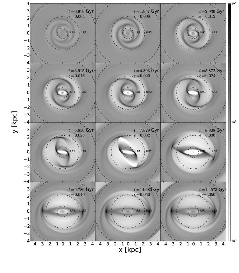
Figure 5: Time sequence for a simulation in the potential defined by Eqs. (13) and (14). Each panel shows the density map at a particular time. The bar strength $\epsilon$ increases slowly and linearly with time until it reaches the value of $\epsilon=0.05$, and is then frozen. The gas adjusts almost adiabatically to the instantaneous underlying potential. The sound speed is $c_{s}=2.5\,{\rm km\,s^{-1}}$ and the spatial resolution is $\mathrm{d}x=20\,{\rm pc}$. The dotted circles indicate the two ILRs and the CR. In each panel, the evolutionary time $t$ and the instantaneous value of $\epsilon$ are shown. The colorbar is in units of $M_{\odot}\,{\rm pc}^{-2}$

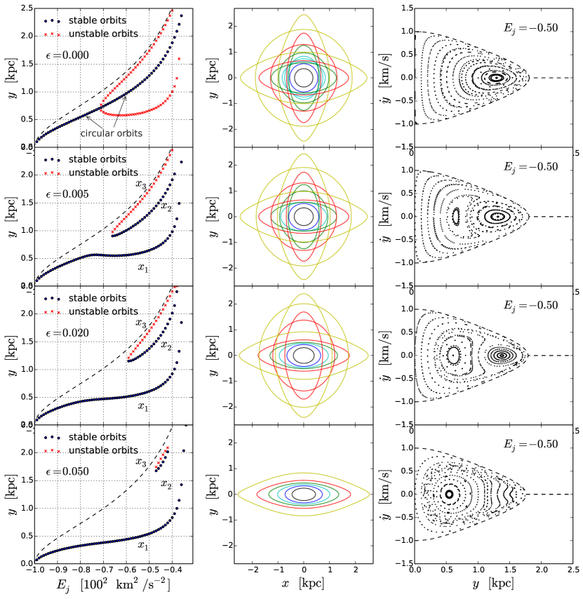
Figure 6: Orbital structure of the potential given by Eq. (13) for different values of $\epsilon$. Rows from top to bottom show the cases $\epsilon=0.0,0.005,0.02,0.05$, respectively. In the left column, the Jacobi constant $E_{j}$ of a closed orbit is plotted against the value at which the orbit cuts the vertical axis in potentials with different values of $\epsilon$. Each dot represents a closed orbit, and all closed orbits cut the vertical axis with purely horizontal velocity. The middle column shows the closed orbits in $xy$ space, with orbits of the same colour having the same energy. The orbits shown are those corresponding to values of $E_{j}$ equal to $\{-0.9,-0.8,-0.7,-0.6,-0.5,-0.4\}$. The vertical slices of the grid in the left panels are drawn at these energies. The correspondence between energy and colours can be identified from the bottom panel in the central column: here greater energy (i.e., less negative) corresponds to bigger orbits, and the same colour coding applies to other panels. The right column shows surfaces of section for $E_{j}=-0.5$.

5 Weak bar Case

In this section we want to investigate how the phenomenological models reviewed above compare in detail with the results of a hydro simulation in the weak bar case, when the epicycle approximation is valid. To do this, we study the case $\epsilon=0.005$. Note that this is a value ten times smaller than the value $\epsilon=0.05$ considered by Wada (1994) and Piñol-Ferrer et al. (2012). As we have seen in the last section, that should actually be considered a strong bar case, because of its orbital structure.

When the sound speed is not too high, the morphology of the density distribution qualitatively resembles the predictions of Wada (1994) shown in Fig. 4. This can be seen from Fig. 7, which shows results of hydro simulations with $\epsilon=0.005$ and different values of the sound speed $c_{s}$. In these simulations the bar strength is frozen after the value $\epsilon=0.005$ is reached, and the snapshots considered are all at $t=2.9\rm Gyr$, long after the bar is fully grown to this value and the gas has long settled down into a steady-state configuration. The left column shows the density distribution. The density distributions for $c_{s}=0.625\,{\rm km\,s^{-1}}$ and $c_{s}=1.25\,{\rm km\,s^{-1}}$ are very similar: it appears as if the gas configuration is tending towards some limiting configuration as $c_{s}\to 0$ at fixed spatial resolution, and that this limiting configuration has much in common with the predictions of the phenomenological models.

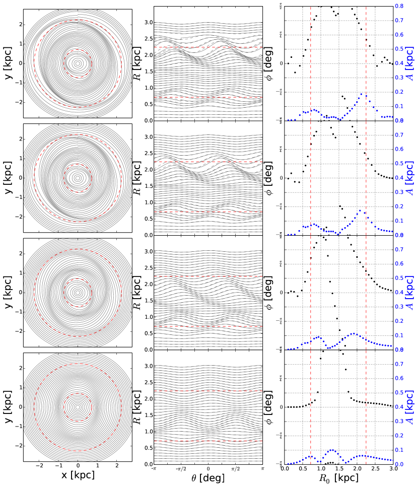
Figure 8: Analysis of the instantaneous streamlines for the snapshots shown in Fig. 7. The left column shows a sequence of nested streamlines in the $xy$ plane. The middle column shows in full lines the same streamlines in the $R\theta$ plane, and in dashed lines the result of a simple fit using Eq. 10, where $A$ and $\phi$ are independent parameters. The right panel shows the best fit values of $A$ and $\phi$ as a function of radius. In each panel the dashed red lines mark the two inner Lindblad resonances.

A second important prediction of the phenomenological model that is confirmed by the hydro simulations is that the spiral arms can be understood as kinematic density waves. Fig. 8 investigates the instantaneous streamlines, that is, the streamlines calculated from a frozen snapshot of the velocity field. Since the gas is in a steady state, these are not much different from the real streamlines followed by gas parcels during the time evolution. We see that in all cases streamlines are almost closed curves, in the sense that in general the mismatch after a single loop is much less than the extent of a radial oscillation during the loop.

Another verified prediction is that streamlines are well described by closed orbits of the form Eq. (18). The middle column in Fig. 8 shows in full lines the same streamlines as the left column in the $R\theta$ plane, and in dashed lines a simple fit to each streamline using Eq. (18) where $A$ and $\phi$ are considered independent free parameters. The streamlines are well fitted by a function of this form, and if we were to reproduce a nested sequence of streamlines as in Fig. 4 using the best fitting values of these two parameters, we would obtain kinematic density waves that reproduce those obtained in the simulation.

However, in the phenomenological models, $A$ and $\phi$ both depend on a single parameter, the dissipation $\lambda$, while in the fitting procedure above $A$ and $\phi$ are treated as independent parameters. Moreover, in the phenomenological models some values of $A$ and $\phi$ are forbidden: $\phi$ must stay within the blue and yellow line in Fig. 2, and the amplitude $A$ away from resonance has an upper bound. Therefore it is not obvious that dissipation parameter $\lambda$ required by the phenomenological model can be tuned for each streamline as to produce the values of $A$ and $\phi$ given by a hydro simulation. In other words, the values obtained from a hydro simulation for $A$ and $\phi$ need not to come from the same value of $\lambda$, or could be outside the regions obtainable for any value of $\lambda$. Indeed, from the right column of Fig. 8 it is clear that in the hydro simulation $A$ and $\phi$ are often outside the regions allowed by the phenomenological models for the same potential. Therefore not all hydro simulations can be reproduced by an appropriate gauging of the dissipation. In fact, we chose to fit using $A$ and $\phi$ as two independent parameters instead of using directly the dissipation $\lambda$ as the only free parameter because $A$ and $\phi$ lie outside the allowed regions too often. However, In the limit of very low sound speed, the results of the hydro simulations for $A$ and $\phi$ are not far from the predictions of the phenomenological model in Fig. 4. The values of $\phi$ in the top two rows of Fig. 8 are more similar than those in other rows to the black dots in the bottom right panel of Fig. 4, and the values of $A$ have also much in common with the blue dots in the same panel, although many are still forbidden because they lie just above the curve $A=0$ in the bottom panel of Fig. 3. Another interesting prediction that is verified in this limit is that the orientation of the major axis of the closed orbits at the two ILRs is $\pi/4$.

Why are the results of the phenomenological models well reproduced in the limit of vanishing sound speed, and less well when the sound speed is higher? To understand this, consider the equations of motion of a gaseous parcel flowing in the hydro simulation. If the fluid were really an ideal isothermal fluid, these would be

$$\frac{D\mathbf{v}}{Dt}=-\nabla\Phi-c_{s}^{2}\frac{\nabla\rho}{\rho}\;,$$ (24)

where $D$ indicates the material derivative, the first term on the right hand side is the gravitational force and the second is the pressure force. However, in a real hydrodynamical simulation at fixed spatial resolution, some unavoidable amount of numerical viscosity, which is not included in Eq. (24), will always be present. This numerical viscosity decreases as we increase the resolution, and tends to zero as the resolution goes to infinity. The equations of motion of a parcel of gas are therefore something like

$$\frac{D\mathbf{v}}{Dt}=-\nabla\Phi-c_{s}^{2}\frac{\nabla\rho}{\rho}-F_{\mathrm{d}x}\;,$$ (25)

where $F_{\mathrm{d}x}$ indicates the force arising from the finite resolution, which we will loosely refer to as the viscous force. Hence, a parcel in a hydro simulation is subject to three different forces: gravitational, pressure and viscosity.

The phenomenological models completely neglect pressure forces. Instead, they only account for the gravitational forces and, phenomenologically, for the viscous forces $F_{\mathrm{d}x}$. Note that the pressure force can be derived from a “pressure potential”

$$\Phi_{P}=c_{s}^{2}\log(\rho/\rho_{0})\;,$$ (26)

where $\rho_{0}$ is an arbitrary number. In a steady-state configuration, the density does not change with time, and the pressure forces can be derived from a static potential. Hence, a gaseous parcel can be considered to move in a potential that is the sum of the gravitational plus the pressure potential. This static pressure potential is not easily derived a priori, and we can only calculate it once we are given the steady-state configuration of the gas after solving the hydrodynamical equations.

The central and right columns in Fig. 7 show the pressure and perturbation potential forces along the horizontal axis. The central column shows forces in the $y$ direction; the gravitational forces in this direction are zero for the chosen form of the perturbation potential. The right column shows forces in the horizontal direction. We see that at high sound speed, when the phenomenological models are less accurate, the magnitude of the pressure forces is in general greater than the magnitude of the perturbation potential forces. At $c_{s}=1.25$ the pressure contribution becomes smaller than the bar perturbation contribution, and at $c_{s}=0.625$ the pressure forces are negligible compared to the bar perturbation contribution. This is why the phenomenological models above work in this limit. The phenomenological models have terms that take into account both the effects of viscosity and the gravitational potential, but they do not take into account the effects of pressure. In the limit where pressure is negligible, they work. If in the phenomenological models we could replace the gravitational potential with the sum of the gravitational plus the pressure one, then they would describe the results of the simulations at finite pressure. The problem is that in general the pressure potential is not easily obtained a priori.

Before moving on to discuss the strong bar case, we have a couple of remarks left. From a theoretical point of view, when the sound speed tends to zero the gas is always supersonic and we expect all small perturbations to cause shocks. Hence, we expect that when $c_{s}$ tends to zero, we would find shocks anywhere there is a small velocity gradient. At a shock, the gradient of the density diverges but the forces due to pressure could remain finite as they depend on the product of the sound speed (which goes to zero) with the gradient of the pressure (which goes to infinity). The reason why shocks are not formed in our simulations when the sound speed tends to zero is that at finite resolution the numerical viscosity prevents them from forming. In the limit of vanishing sound speed, the numerical viscosity becomes more important than the pressure force. Indeed, we have checked that increasing the numerical resolution leads to steady states in which there are sharper density variations – see Fig. 9. Note that the pressure forces in Fig. 9 are stronger than the pressure forces for a simulation in the same potential, with the same value of the sound speed but at lower resolution – top row of Fig.  7. Hence, we conclude that the phenomenological models work in reproducing the result of a simulation in the limit of low sound speed and of finite numerical viscosity, which means finite numerical resolution.

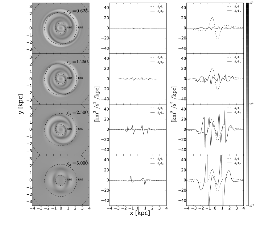
Figure 7: Results of a simulation in Wada’s potential in the case of a weak bar ($\epsilon=0.005$) for different values of the sound speed $c_{s}$. Each panel in the left column shows the steady-state density long after the bar has reached the final value of $\epsilon=0.005$ – compare with Fig. 4. The middle column shows the $y$ components of pressure forces (full lines) and bar perturbation gravitational forces (dashed line) from the potential in Eq. 13 with $\epsilon=0.005$ calculated along the horizontal axis. The right column shows the $x$ components of the same forces, again calculated along the horizontal axis. Note that pressure forces can be derived from a pressure potential $\Phi_{P}$ as described in the text.

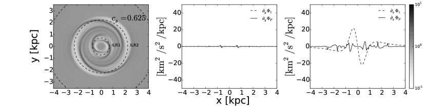
Figure 9: Same as the top row of Fig. 7, but for a simulation with twice the spatial resolution. Here, $\mathrm{d}x=10\,{\rm pc}$.

6 Strong Bar case

In the previous section, we have seen that in the weak bar case the spiral arms can be understood as kinematic density waves, generated by weakly oval closed orbits. What can we say about the strong bar case? In order to investigate a realistic example of a strong bar we consider a simulation we used in Sormani et al. (2015), performed in the Binney et al. (1991) barred potential. The simulation used here is the one with sound speed $c_{s}=10\,{\rm km\,s^{-1}}$ and spatial resolution $\mathrm{d}x=10\,{\rm pc}$.

In Sormani et al. (2015), spiral arms were present and noted, but not discussed in detail. It was shown that in the region where spiral arms are present the velocity field was very well approximated by $x_{1}$ orbits. To discuss the spiral arms, we will need to look at the tiny deviations of the hydro velocity field from the ballistic $x_{1}$ orbits field.

The left panel in Fig. 10 shows a density snapshot from the simulation in Sormani et al. (2015), taken after the bar is fully grown and the gas has reached an approximate steady state. Spiral arms emerging from the end of the bar are clearly identifiable. These spiral arms are stationary in the frame corotating with the bar. The central panel of Fig. 10 shows what happens when we nest together many instantaneous streamlines. We see that, to a very good approximation, streamlines are closed curves that when nested together generate the spiral arms. In the right panel ballistic closed orbits are shown for comparison. Fig. 11 analyses in more detail a selection of instantaneous streamlines in this snapshot. In the top panel, five streamlines are shown in dashed lines. These are very nearly closed. In the same panel, the ballistic closed orbits that cut the $y$ axis at the same value of the streamlines are shown in full lines. It can be seen that streamlines are librations around underlying closed $x_{1}$ orbits. In the middle panel, the same streamlines and orbits are shown in the $R\theta$ plane. In the bottom panel, the radial difference between the two orbits is shown in the $R\theta$ plane. The librations do not have the simple $\cos(2\theta)$ structure that we encountered in Sect. 5.

The above considerations strongly suggest that also in the strong bar case the spiral arms can be understood as kinematic density waves, generated by small librations around underlying closed orbits. In the epicycle approximation, the librations are around circular orbits. Here, the gas parcels librate around $x_{1}$ orbits. It is natural to ask whether the phenomenological models can be extended to the strong bar case, where now the perturbations should be made around the $x_{1}$ orbits and not around circular orbits. In order to investigate this, let us go back to the equations of motion in the rotating frame. For a gaseous parcel in a hydro simulation, Eq. (2) is modified to

$$\ddot{\mathbf{x}}=-\nabla(\Phi+\Phi_{P})+\Omega_{\rm p}^{2}\mathbf{x}-2\Omega_{\rm p}\left(\hat{\mathbf{e}}_{z}\times\dot{\mathbf{x}}\right)+F_{\mathrm{d}x}\;,$$ (27)

where $\Phi_{P}$ is the “potential” that gives the pressure force introduced above and $F_{\mathrm{d}x}$ is the viscous force. We can do a Floquet analysis to investigate librations around ballistic closed orbits (see for example Binney & Tremaine, 1987). Let us write $\Phi=\Phi_{0}+\Phi_{1}$, where this time $\Phi_{0}$ is not necessarily axisymmetric. Let $\mathbf{x}_{c}(t)$ be a ballistic closed orbit in the potential $\Phi_{0}$. We can write a libration around this closed orbit as $\mathbf{x}(t)=\mathbf{x}_{c}(t)+\mathbf{x}_{1}(t)$. By substituting this last equation into (27), expanding to first order in quantities with subscript 1 and cancelling the zeroth order terms, we obtain that the equation of motion for the libration is

$$\begin{split}\ddot{\mathbf{x}}_{1}&=-\left[(\mathbf{x}_{1}\cdot\nabla)\nabla\Phi_{0}+\nabla\Phi_{1}+\nabla\Phi_{P}\right]_{x_{c}(t)}+\Omega_{\rm p}^{2}\mathbf{x}_{1}\\ &\qquad-2\Omega_{\rm p}\left(\hat{\mathbf{e}}_{z}\times\dot{\mathbf{x}}_{1}\right)+F_{\mathrm{d}x}\;.\end{split}$$ (28)

In this equation, all the derivatives of the potentials are to be calculated along the unperturbed closed orbit and are therefore known functions of time. Equations (9) for the epicycle approximation can be considered as a particular case of Eq. (28), obtained assuming that $\Phi_{0}$ is axisymmetric, $\Phi_{P}=0$ and there are no viscosity forces (which are then added heuristically in the phenomenological models). In trying to generalise the analysis of Sect. 2 to the case when $\Phi$ is a strongly barred potential, we are faced with the difficulty that there is in general no natural way of splitting $\Phi$ into a $\Phi_{0}$ where we can easily calculate closed orbits and a perturbation $\Phi_{1}$ that only weakly deforms closed orbits. The only natural choice is to set $\Phi_{1}=0$. If this choice is made, the whole perturbing potential is given by $\Phi_{P}$, which is not known a priori. In the phenomenological models in the epicycle approximation we were able to neglect $\Phi_{P}$ compared to $\Phi_{1}$ in the low pressure case, but here the same cannot be done if $\Phi_{1}=0$.

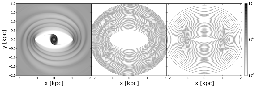
Figure 10: In the left panel, the density distribution for a simulation from SBM2015 with $c_{s}=10\,{\rm km\,s^{-1}}$ and spatial resolution $\mathrm{d}x=10\,{\rm pc}$. This snapshot is taken after the bar is fully grown and the final steady state is reached. The middle panel shows a nested sequence of instantaneous streamlines. The right panel shows ballistic closed $x_{1}$ orbits in the same underlying potential.

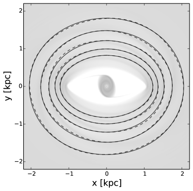
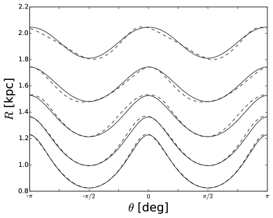
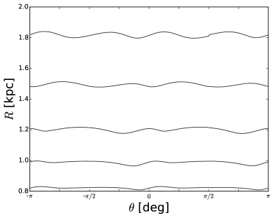
Figure 11: A Closer look at some of the streamlines of Fig. 10. In the top panel, streamlines (dashed lines) and ballistic $x_{1}$ orbits that cut the $y$ axis at the same value (full lines). In background is visible the density distribution of Fig. 10 for ease of comparison. The middle panel shows the same streamlines and orbits in the $R\theta$ plane. The bottom panel shows the difference $R_{\rm streamline}(\theta)-R_{x_{1}}(\theta)$, where the zero is shifted for clarity.

Suppose that $\Phi_{P}$ is somehow known. If we assume $\Phi_{1}=0$ and define a suitable phenomenological viscous term $F_{\mathrm{d}x}$ in Eq. (28), would the resulting equation correctly describe librations that give rise to spiral arms? To investigate this, we can do as follows. We first extract the density from the snapshot shown in the left panel of Fig. 10. From this density, we derive the pressure potential using Eq. (26) and $c_{s}=10\,{\rm km\,s^{-1}}$. Then we pretend we do not know how $\Phi_{P}$ was obtained and find librations using the following equation:

$$\boxed{\ddot{\mathbf{x}}_{1}=-\left[(\mathbf{x}_{1}\cdot\nabla)\nabla\Phi_{0}+\nabla\Phi_{P}\right]_{x_{c}(t)}+\Omega_{\rm p}^{2}\mathbf{x}_{1}-2\Omega_{\rm p}\left(\hat{\mathbf{e}}_{z}\times\dot{\mathbf{x}}_{1}\right)-2\lambda\dot{\mathbf{x}}_{1}}\;.$$ (29)

In this last equation, we have introduced a phenomenological dissipation term analogous to the models in the epicycle approximation. The dissipation is proportional to the difference between the total velocity and the local $x_{1}$ velocity field. $\Phi_{0}$, $\Phi_{P}$ and $\Omega_{\rm p}$ are now known, and given a value of $\lambda$ we can solve Eq. (29) to find the librations. Among all possible solutions to this equation, we want the solutions $\mathbf{x}_{1}(t)$ that are periodic with the same period of the underlying closed orbits. This amounts to finding the solution where transients are gone, dissipated away. The method that we used to solve the differential equation (29) is described in detail in Appendix A.

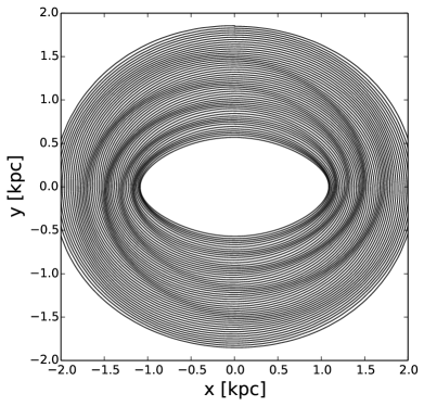
Figure 12: Nested librations around closed $x_{1}$ orbits generated using Eq. (29). The potential $\Phi_{0}$ is the potential used in SBM2015, the pressure potential $\Phi_{P}$ is derived from the density map in the left panel of 10, and $\lambda=50\,{\rm km\,s^{-1}}\,{\rm kpc}^{-1}$.

Fig. 12 shows a nested sequence of librations around $x_{1}$ orbits calculated using Eq. (29) and a value of $\lambda=50\,{\rm km\,s^{-1}}\,{\rm kpc}^{-1}$. Spiral arms identical to those present in the hydro simulation of Fig. (10) are recovered. This confirms that the spiral arms can be understood as kinematic density waves also in the strong bar case. Eq. (29) well describes the librations if the correct $\Phi_{P}$ is provided.

However, in the above analysis we have cheated in the sense that we have obtained $\Phi_{P}$ from the result a full hydrodynamical calculation. Is there a simple way of deriving a suitable $\Phi_{P}$, without solving the full hydrodynaical problem? We haven’t found a better way. We considered the possibility of obtaining $\Phi_{P}$ from the underlying closed orbits. Since the $x_{1}$ orbits are highly elongated, we have tried to infer a density map from orbit crowding, and from this the pressure potential. However, the pressure forces obtained in this way were much weaker than the one obtained in the hydro simulation for a value of the sound speed of $c_{s}=10\,{\rm km\,s^{-1}}$, and were not capable of reproducing spiral arms even for a small value of the dissipation. For a higher value of the sound speed we obtained segments of spiral arms that were not coherent and did not produce any “grand design”. Hence, we conclude that while the spiral arms in the strong bar case can still be explained by kinematic density waves generated by librations around the appropriate closed orbits, calculation of these librations require knowledge of the pressure forces and hence solution of the full hydrodynamical problem. Indeed, the morphology of the spiral arms found in Sormani et al. (2015) depends significantly on the value of pressure, and a phenomenological model that wants to reproduce must take pressure explicitly into account.

7 conclusion

In this paper, we have investigated bar-driven spiral arms in the absence of self-gravity. Our focus was on understanding the physical mechanism involved. We concluded that, both in the weak and strong bar cases, the spiral arms can be understood as kinematic density waves generated by librations around underlying ballistic closed orbits. In the weak bar case, the librations can be considered deviations from circular orbits. In the strong bar case, the librations are to be considered deviations from the appropriate underlying closed orbits, which can be highly elongated. In the strong bar case the epicycle approximation is not valid. In fact, whether a bar can be considered weak or strong is determined by the validity of the epicycle approximation. In Sect. 4 we argued that a bar is weak or strong according as the orbital structure is or is not obtainable from the epicycle approximation. Bars that might naively be considered weak, for example the case $\epsilon=0.05$, should be considered strong.

A parcel in a hydro simulation is subject to three different forces: gravitational, pressure and viscosity. We have tested the phenomenological models available in the literature aimed at explaining the spiral arms in the weak bar case, when the epicycle approximation is valid. We found that the key ingredient not taken into account by these models is pressure. Therefore they work well in regimes where pressure can be neglected, such as simulations in a weak bar at finite resolution and vanishing sound speed. We have also discussed how the phenomenological models should be extended to the strong bar case. When the pressure forces are known, these extensions work very well in explaining the spiral arms in the strong bar case. Unfortunately, the pressure forces are in general known only after solving the full hydrodynamical problem and are not known a priori. Thus, while the phenomenological models provide insight into the physical mechanism that generates the spiral arms, they appear to be of little practical use.

Appendix A Solving the Floquet Equation

In this Appendix we show how to solve Eq. (29). This equation arose during a Floquet analysis to find librations around closed orbits in a strongly barred potential. The equation to be solved is:

$$\ddot{\mathbf{x}}_{1}=-\left[(\mathbf{x}_{1}\cdot\nabla)\nabla\Phi_{0}+\nabla\Phi_{P}\right]_{x_{c}(t)}+\Omega_{p}^{2}\mathbf{x}_{1}-2\Omega_{p}\left(\hat{e}_{z}\times\dot{\mathbf{x}}_{1}\right)-2\lambda\dot{\mathbf{x}}\;.$$ (30)

Expanding into components, rearranging and renaming we can rewrite this equation as the following system:

$$\begin{split}\ddot{x}_{1}&=-x_{1}\kappa_{xx}(t)-y_{1}\kappa_{xy}(t)+F_{x}(t)+\Omega_{p}^{2}x_{1}-2\Omega_{p}\dot{y}_{1}-2\lambda\dot{x}_{1}\;,\\ \ddot{y}_{1}&=-x_{1}\kappa_{xy}(t)-y_{1}\kappa_{yy}(t)+F_{y}(t)+\Omega_{p}^{2}y_{1}+2\Omega_{p}\dot{x}_{1}-2\lambda\dot{y}_{1}\;,\end{split}$$ (31)

where

$$\begin{split}\kappa_{xx}(t)&=\left[\partial^{2}_{x}\Phi_{0}\right]_{x_{c}(t)}\;,\\ \kappa_{xy}(t)&=\left[\partial^{2}_{xy}\Phi_{0}\right]_{x_{c}(t)}\;,\\ \kappa_{yy}(t)&=\left[\partial^{2}_{y}\Phi_{0}\right]_{x_{c}(t)}\;,\\ F_{x}(t)&=-\left[\partial_{x}\Phi_{P}\right]_{x_{c}(t)}\;,\\ F_{y}(t)&=-\left[\partial_{y}\Phi_{P}\right]_{x_{c}(t)}\;.\end{split}$$ (32)

In Eqs. (31) it is assumed that $\lambda>0$ and that all the $\kappa$’s and $F$’s are given periodic functions of time with period $T$:

$$\begin{split}\kappa_{xx}(t)&=\kappa_{xx}(t+T)\;,\\ \kappa_{xy}(t)&=\kappa_{xy}(t+T)\;,\\ \kappa_{yy}(t)&=\kappa_{yy}(t+T)\;,\\ F_{x}(t)&=F_{x}(t+T)\;,\\ F_{y}(t)&=F_{y}(t+T)\;.\end{split}$$ (33)

The goal is to solve Eqs. (31) to find $\mathbf{x}_{1}(t)=\left(x_{1}(t),y_{1}(t)\right)$. We want to find the solution of this equation that neglects transients, i.e., the solution to which all solutions tend in the limit $t\to\infty$. This solution is the one such that $\mathbf{x}_{1}(t)$ is periodic with the same periodicity of the $F$’s and $k$’s. This is also a requirement if we want to obtain a closed orbit, and we have to assume such periodicity if our phenomenological model is to make sense. Let us therefore expand all time dependent quantities as Fourier series, assuming they are periodic with period $T$:

$$\begin{split}x_{1}(t)&=\sum_{n}X_{n}e^{in\omega t}\;,\\ y_{1}(t)&=\sum_{n}Y_{n}e^{in\omega t}\;,\\ \kappa_{xx}(t)&=\sum_{n}K_{xx;n}e^{in\omega t}\;,\\ \kappa_{xy}(t)&=\sum_{n}K_{xy;n}e^{in\omega t}\;,\\ \kappa_{yy}(t)&=\sum_{n}K_{yy;n}e^{in\omega t}\;,\\ F_{x}(t)&=\sum_{n}F_{x;n}e^{in\omega t}\;,\\ F_{y}(t)&=\sum_{n}F_{y;n}e^{in\omega t}\;.\end{split}$$ (35)

Fortunately, the product of the two Fourier series gives us another Fourier series of the same type. Substituting the Fourier expansions into Eqs. (31) and then equating coefficients term by term we arrive at

$$\begin{split}-\left[(n\omega)^{2}+\Omega_{p}^{2}\right]X_{n}&=\\ -\sum_{m}K_{xx;m}X_{n-m}&-\sum_{m}K_{xy;m}Y_{n-m}-(in\omega)\left[2\lambda X_{n}+2\Omega_{p}Y_{n}\right]+F_{x;n}\;,\\ -\left[(n\omega)^{2}+\Omega_{p}^{2}\right]Y_{n}&=\\ -\sum_{m}K_{yy;m}Y_{n-m}&-\sum_{m}K_{xy;m}X_{n-m}-(in\omega)\left[2\lambda Y_{n}-2\Omega_{p}X_{n}\right]+F_{y;n}\;.\end{split}$$ (36)

The last two equations are a linear algebraic system of equations in the unknowns $X_{n}$ and $Y_{n}$. All the other Fourier coefficients, $K$’s and $F$’s, are assumed to be known. To solve this system let us rewrite it in the form

$$\mathbb{A}\mathbf{X}=\mathbf{F}\;,$$ (37)

where $\mathbb{A}$ is an infinite matrix and

$$\mathbf{X}=\begin{pmatrix}\vdots\\ X_{-1}\\ Y_{-1}\\ X_{0}\\ Y_{0}\\ X_{1}\\ Y_{1}\\ \vdots\end{pmatrix}\;.$$ (38)

$\mathbf{F}$ is

$$\mathbf{F}=\begin{pmatrix}\vdots\\ F_{x;-1}\\ F_{y;-1}\\ F_{x;0}\\ F_{y;0}\\ F_{x;1}\\ F_{y;1}\\ \vdots\end{pmatrix}\;.$$ (39)

To write $\mathbb{A}$, let us divide it into a part $\mathbb{K}$ containing the Fourier coefficients of the $\kappa^{\prime}s$ and a part $\mathbb{D}$ that does not:

$$\mathbb{A}=\mathbb{D}+\mathbb{K}\;.$$ (40)

$\mathbb{D}$ is a block-diagonal matrix: it has $2\times 2$ blocks along the diagonal. Each block is

$$\mathbb{D}_{n}=\begin{pmatrix}-(n\omega)^{2}+2\lambda(in\omega)+\Omega_{p}&(in\omega)2\Omega_{p}\\ -(in\omega)2\Omega_{p}&-(n\omega)^{2}+2\lambda(in\omega)+\Omega_{p}\end{pmatrix}\;.$$ (41)

This is the block referring to the vector $(X_{n},Y_{n})$. The entire matrix $\mathbb{D}$ is then

$$\mathbb{D}=\begin{pmatrix}\ddots&&&&\\ &\mathbb{D}_{-1}&&&\\ &&\mathbb{D}_{0}&&\\ &&&\mathbb{D}_{1}&\\ &&&&\ddots\\ \end{pmatrix}\;.$$ (42)

The matrix $\mathbb{K}$ is

$$\mathbb{K}=\begin{pmatrix}\ddots&\vdots&\vdots&\vdots&\vdots&\vdots&\ddots\\ \cdots&\mathbb{K}_{0}&\mathbb{K}_{1}&\mathbb{K}_{2}&\mathbb{K}_{3}&\mathbb{K}_{4}&\cdots\\ \cdots&\mathbb{K}_{-1}&\mathbb{K}_{0}&\mathbb{K}_{1}&\mathbb{K}_{2}&\mathbb{K}_{3}&\cdots\\ \cdots&\mathbb{K}_{-2}&\mathbb{K}_{-1}&\mathbb{K}_{0}&\mathbb{K}_{1}&\mathbb{K}_{2}&\cdots\\ \cdots&\mathbb{K}_{-3}&\mathbb{K}_{-2}&\mathbb{K}_{-1}&\mathbb{K}_{0}&\mathbb{K}_{1}&\cdots\\ \cdots&\mathbb{K}_{-4}&\mathbb{K}_{-3}&\mathbb{K}_{-2}&\mathbb{K}_{-1}&\mathbb{K}_{0}&\cdots\\ \ddots&\vdots&\vdots&\vdots&\vdots&\vdots&\ddots\\ \end{pmatrix}\;,$$ (43)

where each $\mathbb{K}_{n}$ is a $2\times 2$ block given by

$$\mathbb{K}_{n}=\begin{pmatrix}K_{xx;n}&K_{xy;n}\\ K_{xy;n}&K_{yy;n}\end{pmatrix}\;.$$ (44)

Since the linear algebraic system represented by Eq. (37) is infinite, we need to truncate it in order to be able to solve it. On the diagonal of the matrix $\mathbb{K}$ there is $\mathbb{K}_{0}$. Suppose we truncate the Fourier expansion of all $\kappa$’s at order $\mathbb{K}_{0}$. Then the matrix $\mathbb{A}$ is block diagonal and the system is very easy to solve by considering only line pairs at a time. Now suppose we truncate the Fourier expansion of $\kappa(t)$ at some higher order. In this case, the matrix $\mathbf{A}$ is not block diagonal, but is a block band matrix that has elements on the sides of the diagonal up to the order of truncation. For example, if we truncate at $\mathbb{K}_{\pm 1}$, then we have a (block) band of width 3. To find the solution we need to truncate the system at some finite order and in general we cannot solve the system exactly as in the case in which we truncate at $\mathbb{K}_{0}$, where equations are decoupled in pairs. Thus there are two truncations involved. The first is where to truncate the Fourier expansions of $\kappa$ and $F$. This truncation has to be done at some order where $\kappa$ and $F$ are well represented by their Fourier expansions. The second is the size of truncation of the system $\mathbb{A}$, and must be done after the first truncation has been performed. This second truncation must be done for a size sufficiently high that the solution is converged and is not affected by a further increase in the size of the system. We have found that this convergence takes place quite rapidly.

References

- Athanassoula (1992) Athanassoula E., 1992, MNRAS, 259, 345
- Athanassoula et al. (2009a) Athanassoula E., Romero-Gómez M., Bosma A., Masdemont J. J., 2009a, MNRAS, 400, 1706
- Athanassoula et al. (2010) Athanassoula E., Romero-Gómez M., Bosma A., Masdemont J. J., 2010, MNRAS, 407, 1433
- Athanassoula et al. (2009b) Athanassoula E., Romero-Gómez M., Masdemont J. J., 2009b, MNRAS, 394, 67
- Binney et al. (1985) Binney J., Gerhard O. E., Hut P., 1985, MNRAS, 215, 59
- Binney et al. (1991) Binney J., Gerhard O. E., Stark A. A., Bally J., Uchida K. I., 1991, MNRAS, 252, 210
- Binney & Tremaine (1987) Binney J., Tremaine S., 1987, Galactic dynamics
- Binney & Tremaine (2008) Binney J., Tremaine S., 2008, Galactic Dynamics: Second Edition. Princeton University Press
- Bissantz et al. (2003) Bissantz N., Englmaier P., Gerhard O., 2003, MNRAS, 340, 949
- Contopoulos & Grosbol (1989) Contopoulos G., Grosbol P., 1989, Astronomy & Astrophysics Review, 1, 261
- Dame & Thaddeus (2008) Dame T. M., Thaddeus P., 2008, ApJ, 683, L143
- Dobbs & Baba (2014) Dobbs C., Baba J., 2014, Publications of the Astronomical Society of Australia, 31, 35
- Englmaier & Gerhard (1999) Englmaier P., Gerhard O., 1999, MNRAS, 304, 512
- Feldman & Lin (1973) Feldman S. I., Lin C. C., 1973, Studies in Applied Mathematics, 52, 1
- Huntley et al. (1978) Huntley J. M., Sanders R. H., Roberts, Jr. W. W., 1978, ApJ, 221, 521
- Lin & Lau (1975) Lin C. C., Lau Y. Y., 1975, SIAM Journal of Applied Mathematics, 29, 352
- Lin & Shu (1964) Lin C. C., Shu F. H., 1964, ApJ, 140, 646
- Lindblad & Lindblad (1994) Lindblad P. O., Lindblad P. A. B., 1994, in Astronomical Society of the Pacific Conference Series, Vol. 66, Physics of the Gaseous and Stellar Disks of the Galaxy, King I. R., ed., p. 29
- Piñol-Ferrer et al. (2012) Piñol-Ferrer N., Lindblad P. O., Fathi K., 2012, MNRAS, 421, 1089
- Rodriguez-Fernandez & Combes (2008) Rodriguez-Fernandez N. J., Combes F., 2008, A&A, 489, 115
- Romero-Gómez et al. (2007) Romero-Gómez M., Athanassoula E., Masdemont J. J., García-Gómez C., 2007, A&A, 472, 63
- Romero-Gómez et al. (2006) Romero-Gómez M., Masdemont J. J., Athanassoula E., García-Gómez C., 2006, A&A, 453, 39
- Sanders (1977) Sanders R. H., 1977, ApJ, 217, 916
- Sanders & Huntley (1976) Sanders R. H., Huntley J. M., 1976, ApJ, 209, 53
- Sormani et al. (2015) Sormani M. C., Binney J., Magorrian J., 2015, MNRAS, 449, 2421
- van Albada et al. (1982) van Albada G. D., van Leer B., Roberts, Jr. W. W., 1982, A&A, 108, 76
- Wada (1994) Wada K., 1994, Publications of the Astronomical Society of Japan, 46, 165
- Weiner & Sellwood (1999) Weiner B. J., Sellwood J. A., 1999, ApJ, 524, 112