Multi-GPU Graph Analytics

Abstract

We present a single-node, multi-GPU programmable graph processing library that allows programmers to easily extend single-GPU graph algorithms to achieve scalable performance on large graphs with billions of edges. Directly using the single-GPU implementations, our design only requires programmers to specify a few algorithm-dependent concerns, hiding most multi-GPU related implementation details. We analyze the theoretical and practical limits to scalability in the context of varying graph primitives and datasets. We describe several optimizations, such as direction optimizing traversal, and a just-enough memory allocation scheme, for better performance and smaller memory consumption. Compared to previous work, we achieve best-of-class performance across operations and datasets, including excellent strong and weak scalability on most primitives as we increase the number of GPUs in the system.

I Introduction

The potential advantages in performance, performance per dollar, and performance per watt of the modern graphics processing unit (GPU) over the traditional CPU [1] has led to a recent focus on GPU graph analytics [2, 3, 4, 5]. However, scalable GPU graph analytics frameworks today—those beyond one GPU—are still primarily in the research domain. In general, today’s GPU graph analytics frameworks, which we summarize in Section II-A, do not deliver both high performance and scalability while maintaining programmability and algorithm generality.

Single-GPU (“1GPU”) frameworks deliver excellent performance on graphs that fit into the GPU’s (limited) memory. Scaling to larger graphs and/or achieving higher performance require new approaches. We see three directions for scalability: multiple GPUs on a node (“mGPU”); the most common approach to date, multiple nodes (“mNode”); or leveraging the storage of a larger CPU memory (“out-of-core”). These directions are non-exclusive; future scalable systems may use more than one. Our performance results motivate our belief that mGPU graph processing should become the fundamental building block of GPU graph analytics.

Our work builds on our open-source “Gunrock” [5] graph-processing library for GPUs, whose programming model we summarize in Section II-B. While Gunrock previously targeted 1GPU and graphs that fit into 1GPU’s memory, we optimize and extend it in this work to mGPU. We believe that the conclusions we make in this paper will apply to other GPU graph frameworks as well.

To achieve high performance, scalability, programmability, and generality, we address several key questions:

• What is a general mGPU graph processing model?

• How to transform 1GPU programs to support mGPU?

• What data should be communicated, when, and how?

• How do we synchronize GPUs during computation?

• What is the indicator for convergence?

• What are the potential limiting factors to scalability?

• What are the optimizations for these limiting factors?

Addressing all of these goals is challenging. Supporting programmability and generality tends toward a high-level, flexible framework that abstracts away low-level details. However, performance and scalability concerns instead suggest low-level implementations that can efficiently leverage the underlying hardware. We also note other factors that can potentially limit performance and scalability: the type of graph partitioner used, the topology of the underlying graphs, and the necessary synchronization and communication patterns of each individual primitive.

Our work makes the following contributions:

1. Our mGPU graph processing library meets the above goals. Our framework allows programmers to easily extend 1GPU primitives to utilize mGPU’s capabilities.

2. We perform a detailed experimental analysis on potential limiting factors to scalability. We identify communication bandwidth; synchronization latency; efficient use of GPU memory; and partitioning strategy as the most significant obstacles. For partitioning strategy, we conclude that minimizing the size of partition borders as opposed to the traditional partitioners’ target of minimizing edge cuts is the right strategy for our system.

3. We design and implement generalized optimizations that effectively target these limiting factors, enhancing our performance and scalability. Our novel optimizations include efficient mGPU direction-optimizing traversal, and a just-enough memory allocation strategy that makes efficient use of GPU memory.

4. We achieve best-in-class performance on mGPU graph primitives, outperforming primitive-specific implementations on similar machine configurations. On 6 GPUs, we achieve more than 900 GTEPS (billion edges traversed per seconds) peak performance for direction-optimizing breath-first search (DOBFS) [6], and 2.63$\times$, 2.57$\times$, 2.00$\times$, 1.96$\times$, 3.86$\times$ geometric mean speedups as compared to 1GPU, and over various datasets for breadth-first search (BFS), single-source shortest path (SSSP), connected components (CC), betweenness centrality (BC) and PageRank (PR) respectively.

II Related Work

II-A Scalable GPU Graph Libraries

Numerous frameworks have targeted scalable graph analytics with multi-GPU approaches. We argue that in general, no previous multi-GPU work achieves our balance of high performance with programmability.

Merrill et al. [7] presented the first notable linear parallelization of the BFS algorithm on the GPU. Their 1GPU and mGPU implementations achieve excellent performance. In their mGPU implementation, vertices are distributed to GPUs, data related to remote vertices are fetched via peer memory access. Their approach only targets BFS, and adversely affects programmability by forcing programmers to handle cross-GPU data access within main computing steps. The peer memory access limits hardware compatibility, and also introduces load imbalance when accessing both local and remote vertices, which reduces performance.

The parallel BFS work by Fu et al. [3] extends the expand-contract BFS algorithm by Merrill et al. to GPU clusters. They propose a 2D partitioning method, and use MPI to contract columns on the edge frontiers after each expand step. The communication pattern limits data access within 1 hop, and thus restricts algorithm generality. Large edge frontiers transmitted between GPUs cause large communication overheads and limit scalability.

Bisson, Bernaschi, and Mastrofano [8] focused on building an mNode BFS implementation. They also utilize a 2D-partitioning scheme to reduce the amount of communication required. However, because of their use of costly atomic operations, their performance is limited.

Enterprise [9] is an mGPU work that targets BFS using BFS-specific optimizations. Their work achieves excellent performance on rmat graphs, but lacks the generality to target algorithms beyond BFS.

McLaughlin and Bader [10] targeted BC on GPU clusters, which distributed BFS work for different source vertices to different nodes. Its performance scales well in large part due to its novel use of task parallelism, but a task-parallel strategy is not applicable to most graph algorithms. Their framework also duplicates the graph across GPUs, limiting its scalability to graphs that can fit on 1GPU.

Medusa [2] was the pioneering mGPU graph library, taking a more general approach. It partitions the graph using Metis [11], makes replications for neighbor vertices within $n$ hops, and updates vertex-associated values every $n$ iterations. Their framework is limited in algorithm generality, because it cannot express algorithms that jump beyond the $n$-hop limit, such as Soman et al.’s CC algorithm [12]. Compared to its successors, it does not achieve top performance. And due to the data replication caused by a large number of vertices within $n$ hops of a partition boundary, their framework is not scalable in memory usage.

Totem [13] is a graph processing engine for GPU-CPU hybrid systems. It either processes the workload on the CPU or transmits it to the GPU according to a performance estimation model. This approach has the potential to solve the long-tail problem on GPUs, and overcome GPU memory size limitations. However, it has limitations in algorithm generality, because it can only work with algorithms that only access direct neighbors. Repeatedly moving data between CPUs and GPUs is costly, which makes scalability an issue.

Daga et al. [14] explored using an accelerated processing unit (APU, a single-chip CPU+GPU heterogeneous processor) to overcome the PCIe bandwidth limitation, but the APU’s memory bandwidth is significantly smaller than a discrete GPU, which hampers overall performance.

GraphReduce [15] is an out-of-core graph processing library for GPU. It uses a Gather-Apply-Scatter (GAS) framework, so it inherits GAS’s programmability and algorithm generality. Its out-of-core approach addresses the challenge of the GPU’s limited memory. However, it must stream the graph to the GPU during the computation, making the PCIe bus a performance bottleneck. Its use of only 1GPU also makes it unable to achieve performance scalability.

Frog [16, 17] differs from other frameworks here in requiring (expensive) preprocessing to color the graph into sets of independent vertices. With the colored graph, they can process colors asynchronously. However, performance is restricted by visiting all edges in each single iteration.

More recently, Groute [18] leveraged asynchronous computation to demonstrate impressive multi-GPU performance particularly on high-diameter, road-network-like graphs, and primitives that can benefit from prioritized data communication, such as SSSP and CC.

II-B Gunrock: GPU Graph Analytics

Our GPU-based graph analytics framework, Gunrock, targets both programmability and performance, and achieved them on 1GPU [5]. It proposes a data-centric programming model that presents graph primitives as a series of parallel graph operations on frontiers, which is a group of vertices or edges that are actively participating in the computation. It currently supports three ways to manipulate the frontier:

Advance

generates a new frontier by visiting the neighbors of the current frontier;

Filter

generates a new frontier by selecting a subset of the current frontier based on programmer-specified criteria;

Computation

executes an operation on all elements in the current frontier. This can be combined for efficiency with advance or filter.

Gunrock programs define graph algorithms as a sequence of the above three steps, beginning with an initial frontier and running to convergence.

III Our MGPU Graph Programming Abstraction

Our mGPU programming model is designed to balance programming complexity and performance. As much as possible, our philosophy is to enable programmers to specify algorithms at a high level, targeting a 1GPU implementation, while allowing our underlying mGPU framework to manage the necessary parallelization and communication details. Thus we make the following design decisions:

1. An mGPU implementation in our system uses a 1GPU primitive without modification; all mGPU machinery is transparent to it. This isolation not only simplifies the 1GPU to mGPU transformation, but also allows optimizations, either to primitives or to the underlying framework, to apply to both 1- and m-GPU cases.

2. To support mGPU primitives, programmers must specify the information listed in Section III-B.

3. Both because of GPU memory limitations and to leverage inter-GPU parallelism, our system partitions graphs across GPUs. We do not restrict the selection of the partitioner, leaving that decision to the programmer (Section V-C).

III-A Terminology

We define a graph $G(V,E)$ by its vertices $V$ and edges $E$, and its diameter as $D$. When partitioned, the $i^{th}$ GPU only holds a subgraph of $G$, denoted as $G_{i}(V_{i},E_{i})$, where $V_{i}$ and $E_{i}$ are the vertices and the edges stored on it. $B_{i,j}$ is the outgoing vertex border from GPU $i$ to GPU $j$, and $B_{i}$ is the union of all $B_{i,j}$, including duplications. We use $L_{i}$ to represent all vertices hosted by GPU $i$; $L_{i}$ may be a subset of $V_{i}$, because $V_{i}$ also contains remote proxy vertices (more in Section III-C). $n$ is the number of GPUs.

Because our system is bulk-synchronous across all GPUs, we use the BSP model [19] as a useful tool to analyze performance-limiting factors (Section V). In the BSP model, $W$ is the cost of local computation on a single node (analyzed in Section IV); $H$ is the number of messages transmitted (communication volume, the size of data transmitted between GPUs); $g$ is the time to deliver a single message under continuous traffic conditions (we use the inverse of inter-GPU communication bandwidth); $S$ is the number of supersteps (iterations); and $l$ is the synchronization cost (per-iteration overhead). We use $C$ to represent the cost of communication computation, which is the computation required to facilitate inter-GPU communications.

III-B Extending 1GPU Programs to mGPU

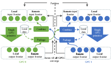
Figure 1: mGPU Framework highlighting communications

Our mGPU framework is illustrated in Fig. 1. The core of an mGPU primitive is an unmodified 1GPU primitive, which we extend to mGPUs by using the iteration synchronization point to exchange data between GPUs. By making our mGPU framework transparent to 1GPU primitives, we separate the concerns of per-GPU computation and inter-GPU communication: as long as the input frontiers for each iteration are prepared correctly, and the per-vertex associative values are updated properly before they are used in the next iteration, a core graph primitive does not need to know whether a vertex is hosted on a local or remote GPU.

At the end of an iteration, a 1GPU primitive concludes its computation and globally synchronizes before beginning the next iteration. At that point, our framework takes over, performing the following steps: it splits the output frontier of vertices into local and remote sub-frontiers, then packages the remote sub-frontier with its primitive-specific associated data, identified by the programmers, such as labels or predecessor vertex ids, and pushes the packaged data to peer GPUs. When a GPU receives data, our framework combines that data with that GPU’s local data, and (if necessary) also adds the received vertices into its input frontier for the next iteration. A GPU that hosts vertex $V$ may receive updates to $V$ from multiple remote GPUs. It must combine those updates into a single value for $V$. The programmer specifies how that combining must be done—for instance, taking the minimum value from all updates, as in BFS or SSSP—but the framework will actually perform the combining.

Our mGPU framework also initializes the computation by partitioning the graph and its associated per-{vertex, edge} data, reordering or relabeling if necessary, distributing all data to the correct GPUs, and initializing the starting frontier.

Programmers must specify the following information:

Core single-GPU primitive

Use Gunrock operators to define a series of operations on input frontiers.

Data to communicate

What kinds of data associated with vertices must be pushed to remote GPUs? We have not seen primitives that require per-edge communication between GPUs, and argue that any such primitive will scale poorly based on the large volume and computation workload required by per-edge communication.

Combining remote and local data

Specify the operation to combine local and (possibly multiple) received data at the beginning of an iteration, except the first one.

Stop condition

Define the local and/or global stop condition so that each local GPU will properly exit its computing iteration when the algorithm finishes.

and the framework handles all other aspects:

Split frontier

Split the output frontier of an iteration into local and remote sub-frontiers.

Package data

Package the remote sub-frontiers with the associated data that specified by the programmer. Data packaging can be done together with frontier splitting.

Push to remote GPUs

Manage communication so that each GPU pushes the right information to the right GPU for use in the next iteration.

Merge local and received sub-frontiers

Using the combiner specified by the programmer, efficiently merge the local sub-frontier with all received sub-frontiers to get the input frontier for the next iteration.

Manage GPUs

Our framework manages each GPU by a dedicated CPU thread to avoid false dependencies between GPUs. It also uses multiple GPU streams on a GPU to overlap computation and communication, by separating them into different streams. We synchronize and establish dependencies between GPUs without CPU intervention by using cudaStreamWaitEvent().

III-C Vertex Duplication and Communication Strategy

We partition the graph (Section V-C) as a pre-processing stage, and currently support partitioners that do edge cuts, i.e., vertices are distributed to individual GPUs, together with their outgoing edges. To isolate the computation to local data only, remote vertices need to be duplicated locally. We implemented two strategies for this duplication:

Duplicate-1-hop:

create a local proxy vertex only for the immediate remote neighbors of $L_{i}$ on GPU_i; vertices in $V_{i}$ are renumbered with continuous IDs.

Duplicate-all:

create a local proxy vertex for every remote vertex, i.e., force $V_{i}$ to be $V$. We still distribute $E$, so remote vertices in $V_{i}$ have 0 outgoing edges on GPU $i$.

We also implemented two strategies for communication:

Broadcast:

in each iteration, each GPU broadcasts the whole generated frontier to all other GPUs.

Selective-communicate:

we send frontier vertices to only their hosting GPUs or to the GPUs that host their proxies. This requires a splitting step on the vertex frontier to assemble a separate sub-frontier of vertices to each remote GPU.

The programmer can choose the strategies. Duplicate-1-hop uses less memory space, but requires ID conversion for communication; on the other hand, duplicate-all requires no ID conversion but uses more memory. Broadcasting saves the work required to split the frontier, but consumes more memory and communication bandwidth, and introduces a higher computation workload when combining received data. Selective communication requires less memory and communication bandwidth, but it cannot bypass the splitting step. If an algorithm only needs to access the immediate neighbors of incoming or outgoing edges, then duplicate-1-hop and selective-communication are better choices; otherwise, algorithms that access both incoming and outgoing neighbors (e.g., DOBFS), or that visit vertices with more than one hop distance (e.g., CC), require broadcasting, and usually use the duplicate-all strategy.

IV Algorithms in Our Abstraction

Primitive	Computation ($W$)	Communication Computation ($C$)	Communication Volume ($H$)	Iterations ($S$)
BFS	$O(|E_{i}|)$	$O(|V_{i}|)$	$O(|B_{i}|)$	$\sim D/2$
DOBFS	$O(a\times|E_{i}|)$	$O(|V|)$	$O((n-1)\times|V|)$	$\sim D/2$
SSSP	$O(b\times|E_{i}|)$	$O(b\times|V_{i}|)$	$O(2b\times|B_{i}|)$	$\sim b\times D/2$
BC	$O(2\times|E_{i}|)$	$O(2\times|V_{i}|+|V|)$	$O(5|B_{i}|+2(n-1)\times|L_{i}|)$	$\sim D/2$
CC	$\log(D/2)\times O(|E_{i}|)$	$S\times O(|V_{i}|)$	$S\times O(2|V_{i}|)$	2–5
PR	$S\times O(|E_{i}|)$	$S\times O(|B_{i}|)$	$S\times O(|B_{i}|)$	data-dependent

TABLE I: Summary of Algorithms. Terminology is summarized in Section III-A.

We implemented six graph primitives with our framework, several of which are straightforward extensions (from the programmer’s perspective) from 1GPU implementations. Included in Appendix A is an example BFS implementation using the mGPU framework, with programmer provided blocks highlighted. Because DOBFS has different runtime and communication properties, and thus different scaling behavior, we consider it as a separate algorithm in our scalability analysis. SSSP and BC have similar scaling properties to BFS, while CC and PR are both non-traversal primitives that operate on all vertices and all edges of the graph. We thus select DOBFS, BFS, and PR as representative primitives for further analysis, and summarize all six algorithms in Table I. Except for DOBFS and for graphs that have too little computation to fill the GPU on an iteration, most primitives are bounded by computation.

  Algorithm 1 Multi-GPU BFS

 

1:Vertex duplication: Duplicate-all. We trade memory usage for better performance for BFS.

2:Computation: An advance kernel followed by a filter kernel, as introduced by Merrill et al. [7]. $W{\in}O(|E_{i}|)$.

3:Communication: Selective-communicate. Only the remote vertices are sent.

4:Combination: If a received vertex has not been visited before, update its label and place it in the input frontier on the next iteration. $H{\in}O(|B_{i}|)$, and $C{\in}O(|V_{i}|)$.

5:Convergence: All frontiers are empty. $S{\approx}D/2$.

 

  Algorithm 2 Multi-GPU DOBFS

 

Vertex duplication: Duplicate-all. It couples better with the broadcast communication strategy.

2:Computation: Summarized in Section VI-A. For graphs with high average out-degrees, $W{\in}O(|L_{i}|)$; for other graphs in practice, $W{\in}O(a\times|E_{i}|)$ where $a<1$.

Communication: Broadcast, because an upcoming iteration may use either the forward or backward direction.

4:Combination: Same as BFS. $H{\in}O(|V|)$ and $C{\in}O((n-1)|V|)$.

Convergence: Same as BFS. $S{\approx}D/2$.

 

  Algorithm 3 Multi-GPU PR

 

Vertex duplication: Either duplicate-all or duplicate-1-hop. The remote sub-frontiers do not change over iterations. We get all these sub-frontiers during the initialization step, and only send ranking values during actual computation. There is no significant performance or memory usage difference between these two, and we use duplicate-all to better trace the program.

Computation: A filter kernel updating the PR values (except 1^st iteration), followed by an advance kernel accumulating the PR values for each vertex. $W{\in}O(|E_{i}|)$.

3:Communication: Selective-communicate. Push locally accumulated ranks of each vertex to its hosting GPU.

Combination: Do an atomicAdd to combine received rank with the local copy. $H{\in}O(|B_{i}|)$ and $C{\in}O(|B_{i}|)$.

Convergence: Terminates when all ranking value updates are smaller than a pre-defined threshold ratio, or a given maximum number of iterations is reached. $S$ does not affect the scalability.

 

V Performance Limiting Factor Analysis

In this section we describe and analyze potential performance bottlenecks for our mGPU implementation that are specific to graph computation and mGPU systems. The BSP computation model [19] states that the total computation cost of a parallel program can be expressed as $W+Hg+Sl$.

V-A Communication

The inter-GPU bandwidth $1/g$ is determined by the system. Certainly any mGPU system should enable the highest-bandwidth connection. For instance, enabling peer GPU-GPU communication on our system (K40s on the same PCIe3 root hub) increases GPU-GPU bandwidth from $\sim$16 GB/s to $\sim$20 GB/s with a corresponding latency decrease from $\sim$25 us to $\sim$7.5 us.

What software can affect is the communication volume $H$. $H$ is perhaps the most important factor in scaling for a given primitive. We list $H$ for individual primitives in Table I. To get a clearer idea how $H$ affects the performance, we artificially increased it and found that in general, runtime varies linearly with the increase of $H$. We also found that increasing $H$ affects DOBFS more than BFS and PR, because $W$ and $H$ of DOBFS are close in scale, especially when running on rmat graphs (both are roughly in $O(|V|)$), whereas $W$ is larger than $H$ for BFS and PR. Datasets with high vertex counts suffered more from $H$ increases. Another possible factor that may influence performance is communication latency, but it’s only a small portion of $l$, and even when we artificially increase it by a factor of ten, we see no appreciable difference in performance.

V-B Synchronization

The per-iteration synchronization latency $l$ includes the effects of kernel launch overheads ($\sim$3 $\mathrm{\SIUnitSymbolMicro s}$ per kernel) during primitive computation, load imbalance between GPUs, and API and kernel launching overheads of the communication-computation kernels. In our experiments, $l$ is significant when the other parts run in the sub-$\mathrm{\SIUnitSymbolMicro s}$ range or $S$ is large.

The GPU also needs a large workload to maintain high processing rates [20]. If per-GPU workloads aren’t large enough, kernel launch overheads also occupy a large portion of the total running time. Traversal on road networks is one example that suffers from both launch latency and GPU under-utilization; one iteration of even a large road network traversal doesn’t have enough work to keep even 1GPU busy. We also see this overhead when processing, for instance, DOBFS on rmat, where many iterations only take a few $\mathrm{\SIUnitSymbolMicro s}$.

To study the effect of $l$, we let each GPU visit only 1 vertex and 1 edge in each iteration. This is the smallest per-iteration workload possible, and the BFS running time on it can be used as an measurement of $l$. The running time is linear with $S$, and the average per-iteration time for large $S$ for {1,2,3,4} GPUs is {66.8, 124, 142, 188} $\mathrm{\SIUnitSymbolMicro s}$. The jump from one to two GPUs reflects the effect of inter-GPU synchronization and communication latency.

V-C Partitioner

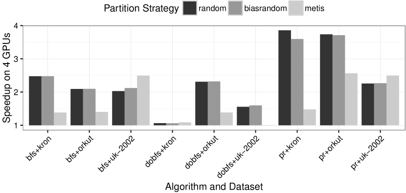
Figure 2: Performance impact of partitioners on 3 primitives $\times$ 3 datasets.

We recognize that good partitioners can help increase mGPU graph processing performance. Most partitioners attempt to minimize the number of edges cut across partitions. However, in our system, it is instead the size of partition borders ($B_{i}$, the number of vertices on partition edges, as summarized in Table I) that is most important to our performance. This is because our framework communicates values associated with vertices, and multiple cut edges from the same GPU that point to the same remote vertex only need to transmit one set of values regarding that vertex.

To gain insight into partitioner behavior, we use three different partitioners, listed in increasing order of partitioner runtime: random (randomly assign vertices to GPUs), biased random (like random, but biased toward assigning a vertex to a GPU that contains more of its neighbors), and Metis [11]. We summarize their effects in Fig. 2. While the random partitioner captures no graph locality, it does achieve excellent load balancing, and performs fairly well across our tests. Biased random tries to reduce the border size without affecting the load balancing too much, and shows performance very close to the random partitioner. Metis only wins in a few situations, with small margins, but takes a much longer time to partition. With this in mind, all other experiments in this paper use the random partitioner. Without ideal partitioner candidates, we chose to make our partitioner interface modular and allow users to specify any existing partitioner or implement their own; we ensure that the framework and primitives will run correctly regardless of the choice of partitioner.

VI Optimizations

With 1GPU Gunrock, we begin with a framework that already has numerous optimizations for good performance. We add several more to specifically address mGPU operation and the performance-limiting factors from Section V.

VI-A Direction-optimizing Traversal

Traditional BFS performs a forward (“push”) traversal where vertices in the current frontier add their unvisited neighbors to the output frontier. Beamer et al.’s DOBFS [6] adds the ability to perform a backward (“pull”) traversal, beginning from a frontier of all unvisited vertices, to visit parent vertices. If one of those parent vertices is in the current frontier, visiting all other edges can be skipped. This “edge skipping” can significantly improve BFS performance for small-diameter graphs, but mapping existing implementations to a distributed context is a challenge.

Beamer et al. implemented this operation by scanning all vertices and processing the unvisited ones. This is inefficient, and introduces load imbalance between visited and unvisited vertices. Our previous 1GPU implementation had two deficiencies when parallelized across GPUs.

First, our 1GPU advance kernel parallelizes across edges and thus cannot efficiently skip edges once a parent is found. We added an advance mode that parallelizes across vertices, thus serializing edge visits and allowing us to stop work when we discover a valid parent. We then split the unvisited vertex frontier from the previous iteration into two parts, newly-discovered vertices and unvisited vertices. The newly discovered vertex frontier is important for our mGPU implementation, because it gives a direction-independent view for the framework (advances in both directions output the newly discovered vertices), and also a cost-free transformation from backward to forward.

Second, the traditional DOBFS computation for switching between push and pull would require additional computation (potentially of the same scale of the actual traversal) to get the number of edges needed to visit in the next iteration. We change the direction-selection condition to only require inputs that are already available. Let $Q$ be the current frontier and $U$ and $P$ the unvisited and visited vertices. We can estimate the number of forward edges visited as $FV=\frac{|Q|\cdot|E_{i}|}{|V_{i}|}$ and the number of backward edges visited as $BV=\frac{|U|\cdot|V_{i}|}{|P|}$. We begin with forward traversal; then at the beginning of each subsequent iteration, if we see that $FV>BV\cdot do\_a$, we switch from forward to backward; if $FV<BV\cdot do\_b$, we switch from backward to forward. Because every time we switch from forward to backward, we must scan all vertices for unvisited ones, we only allow this switch once. The optimal values of $do\_a$ and $do\_b$ for similar graph types appear to be consistent; for example, $do\_a=0.01$ and $do\_b=0.1$ gives good performance for social graphs. We found these parameters are mostly mGPU-independent, i.e., the same set of parameters can be used for different numbers of GPUs.

These optimizations permit a significantly more efficient mGPU DOBFS, one that outperforms previous BFS and DOBFS implementations by a significant margin, but also uncovers a more fundamental bottleneck. DOBFS’s principal computation advantage is effectively reducing $W$ to $O(a\cdot|E_{i}|)$, where $a$ is less than 1. For graphs where $|E_{i}|{\gg}|V_{i}|$, such as rmat graphs with large edge factors, $W$ reduces to $O(|V_{i}|)$. But because the upcoming iteration may use either direction, which essentially requires sending the newly discovered frontiers to all peers (i.e., broadcast), $H$ and $C$ thus increase to $O(|V|)$, which can be on par with $W$. The result is an implementation that is primarily bound by communication with flat strong and weak scaling behavior (Section 4). Reducing communication cost is the priority for future mGPU DOBFS implementations.

VI-B Just-enough Memory Allocation

Figure 3: Memory consumption using different allocation schemes on kron, soc-orkut, and uk-2002 running BFS. Details of the schemes are described in Section VI-B.

Because GPU memory capacity is limited, it is crucial to use it efficiently, particularly for large graphs. What makes this challenging is that iterative graph primitives usually produce frontiers with a size that is unknown until the finish of an advance or filter kernel. One option is to allocate memory that is large enough to handle any case, e.g., a size $|E|$ array for advance. However, this maximum allocation artificially limits the size of the subgraph we can place onto one GPU, which either (a) requires us to use more GPUs to solve a particular problem or (b) limits our scalability to less than we could potentially achieve.

Instead of worst-case allocation, we implement a just-enough memory allocation scheme to use our memory more efficiently. We make a reasonable estimate of memory allocation before computation and then reallocate if this allocation is insufficient. In practice, our “reasonable” estimates are usually sufficient so reallocation, which is expensive, is infrequent. We mainly reallocate before advance, filter, or communicate operations. For advance, we leverage Gunrock’s load-balancing computations to correctly compute output size or add an extra reduction to determine output size. For filter, the output size is at most the size of input, and for most filters, the output size is capped by $|V_{i}|$. For communication, the required size is given by the framework.

We compare just-enough memory allocation against 3 alternatives (Fig. 3): a fixed preallocation using sizing factors calculated from previous runs of similar graphs; a maximum allocation; and preallocation plus kernel fusion (in Section VI-C). The just-enough memory allocation is still in effect when these alternatives are used, to prevent illegal memory access, although this only happens rarely. Each of the different memory allocation schemes have near-identical computation times. Just-enough allocation is critical in reducing our memory footprint, which allows us to fit larger subgraphs into memory. Consequently, we can achieve higher performance with fewer GPUs than other frameworks that lack sophisticated memory management strategies (Section VII-C). Our implementation of (DO)BFS, SSSP and BC use preallocation plus kernel fusion (Section VI-C); we use fixed preallocation for CC and PR, as their memory requirements can be determined before running these primitives.

VI-C Kernel Fusion

Kernel fusion (automatically combining two sequential kernels into one) is a well-known technique for high-performance GPU graph analytics [7, 20]. Our previous 1GPU work [5] fused Gunrock compute operators with advance or filter operators. In this work we added the ability to fuse an advance operator with a filter operator that follows it. In addition to the usual advantages of reducing kernel launch overhead and increasing producer-consumer locality, this particular fusing eliminates the need to store the intermediate frontier (potentially as large as $O(|E|)$) in GPU memory, enabling us to store larger subgraphs per GPU.

VII Results

We begin by summarizing the results that we present in more detail later in this section.

• Primitives in our framework scale reasonably well from 1 to 6 GPUs (geometric mean of speedup: 2.52$\times$ across five primitives), except for DOBFS, whose scalability is limited by communication overhead.

• (DO)BFS and PR show good weak scaling. BFS and PR exhibit strong scaling, but DOBFS does not.

• We compared our performance against previously-published in-core multi-GPU systems on the datasets highlighted by those systems. In general, we significantly outperform other systems given the same number of GPUs, and often systems with many more GPUs.

VII-A Experimental Setup

group	name	$|V|$	$|E|$	$D$	group	name	$|V|$	$|E|$	$D$	group	name	$|V|$	$|E|$	$D$
soc	soc-LiveJournal1	4.85M	85.7M	13	web	indochina-2004	7.41M	302M	24	rmat	rmat_n20_512	1.05M	728M	6.26∗
soc	hollywood-2009	1.14M	113M	8	web	uk-2002	18.5M	524M	25	rmat	rmat_n21_256	2.10M	839M	7.22∗
soc	soc-orkut	3.00M	213M	7	web	arabic-2005	22.7M	1.11B	28	rmat	rmat_n22_128	4.19M	925M	7.56∗
soc	soc-sinaweibo	58.7M	523M	5	web	uk-2005	39.5M	1.57B	23	rmat	rmat_n23_64	8.39M	985M	8.32∗
soc	soc-twitter-2010	21.3M	530M	15	web	webbase-2001	118M	1.71B	379	rmat	rmat_n24_32	16.8M	1.02B	8.61∗
										rmat	rmat_n25_16	33.6M	1.05B	9.06∗

TABLE II: Datasets we used to evaluate our work. $|V|$ and $|E|$ are vertex and edge counts; $d$ is the graph diameter, ^∗ indicates an approximated diameter computed by multiple run of random-sourced BFS.

We run most tests on nodes with 6 NVIDIA Tesla K40 cards, a 10-core Intel Xeon E5-2690 v2, and 128 GB CPU memory, running on CentOS 6.6 with CUDA 7.5 (both driver and runtime) and gcc 4.8.4. We conduct strong and weak scaling experiments on 2 systems: (1) 4 NVIDIA Tesla K80 cards (each with 2 GPUs and 12 GB DRAM/GPU) and (2) 4 Tesla P100s (PCIe, 16 GB DRAM, CUDA 8.0). Direct peer-to-peer inter-GPU communication is enabled in groups of 4 GPUs where appropriate. All programs are compiled with the -O3 flag and set to target the actual streaming multiprocessor generation of the GPU hardware.

The dataset information is listed in Table II in three representative groups. The real-world graphs are from the UF sparse matrix collection [21] and the Network Data Repository [22]. The “soc” and “web” groups are online social networks and web crawls of different domains. For SSSP, edge values are randomly generated integers from [0, 64]. We implement a GPU-based R-MAT “rmat” graph generator faithful to GTgraph [23]; the rmat parameters are {A, B, C, D} = {0.57, 0.19, 0.19, 0.05}. All three kinds of graphs follow a power-law distribution. Road networks, and high-diameter, low-degree graphs in general, have very different scalability characteristics than power-law graphs. They have insufficient parallelism to saturate even 1GPU, much less mGPUs; as a result, iteration overhead occupies a significant portion of the runtime, and we observed performance decreases on mGPU. If otherwise unspecified, all graphs we use are converted to undirected graphs. Self-loops and duplicated edges are removed. All tests have been repeated at least 10 times with average runtime used for results. Computations are verified for correctness. The instructions and the scripts to reproduce the results can be found at https://github.com/gunrock/gunrock/tree/master/dataset/test-scripts/ipdps17.

VII-B Overall Results

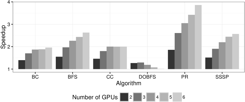
Figure 4: mGPU speedup over 1GPU performance for BC, BFS, CC, DOBFS, PR and SSSP. All numbers shown are geometric means of runtime speedup over all datasets.

The overall speedup of all the primitives is shown in Fig. 4, normalized to the performance of 1GPU as 1. The speedup of a given primitive using a given number of GPUs is the geometric mean of speedups from all datasets tested for that configuration. Most of the primitives scale well from 1 to 6 GPUs, resulting in 2.63$\times$, 2.57$\times$, 2.00$\times$, 1.96$\times$ and 3.86$\times$ speedup for BFS, SSSP, CC, BC and PR respectively using 6 (K40) GPUs. The performance curve of DOBFS mostly stays flat, as it’s limited by communication overhead. This agrees with our scaling analysis in Section V and  VI-A.

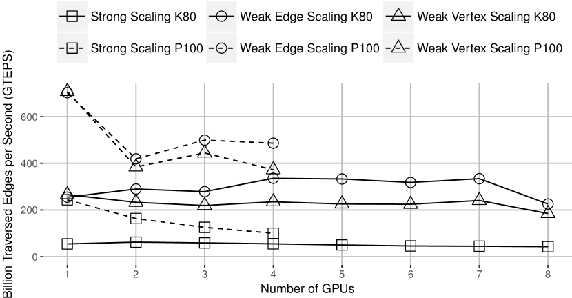
(a) DOBFS scalability

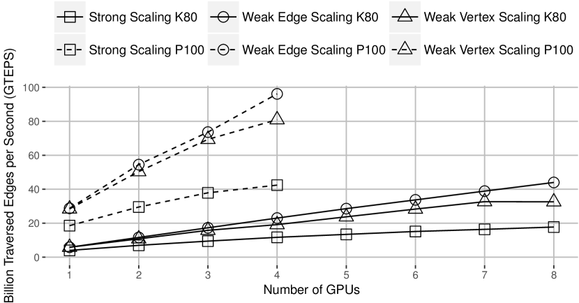
(b) BFS scalability

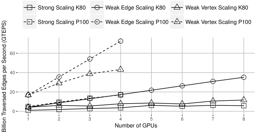
(c) PR scalability

Figure 5: Scalability of DOBFS, BFS, and PR. {Strong, weak edge, weak vertex} scaling use rmat graphs with {$2^{24}$, $2^{19}$, $2^{19}\times|\text{GPUs}|$} vertices and edge factor {32, 256$\times|\text{GPUs}|$, 256} respectively.

As in Section IV, we focus on (DO)BFS and PR as representative primitives for further analysis. Fig. 5 shows strong and weak scaling of these selected primitives. While providing both weak-vertex and -edge scaling, DOBFS doesn’t have good strong scaling, because its computation and communication are both roughly in the order of $O(|V_{i}|)$. This effect is more obvious on P100, as computation is faster but inter-GPU bandwidth stays mostly the same. As a result, the peak BFS performance (513 GTEPS on K40, and 900 GTEPS on P100) is achieved by 1GPU DOBFS with rmat_n20_512. In contrast, BFS and PR achieve almost linear weak and strong scaling from 1 to 8 GPUs.

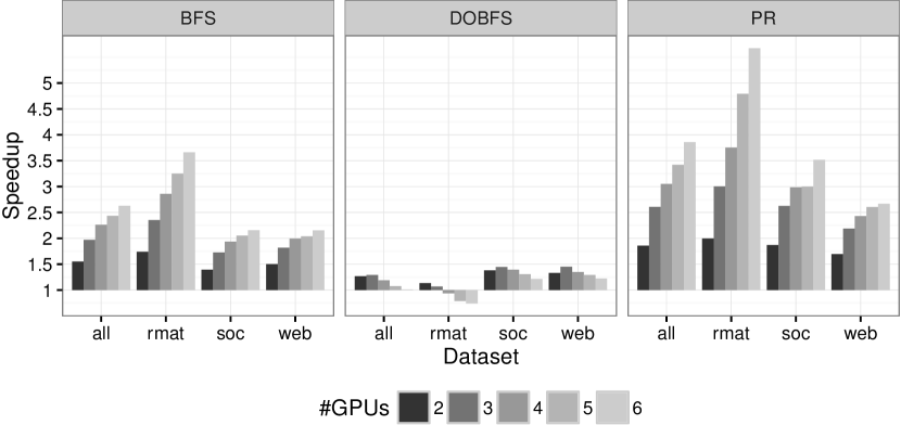
Figure 6: mGPU geometric mean speedups over 1GPU performance on rmat, soc and web graphs separately and in geometric means (all) for DOBFS, BFS, and PR.

We show more detailed speedups separated by graph type in Fig. 6. DOBFS scaling suffers the most for rmat datasets, because the volume and computation for communication vs. the core computation complexity is higher, resulting in a correspondingly larger portion of per-iteration time for inter-GPU communications. On the other hand, the larger $|E_{i}|/|V_{i}|$ ratio of rmat graphs helps BFS and PR in scalability, because the core computation cost is $O(|E_{i}|)$ and the communication cost is at most $O(|V_{i}|)$, reducing the cost of communication compared to computation.

VII-C Comparisons vs. Previous mGPU Work

graph	ref.	ref. hw.	ref. perf.	our hw.	our perf.	comp.
kron_n24_32 (16.8M, 1.07B, UD)	Liu [9]	{2, 4}$\times$K40$\times$1	{15, 18} GTEPS	{2, 4}$\times$K40	{77.7, 67.7} GTEPS	{5.18, 3.76}$\times$
kron_n24_32 (16.8M, 1.07B UD)	Liu [9]	8$\times$K40$\times$1	18.4 GTEPS	4$\times$K80	40.2 GTEPS	2.18$\times$
rmat_2Mv_128Me (2M, 128M, D)	Merrill [7]	4$\times$K40$\times$1N	11.2 GTEPS	4$\times$K40	29.9 GTEPS	2.67$\times$
coPapersCiteseer (0.43M, 32.1M, UD)	Zhong [2]	4$\times$C2050$\times$1E	2.69 GTEPS	4$\times$K40	3.31 GTEPS	1.23$\times$
com-orkut (3M, 117M, UD)	Bisson [8]	1$\times$K20X$\times$4	2.67 GTEPS	4$\times$K40	14.22 GTEPS	5.33$\times$ $|$ 4.62$\times^{*}$
com-Friendster (66M, 1.81B, UD)	Bisson [8]	1$\times$K20X$\times$64	15.68 GTEPS	4$\times$K40	14.1 GTEPS	0.90$\times$ $|$ 0.78$\times^{*}$
kron_n23_16 (8M, 256M, UD)	Bernaschi [24]	1$\times$K20X$\times$4	$\sim$1.3 GTEPS	4$\times$K40	30.8 GTEPS	23.7$\times$ $|$ 20.6$\times^{*}$
kron_n25_16 (32M, 1.07B, UD)	Bernaschi [24]	1$\times$K20X$\times$16	$\sim$3.2 GTEPS	6$\times$K40	31.0 GTEPS	9.69$\times$ $|$ 8.41$\times^{*}$
kron_n25_32 (32M, 1.07B, D)	Fu [25]	2$\times$K20$\times$32	22.7 GTEPS	4$\times$K40	32.0 GTEPS	1.41$\times$ $|$ 1.02$\times^{*}$
kron_n23_32 (8M, 256M, D)	Fu [25]	2$\times$K20$\times$2	6.3 GTEPS	4$\times$K40	27.9 GTEPS	4.43$\times$ $|$ 3.20$\times^{*}$
twitter-mpi (52.6M, 1.96B, D)	Bebee [26]	1$\times$K40$\times$16	224.2 ms	3$\times$K40	94.31 ms	2.38$\times$

TABLE III: Comparison with previous in-core GPU BFS work. Ref. hardware is denoted by intra-node GPU count$\times$GPU model$\times$node count. We use the same number of GPUs whenever possible within the constraints of a single node. $*$ indicates speedup adjustment by memory bandwidth ratio, $N$ indicates results reproduced on our system, and $E$ indicates issues in reproducing results; refer to Section VII-C for details.

graph	algo	ref.	ref. perf.	our hw.	our perf.
uk-2002	{BFS, SSSP, CC, PR}	Sengupta [15], 1$\times$K40E	{49, 80, 153, 162} sec	1$\times$K40	{0.059, 0.76, 1.85, 1.99} sec
twitter-rv	{BFS, SSSP, CC, PR}	Shi [17], 1$\times$K40N	{46, 40‡, 29, 80} sec	{1, 2, 3, 1}$\times$K40	{0.098, 0.837‡, 1.71, 49.7} sec
LiveJournal1	{BFS, SSSP, CC, PR}	Shi [16], 1$\times$K40N	{66.4, 245‡, 213, 105} ms	1$\times$K40	{12.2, 63.2‡, 93.6, 45.7} ms
twitter-rv	{SSSP, CC, PR}	Lee [27], 4 cores$\times$21 nodes	{126, 304, 149} sec	{2, 3, 1}$\times$K40	{2.20, 1.71, 49.7} sec
twitter-mpi	{BFS, SSSP, BC, PR}	Gharaibeh [13], 2$\times$ K40+2$\times$Xeon 2637N	{0.698, 2.67, 3.90, 0.581 / iter} sec	4$\times$K40	{0.0785, 1.62, 2.37, 0.471 / iter} sec

TABLE IV: Comparison with previous out-of-core GPU or CPU graph processing work. Our framework can process the largest datasets that were reported by most previous works (except Totem), on all reported primitives, using much less processing time. {uk-2002, twitter-rv, LiveJournal1, twitter-mpi} are directed graphs with {18.5M, 42M, 5M, 52.6M} vertices and {298M, 1.5B, 68M, 1.96B} edges. $N$ and $E$ indicators are the same as in Table III. $\ddagger$ notes that Frog uses 1 uniformly as edge weights for SSSP, which we also use for Frog+SSSP comparisons only.

We compare our work with previous GPU in-core systems in Table III, and with previous GPU out-of-core or CPU systems in Table IV. The datasets we choose for comparison against each system are those specifically highlighted by the authors in their results, presumably the datasets where their systems show the best results. We make our best efforts to reproduce all reported results from open-source single-node implementations on our system for direct comparison. Some of them run into issues with reproducibility, and we have communicated with the respective authors of the libraries to resolve these issues. Some reported results use K20 GPUs; as we do not have access to this particular GPU, for these comparisons, we instead scale our speedups by the memory bandwidth ratio between the K20 and K40 we use. This comparison disfavors Gunrock because we verified that Gunrock’s relative performance reduction is always smaller than the relative memory bandwidth reduction on Kepler GPUs for large rmat and social networks.

Enterprise [9] is a hardwired DOBFS implementation with various optimizations. It is considered state of the art for a traditional DOBFS implementation on GPUs within a single node. Our DOBFS outperforms it by 2–5$\times$, even given less than ideal scalability with DOBFS and rmat. The results of the BFS-specific implementation in B40C by Merrill et al. [7] without directional optimization are particularly impressive; to be consistent with other comparisons, our 29.9 GTEPS result is produced by DOBFS; our normal BFS records 12.9 GTEPS, $\sim$1.15$\times$ compared to B40C. We use Merrill’s rmat parameters ({A, B, C, D} = {0.45, 0.15, 0.15, 0.25}) for this particular comparison.

The graphs selected by Zhong et al. [2] are not considered as large ones, and most of our runtime would be on iteration overhead introduced by Gunrock’s load balancing steps that are more useful for large graphs. Despite that, we still see 1.23$\times$ speedup as compared to their best BFS result.

Works by Bisson et al. [8], Bernaschi et al. [24], Fu et al. [25], and Bebee et al. [26] are GPU-cluster-based implementations. Our results with 4–6 GPUs show significant speedup compared to theirs with 4–16 GPUs in a cluster. Using 4 GPUs we achieve similar performance as their 64-GPU clusters. We note that inter-GPU bandwidth within a node is larger than inter-node bandwidth, so our comparisons must be considered in this light; however, as we noted in Section  I, we believe that our results motivate a future focus on scaling up (fewer but more powerful nodes, each with more GPUs) in preference to scaling out (more nodes).

GraphReduce [15] and Frog (asynchronous) [17, 16] are out-of-core GPU approaches, GraphMap [27] targets CPU distributed-memory clusters, and Totem [13] is an heterogeneous CPU-GPU approach. While out-of-core approaches have the promise to process graphs much larger than in-core work such as ours, our framework can comfortably process the largest graphs they used in any of their results [15, 17, 16, 27]. For these comparisons, we use the smallest number of GPUs possible for individual comparisons, and achieve much less processing time. For comparisons with Totem, we use the same number of processors (4 GPUs vs. 2 CPUs + 2 GPUs), and achieve better performance. GPU memory capacity is certainly an important concern, but careful memory management (Section VI-B) can allow even mGPUs to run graphs of significant size directly from GPU memory. When graphs can fit into GPU memory, in-core is more preferable than out-of-core in view of performance.

We also compare our work (using a system with an Intel Xeon E3 1225 v3 CPU and a single NVIDIA Tesla K40c GPU) with Daga et al. [14]. On 8 of the 9 graphs they used (the wiki graph is no longer available online), Gunrock shows 5 to 10$\times$ performance (TEPS) as compared to Hybrid++(CPU+dGPU) and about 3.5$\times$ efficiency (TEPS per Watt) as compared to Hybrid++(APU), with the exception of the road network, in which Gunrock’s performance and efficiency are only half of Daga’s. Although the APU provides the GPU with direct access to the main memory, its overall limited bandwidth bottlenecks its performance.

Compared to previous work, the performance advantages of our framework come from:

• our novel optimizations (Section VI) that speed up computation or reduce memory usage;

• using cudaStream to asynchronously launch computation and communication workloads, and cudaEvent to establish workload dependencies, allowing overlapping workloads when possible;

• additional computation required by the framework is as lightweight as possible, reducing mGPU overhead; and

• using high-performance, extensible single-GPU primitives as our building blocks.

VII-D Larger Graphs

graph	algo	perf.
friendster (125M, 3.62B, UD)	BFS	339 ms
friendster (125M, 2.59B, D)	PR	1024 ms / iter
sk-2005 (50.6M, 1.9B, D)	BFS	2717 ms
sk-2005 (50.6M, 1.9B, D)	PR	154 ms / iter
rmat_n24_32 (UD, 32bit eID)	BFS	67.6 GTEPS
rmat_n24_32 (UD, 64bit eID)	BFS	52.6 GTEPS
rmat_n24_32 (UD, 64bit vID)	BFS	33.9 GTEPS

TABLE V: Our performance on large graphs.

We also ran tests on larger graphs on 4 GPUs (Table V). We achieve good performance on graphs up to 3.62B edges. As graphs approach larger sizes, 32-bit vertex and edge IDs are no longer sufficient, so our system supports 64-bit vertex and edge IDs. In practice this doubles bandwidth requirements and our performance drops accordingly. For example, on rmat_n24_32, BFS with 64-bit vertex ID reads 2$\times$ data per edge as 32-bit, and records 0.5$\times$ performance.

VIII Conclusions

Increasing graph sizes and performance requirements provided the motivation to explore graph analytics on multiple GPUs. The size concern is particularly pressing for the limited memory space in current GPUs. Our chief goals were generality (can target many graph algorithms), programmability (particularly a simple extension from single-GPU programs to the multi-GPU ones), and scalability in performance and memory usage.

The most helpful decision we made was our unified framework for authoring a range of graph primitives, with high-level programmability for expressing the primitives and common components to extend these primitives to multiple GPUs. One challenge was the design of our abstraction that allowed both multi-GPU generality/programmability and scalable performance, but doing so both allowed a straightforward extension for programmers from single to multiple GPUs, as well as a higher level view of the key building blocks of a multi-GPU implementation, showing which operations are common to multiple algorithms, and what optimizations can be done at the framework level. As a result, improvements we make to the core of our framework apply to all graph primitives.

We see two key next steps. First, while we achieve good scalability in most cases, road networks and DOBFS do not scale well. How can we tackle these graphs from a systems perspective, whether that be GPU/platform hardware, system software, or our platform software? Second, can we achieve further scalability (scale-out) with multiple nodes, and given the increased latency and decreased bandwidth of those nodes, is it profitable to do so?

Appendix A Multi-GPU BFS code example

This code list shows a mGPU BFS implementation using the proposed framework. Programmer provided, primitive specific code is highlighted. This implementation may not cover all available optimizations, as the main purpose is to illustrate how to extend a single GPU primitive onto mGPU.

,commandchars=
#, fontsize=,,

struct BFSProblem : public ProblemBase {// maximum number of associative values to// send per-vertex, of type VertexTstatic const int MAX_NUM_VERTEX_ASSOCIATES =  \boldfont#(MARK_PREDECESSORS) ? 1 : 0@ ;// maximum number of associative values to send// send per-vertex, of types ValueTstatic const int MAX_NUM_VALUE__ASSOCIATES = \boldfont#0@;// Per-GPU problem specific data structurestruct DataSlice : BaseDataSlice {  \boldfont#The same as on single GPU;@ };Array1D<DataSlice> *data_slices;BFSProblem() : BaseProblem(...) {}void Init(Csr *graph, int num_gpus, ...) {  // Init BaseProblem, include partitioning  // of the graph, and generating  // partition_tables and conversion_tables  BaseProblem::Init(graph, num_gpus, ...);  data_slices = new Array1D<DataSlice>[num_gpus];  for (int gpu = 0; gpu < num_gpus; gpu++) {    DataSlice &data_slice = data_slices[gpu];    data_slice.Allocate(1, DEVICE | HOST);    data_slice.Init(sub_graphs[gpu], ...);    \boldfont#if (MARK_PREDECESSORS && num_gpus > 1)@      \boldfont#data_slice.vertex_associate_orgs[0] =@        \boldfont#preds.GetPointer(DEVICE);@  }}// Reset data to be ready for new traversalvoid Reset(VertexT src, ...) {  for (int gpu = 0; gpu < num_gpus; gpu++)    data_slices[gpu] -> Reset(...);  // host GPU of the source vertex  \boldfont#int src_gpu = 0;@  // the Vertex Id of src on its host GPU  \boldfont#VertexT tsrc = src;@  \boldfont#if (num_gpus > 1) {@    \boldfont#src_gpu = partition_tables[0][src];@    \boldfont#tsrc = conertion_tables[0][src];@  \boldfont#}@  \boldfont#Init label and pred for tsrc on GPU src_gpu;@  \boldfont#Put tsrc into initial frontier on GPU src_gpu;@}}; // end of struct BFSProblem// Kernel to combine received and local data__global__ void Expand_Incoming_Kernel(...) {  SizeT i = blockIdx.x*blockDim.x + threadIdx.x;  while (i < num_received_vertices) {    VertexT v = received_vertices[i];    \boldfont#if (label < atomicMin(@      \boldfont#data_slice -> labels + key, label)) {@      \boldfont#vertices_out[atomicAdd(out_length, 1)] = v;@      \boldfont#if (MARK_PREDECESSORS)@        \boldfont#data_slice -> preds[v] = vertex_associate_in[i];@    \boldfont#}@    i += blockDim.x * gridDim.x;  }}struct BFSIteration : public IterationBase {  static void Expand_Incoming(...) {    Expand_Incoming_Kernel<<<...>>>(...); }  // Core of BFS implementation, for 1 iteration  static void FullQueue_Core(...) {    \boldfont#Same as on single GPU;@}  // BFS uses the default Stop_Condition(),  // which exits the iteration loop when all  // frontiers are empty, or any error occurs};// Control thread on CPU... BFSThread(Thread_Slice *thread_slice) {  thread_slice -> status = Idle;  while (thread_slice -> status != ToKill) {    while (thread_slice -> status == Wait ||      thread_slice -> status == Idle)        sleep(0);    if (thread_slice -> status == ToKill) break;    // Perform one BFS iteration loop    gunrock::app::Iteration_Loop<BFSIteration>      (thread_slice);    thread_slice -> status = Idle;  }}struct BFSEnactor : public EnactorBase {  ThreadSlice *thread_slices;  CUThread    *thread_ids;  BFSEnactor(...) : EnactorBase(...), ... {}  void Init(...) {    BaseEnactor::Init(...);    for (int gpu = 0; gpu < num_gpus; gpu++) {      prepare thread_slices[gpu];      thread_ids[gpu] = cutStartThread(        BFSThread<...>, thread_slices[gpu]);    }    wait for all threads to be idle;  }  void Reset() {    BaseEnactor::Reset();    for (int gpu = 0; gpu < num_gpus; gpu++)      thread_slices[gpu].status = Wait;  }  void Enact(VertexT src, ...) {    Set initial frontier size on each GPU;    //Signal GPUs to start working    for (int gpu = 0; gpu < num_gpus; gpu++)      thread_slices[gpu].status = Running;    //Wait for GPUs to finish    for (int gpu = 0; gpu < num_gpus; gpu++)      while (thread_slices[gpu].status != Idle)        sleep(0);  }}; // end of struct BFSEnactorvoid BFS(Csr graph, int num_gpus, vector<> srcs) {  BFSProblem problem();  BFSEnactor enactor();  problem.Init(graph, num_gpus, ...);  enactor.Init(...);  for (auto src : srcs) {    problem.Reset(src, ...);    enactor.Reset();    // the actual traversal    enactor.Enact(src, ...);  }}

References

- [1] S. W. Keckler, W. J. Dally, B. Khailany, M. Garland, and D. Glasco, “GPUs and the future of parallel computing,” IEEE Micro, vol. 31, no. 5, pp. 7–17, Sep. 2011.
- [2] J. Zhong and B. He, “Medusa: Simplified graph processing on GPUs,” IEEE Transactions on Parallel and Distributed Systems, vol. 25, no. 6, pp. 1543–1552, Jun. 2014.
- [3] Z. Fu, M. Personick, and B. Thompson, “MapGraph: A high level API for fast development of high performance graph analytics on GPUs,” in Proceedings of the Workshop on GRAph Data Management Experiences and Systems, ser. GRADES ’14, Jun. 2014, pp. 2:1–2:6.
- [4] F. Khorasani, K. Vora, R. Gupta, and L. N. Bhuyan, “CuSha: Vertex-centric graph processing on GPUs,” in Proceedings of the 23rd International Symposium on High-performance Parallel and Distributed Computing, ser. HPDC ’14, Jun. 2014, pp. 239–252.
- [5] Y. Wang, A. Davidson, Y. Pan, Y. Wu, A. Riffel, and J. D. Owens, “Gunrock: A high-performance graph processing library on the GPU,” in Proceedings of the 21st ACM SIGPLAN Symposium on Principles and Practice of Parallel Programming, ser. PPoPP 2016, Mar. 2016.
- [6] S. Beamer, K. Asanović, and D. Patterson, “Direction-optimizing breadth-first search,” in Proceedings of the International Conference on High Performance Computing, Networking, Storage and Analysis, ser. SC ’12, Nov. 2012, pp. 12:1–12:10.
- [7] D. Merrill, M. Garland, and A. Grimshaw, “Scalable GPU graph traversal,” in Proceedings of the 17th ACM SIGPLAN Symposium on Principles and Practice of Parallel Programming, ser. PPoPP ’12, Feb. 2012, pp. 117–128.
- [8] M. Bisson, M. Bernaschi, and E. Mastrostefano, “Parallel distributed breadth first search on the Kepler architecture,” IEEE Transactions on Parallel and Distributed Systems, vol. PP, no. 99, Sep. 2015.
- [9] H. Liu and H. H. Huang, “Enterprise: Breadth-first graph traversal on GPUs,” in Proceedings of the International Conference for High Performance Computing, Networking, Storage and Analysis, ser. SC ’15, Nov. 2015, pp. 68:1–68:12.
- [10] A. McLaughlin and D. A. Bader, “Scalable and high performance betweenness centrality on the GPU,” in Proceedings of the International Conference for High Performance Computing, Networking, Storage and Analysis, ser. SC14, Nov. 2014, pp. 572–583.
- [11] G. Karypis and V. Kumar, “A fast and high quality multilevel scheme for partitioning irregular graphs,” SIAM J. Sci. Comput., vol. 20, no. 1, pp. 359–392, Dec. 1998.
- [12] J. Soman, K. Kishore, and P. J. Narayanan, “A fast GPU algorithm for graph connectivity,” in 24th IEEE International Symposium on Parallel and Distributed Processing, Workshops and PhD Forum, ser. IPDPSW 2010, Apr. 2010, pp. 1–8.
- [13] A. Gharaibeh, T. Reza, E. Santos-Neto, L. B. Costa, S. Sallinen, and M. Ripeanu, “Efficient large-scale graph processing on hybrid CPU and GPU systems,” CoRR, vol. abs/1312.3018, no. 1312.3018v2, Dec. 2014.
- [14] M. Daga, M. Nutter, and M. Meswani, “Efficient breadth-first search on a heterogeneous processor,” in IEEE International Conference on Big Data, Oct. 2014, pp. 373–382.
- [15] D. Sengupta, S. L. Song, K. Agarwal, and K. Schwan, “GraphReduce: Processing large-scale graphs on accelerator-based systems,” in Proceedings of the International Conference for High Performance Computing, Networking, Storage and Analysis, Nov. 2015, pp. 28:1–28:12.
- [16] X. Shi, J. Liang, S. Di, B. He, H. Jin, L. Lu, Z. Wang, X. Luo, and J. Zhong, “Optimization of asynchronous graph processing on GPU with hybrid coloring model,” in Proceedings of the 20th ACM SIGPLAN Symposium on Principles and Practice of Parallel Programming, ser. PPoPP 2015, Feb. 2015, pp. 271–272.
- [17] X. Shi, X. Luo, J. Liang, P. Zhao, S. Di, B. He, and H. Jin, “Frog: Asynchronous graph processing on GPU with hybrid coloring model,” Huazhong University of Science and Technology, Tech. Rep. HUST-CGCL-TR-402, 2015, http://grid.hust.edu.cn/xhshi/projects/frog.html.
- [18] T. Ben-Nun, M. Sutton, S. Pai, and K. Pingali, “Groute: An asynchronous multi-GPU programming model for irregular computations,” in Proceedings of the 22nd ACM SIGPLAN Symposium on Principles and Practice of Parallel Programming, ser. PPoPP 2017, Feb. 2017.
- [19] L. G. Valiant, “A bridging model for parallel computation,” Communications of the ACM, vol. 33, no. 8, pp. 103–111, 1990.
- [20] Y. Wu, Y. Wang, Y. Pan, C. Yang, and J. D. Owens, “Performance characterization for high-level programming models for GPU graph analytics,” in IEEE International Symposium on Workload Characterization, ser. IISWC-2015, Oct. 2015, pp. 66–75.
- [21] T. A. Davis, “The University of Florida sparse matrix collection,” NA Digest, vol. 92, no. 42, 16 Oct. 1994, http://www.cise.ufl.edu/research/sparse/matrices.
- [22] R. A. Rossi and N. K. Ahmed, “The network data repository with interactive graph analytics and visualization,” in Proceedings of the Twenty-Ninth AAAI Conference on Artificial Intelligence, Mar. 2015, pp. 4292–4293. [Online]. Available: http://networkrepository.com/
- [23] D. A. Bader and K. Madduri, “GTgraph: A suite of synthetic graph generators,” 2006, https://github.com/dhruvbird/GTgraph.
- [24] M. Bernaschi, G. Carbone, E. Mastrostefano, M. Bisson, and M. Fatica, “Enhanced GPU-based distributed breadth first search,” in Proceedings of the 12th ACM International Conference on Computing Frontiers, ser. CF ’15, 2015, pp. 10:1–10:8.
- [25] Z. Fu, H. K. Dasari, B. Bebee, M. Berzins, and B. Thompson, “Parallel breadth first search on GPU clusters,” in IEEE International Conference on Big Data, Oct. 2014, pp. 110–118.
- [26] B. Bebee, “What to do with all that bandwidth? GPUs for graph and predictive analytics,” 21 Mar. 2016, https://devblogs.nvidia.com/parallelforall/gpus-graph-predictive-analytics/.
- [27] K. Lee, L. Liu, K. Schwan, C. Pu, Q. Zhang, Y. Zhou, E. Yigitoglu, and P. Yuan, “Scaling iterative graph computations with GraphMap,” in Proceedings of the International Conference for High Performance Computing, Networking, Storage and Analysis, ser. SC ’15, 2015, pp. 57:1–57:12.