A nice example of Lebesgue integration

Abstract

We explore the properties of an interesting new example of a function which is Lebesgue integrable but not Riemann integrable.

1 Introduction

Some years ago, while I was teaching Lebesgue’s theory of integration to my real analysis class, one of the students, Michael Machuzak, asked for an honest example of a function that was Lebesgue integrable but not Riemann integrable. He pointed out that all of my examples were the characteristic functions of Cantor sets, which he said was like developing Riemann’s theory of integration, and then using it only to find the areas of rectangles.

No such example came immediately to mind, and I told Machuzak that I would get back to him. Nor could I find any examples on the shelf of analysis textbooks in my office. To be sure, the historical archetype of a function which is Lebesgue integrable but not Riemann integrable is the derivative of Volterra’s function [1] (pp. 89-94). But I would have had to spend some time constructing that function in class, and I felt that a one-line question ought to have a one-line answer. So the following week, I gave the class the function

(1) $$f(x)=\prod_{n=0}^{\infty}[\sin(2^{n}x)]^{2/(2n+1)^{2}}.$$

Over the next few years, I came to realize that this function has a number of interesting properties, and I thought it ought to be more well known, which is my reason for writing this paper.

Figure 1 shows the graph of $f(x)$, as plotted by Maple. However, as we shall see, there is no truly satisfactory way to picture this graph, although fig. 1 may be as good as any.

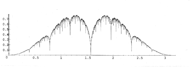
Figure 1: The function

Some properties of $f(x)$ are immediately apparent. For each factor of the infinite product, the exponent is a positive rational number with even numerator and odd denominator, so each factor is $\geq 0$ for all $x$. Because the factors are positive powers of sine functions, they are also $\leq 1$. For each $x$, the partial products are a monotonically decreasing sequence on the interval $[0,1]$, which must approach a limiting value. In other words, the partial products either converge to a number between 0 and 1, or they diverge to 0. Either way, $f(x)$ is a well-defined function with values in the range $0\leq f(x)\leq 1$ (in fact, $f(x)$ is strictly less than 1).

2 Set of zeroes

Because $\sin(2^{n}x)=0$ when $2^{n}x=m\pi$, i.e. $x=m\pi/2^{n}$, for any integer $m$, we have

(2) $$f(m\pi/2^{n})=0$$

for every integer $m$ and non-negative integer $n$. Thus the zeroes of $f$ are dense on the real line.

But $f(x)$ is not uniformly zero. For example,

(3) $$f(\pi/3)=(3/4)^{\pi^{2}/8}.$$

This follows from the fact that $2^{n}$ is congruent to 1, 2, or 4 mod 6, so that $\sin(2^{n}\pi/3)=\pm\frac{1}{2}\sqrt{3}$ and

(4) $$[\sin(2^{n}\pi/3)]^{2/(2n+1)^{2}}=(3/4)^{1/(2n+1)^{2}}.$$

Thus

(5) $$f\biggl{(}\frac{\pi}{3}\biggr{)}=\biggl{(}\frac{3}{4}\biggr{)}^{\sum_{n=0}^{\infty}1/(2n+1)^{2}}$$

($\pi^{2}/8=\pi^{2}/6-\pi^{2}/24$, the sum of the reciprocals of all squares minus the sum for even squares.)

On the other hand, $f$ has zeroes other than $x=\pi m/2^{n}$. For example, $f(x)=0$ if

(6) $$x=\pi\sum_{k=0}^{\infty}(-1)^{k}2^{-2^{2^{k}}}.$$

Indeed, if $n=2^{2^{j}}$, then

(7) $$2^{n}x=\pi\sum_{k=0}^{\infty}(-1)^{k}2^{2^{2^{j}}-2^{2^{k}}}=\pi\sum_{k=0}^{j}(-1)^{k}2^{2^{2^{j}}-2^{2^{k}}}+\pi\sum_{k=j+1}^{\infty}(-1)^{k}2^{2^{2^{j}}-2^{2^{k}}}.$$

But the sum from $k=0$ to $j$ is an integer, so

(8) $$0\leq[\sin(2^{n}x)]^{2}=\Bigl{[}\sin\Bigl{(}\pi\sum_{k=j+1}^{\infty}(-1)^{k}2^{2^{2^{j}}-2^{2^{k}}}\Bigr{)}\Bigr{]}^{2}$$

$$<\Bigl{(}\pi\sum_{k=j+1}^{\infty}(-1)^{k}2^{2^{2^{j}}-2^{2^{k}}}\Bigr{)}^{2}=\pi^{2}\Bigl{|}\sum_{k=j+1}^{\infty}(-1)^{k}2^{2^{2^{j}}-2^{2^{k}}}\Bigr{|}^{\,2}$$

$$<\pi^{2}\cdot 2^{(2^{2^{j}}-2^{2^{j+1}})2}\mbox{ (since the series is alternating)}$$

$$=\pi^{2}\cdot 2^{2(n-n^{2})}.$$

It follows that

(9) $$0\leq[\sin(2^{n}x)]^{2/(2n+1)^{2}}<\pi^{2/(2n+1)^{2}}\cdot 2^{-2(n^{2}-n)/(2n+1)^{2}}.$$

Now

(10) $$\lim_{n\to\infty}\frac{2}{(2n+1)^{2}}=0,$$

and

(11) $$\lim_{n\to\infty}\frac{-2(n^{2}-n)}{(2n+1)^{2}}=\lim_{n\to\infty}\frac{-2n^{2}+2n}{4n^{2}+4n+1}=-\frac{1}{2}\,,$$

so

(12) $$\lim_{n\to\infty}\pi^{2/(2n+1)^{2}}\cdot 2^{-2(n^{2}-n)/(2n+1)^{2}}=\pi^{0}\cdot 2^{-1/2}=\frac{1}{2}\sqrt{2}.$$

Thus, for sufficiently large $n$, the upper bound in (9) gets arbitrarily close to $\frac{1}{2}\sqrt{2}$, and in particular, beyond a certain point it becomes less than $\frac{9}{10}$, say, and stays less than $\frac{9}{10}$ for all larger $n$. A bit of experimentation reveals that this point occurs when $n=3$ (that is, $\pi^{2/49}\cdot 2^{-12/49}<\frac{9}{10}$).

Thus there are an infinite number of values of $n$ (namely $n=2^{2^{j}}$, where $j$ is any integer $\geq 1$, so that $n>3$) for which

(13) $$[\sin(2^{n}x)]^{2/(2n+1)^{2}}<\frac{9}{10}\,.$$

Since there are no values of $n$ for which

(14) $$[\sin(2^{n}x)]^{2/(2n+1)^{2}}>1,$$

it follows that

(15) $$0\leq f(x)\leq\prod_{j=1}^{\infty}\frac{9}{10}=\lim_{j\to\infty}\Bigl{(}\frac{9}{10}\Bigr{)}^{j}=0.$$

Note that $x$ is an irrational multiple of $\pi$, because the binary expansion of the sum in (6) consists of 2 zeroes, followed by 2 ones, followed by 16 zeroes, 256 ones, 65536 zeroes, etc.

Nevertheless, for “most” $x$, $f(x)>0$.

Theorem 1

The set of zeroes of $f(x)$ in the interval $0\leq x\leq\pi$ has measure $0$.

Proof: For each positive integer $k$, let

(16) $$A_{k}=\Bigl{\{}x\in[0,\pi]:\Bigl{|}x-\frac{m\pi}{2^{n}}\Bigr{|}>\frac{1}{2^{n+\sqrt{n}+k}}\mbox{ for all non-negative integers $m$ and $n$}\Bigr{\}}.$$

Some of the intervals excluded from $A_{k}$ overlap, but we can obtain a lower bound on the measure of $A_{k}$ by subtracting from $\pi$ the lengths of all the excluded intervals. When $m$ is even, $m/2^{n}$ is equal to an odd integer over a smaller power of 2, so when we add up the lengths of the excluded intervals, we can ignore even values of $m$, except for the case $m=n=0$.

Fix $n\geq 1$. There are $2^{n-1}$ odd values of $m$ for which $m\pi/2^{n}$ is in the interval $[0,\pi]$, and there is an excluded interval of length $2/2^{n+\sqrt{n}+k}$ for each such $m$. The total length of all these intervals is $1/2^{\sqrt{n}+k}$.

Summing over all $n\geq 1$, we get

(17) $$\sum_{n=1}^{\infty}\frac{1}{2^{\sqrt{n}+k}}=\frac{1}{2^{k}}\sum_{n=1}^{\infty}2^{-\sqrt{n}},$$

where

(18) $$\sum_{n=1}^{\infty}2^{-\sqrt{n}}<\int_{0}^{\infty}2^{-\sqrt{x}}\,dx.$$

With the change of variables $u=(\log 2)^{2}x$ and $z=-\sqrt{u}$, we have

(19) $$\int_{0}^{\infty}2^{-\sqrt{x}}\,dx=\int_{0}^{\infty}e^{-\sqrt{x}\log 2}\,dx=\frac{1}{(\log 2)^{2}}\int_{0}^{\infty}e^{-\sqrt{u}}\,du$$

$$=\frac{2}{(\log 2)^{2}}\int_{0}^{-\infty}ze^{z}\,dz=\frac{2}{(\log 2)^{2}}(z-1)e^{z}\biggr{|}_{\,0}^{-\infty}=\frac{2}{(\log 2)^{2}}<\frac{25}{6}\,.$$

Thus

(20) $$\sum_{n=1}^{\infty}\frac{1}{2^{\sqrt{n}+k}}<\frac{25}{6\cdot 2^{k}}\,.$$

For $n=0$, there are two excluded intervals (around 0 and $\pi$), each with length $2^{-k}$. So the total length of all excluded intervals is less than

(21) $$\frac{25}{6\cdot 2^{k}}+\frac{2}{2^{k}}=\frac{37}{6\cdot 2^{k}}\,,$$

and the measure of $A_{k}$ is greater than $\pi-37/(6\cdot 2^{k})$.

Next, we find a lower bound on $f(x)$ for $x\in A_{k}$. Suppose $0<\delta\leq\frac{1}{2}$. Then

(22) $$\sin\delta>\delta-\mbox{$\frac{1}{6}$}\,\delta^{3}=\delta(1-\mbox{$\frac{1}{6}$}\,\delta^{2})>\delta[1-\mbox{$\frac{1}{6}$}(\mbox{$\frac{1}{2}$})^{2}]=\mbox{$\frac{23}{24}$}\delta\,.$$

Now suppose $|z-\pi m|>\delta$ for every integer $m$. Then

(23) $$|\sin z|>\sin\delta>\mbox{$\frac{23}{24}$}\delta.$$

Let $n$ be any non-negative integer and suppose $|2^{n}x-\pi m|>\delta$. Then $|\sin(2^{n}x)|>\frac{23}{24}\delta$, and the same conclusion follows from the condition

(24) $$\Bigl{|}x-\frac{\pi m}{2^{n}}\Bigr{|}>\frac{\delta}{2^{n}}.$$

If $k$ is any positive integer and $n$ is any non-negative integer, then

(25) $$0<\frac{1}{2^{\sqrt{n}+k}}\leq\frac{1}{2}\,,$$

so we can let $\delta=1/2^{\sqrt{n}+k}$ and conclude that if

(26) $$\Bigl{|}x-\frac{\pi m}{2^{n}}\Bigr{|}>\frac{1}{2^{n+\sqrt{n}+k}}$$

for every integer $m$, then

(27) $$|\sin(2^{n}x)|>\frac{23}{24}\cdot\frac{1}{2^{\sqrt{n}+k}}\,.$$

In other words, if $x\in A_{k}$, so that (26) holds for every integer $m$ and every non-negative integer $n$, then (27) holds for every non-negative integer $n$. It follows that

(28) $$\log|\sin(2^{n}x)|>\log\mbox{$\frac{23}{24}$}-(\sqrt{n}+k)\log 2>-\mbox{$\frac{1}{23}$}-(\sqrt{n}+k)\log 2,$$

so

(29) $$\frac{2}{(2n+1)^{2}}\log|\sin(2^{n}x)|>\frac{-2}{23(2n+1)^{2}}-\frac{2(\sqrt{n}+k)(\log 2)}{(2n+1)^{2}}$$

$$=-\frac{\frac{2}{23}+2k\log 2}{(2n+1)^{2}}-\frac{2\sqrt{n}\log 2}{(2n+1)^{2}}.$$

Therefore

(30) $$\log f(x)=\sum_{n=0}^{\infty}\frac{2}{2n+1)^{2}}\log|\sin(2^{n}x)|$$

$$>-\sum_{n=0}^{\infty}\frac{\frac{2}{23}+2k\log 2}{(2n+1)^{2}}-(\log 2)\sum_{n=0}^{\infty}\frac{2\sqrt{n}}{(2n+1)^{2}}\,,$$

where

(31) $$\sum_{n=0}^{\infty}\frac{\frac{2}{23}+2k\log 2}{(2n+1)^{2}}=\frac{\pi^{2}}{8}\Bigl{(}\frac{2}{23}+2k\log 2\Bigr{)}$$

and

(32) $$\sum_{n=0}^{\infty}\frac{2\sqrt{n}}{(2n+1)^{2}}=\sum_{n=1}^{\infty}\frac{2\sqrt{n}}{(2n+1)^{2}}<\sum_{n=1}^{\infty}\frac{2\sqrt{n}}{(2n)^{2}}=\sum_{n=1}^{\infty}\frac{1}{2n^{3/2}}$$

$$=\frac{1}{2}+\sum_{n=2}^{\infty}\frac{1}{2n^{3/2}}<\frac{1}{2}+\int_{1}^{\infty}\frac{1}{2x^{3/2}}\,dx=\frac{1}{2}+1=\frac{3}{2}\,.$$

Thus

(33) $$\log f(x)>\frac{-\pi^{2}}{8}\Bigl{(}\frac{2}{23}+2k\log 2\Bigr{)}-\frac{3}{2}\log 2>-1.147-1.7103k$$

and

(34) $$f(x)>e^{-1.147-1.17103k}>\frac{1}{(3.15)(5.531)^{k}}\,.$$

It follows that if $f(x)\leq 1/(3.15)(5.531)^{k}$, then $x\not{\!\!\in}A_{k}$. Therefore, for every positive integer $k$, the measure of the set of all $x$ in $[0,\pi]$ for which $f(x)\leq 1/(3.15)(5.531)^{k}$ is less than $37/(6\cdot 2^{k})$, the measure of the complement of $A_{k}$. The set of $x$ for which $f(x)=0$ is a subset of the set of $x$ for which $f(x)\leq 1/(3.15)(5.531)^{k}$ for every positive integer $k$. Therefore the measure of the set of $x$ for which $f(x)=0$ is less than $37/(6\cdot 2^{k})$ for every $k$, and is thus 0.

3 Points of continuity

A function $f(x)$ is said to be upper semicontinuous [2] (p. 22) at $x=a$ if for every $\varepsilon>0$, there exists $\delta>0$ such that $f(x)<f(a)+\varepsilon$ whenever $|x-a|<\delta$. Note the asymmetry of this definition: $f(x)$ must be less than $f(a)+\varepsilon$ but need not be greater than $f(a)-\varepsilon$. Note also that continuity implies upper semicontinuity.

We shall prove that our function $f(x)$ is upper semicontinuous at all $x$. Two corollaries are that $f(x)$ is continuous at $x$ if and only if $f(x)=0$, and that $f(x)$ is Lebesgue integrable.

Theorem 2

$f(x)$ is upper semicontinuous at all $x$.

Proof: Fix $x$. We consider two cases.

Case 1: $\sin(2^{n}x)=0$ for some $n$. In this case, $2^{n}x=m\pi$ for some integer $m$, so $x=\pi m/2^{n}$. Then, because

(35) $$0\leq[\sin(2^{j}t)]^{2/(2j+1)^{2}}\leq 1$$

for all $t$ and all $j$, we have

(36) $$0\leq f(t)\leq[\sin(2^{n}t)]^{2/(2n+1)^{2}}$$

for all $t$. Since the right side of (36) is a continuous function of $t$ which is equal to 0 at $t=x$, we have $\lim_{t\to x}f(t)=f(x)$ by the squeeze theorem. Therefore $f(t)$ is continuous at $t=x$, and thus upper semicontinuous.

Case 2: $\sin(2^{n}x)$ is not equal to 0 for any non-negative integer $n$. In this case, neither is $\sin(2^{n}x)$ equal to $\pm 1$ for any $n$. For if $\sin(2^{n}x)=\pm 1$, then $2^{n}x$ is an odd multiple of $\pi/2$, in which case $2^{n+1}x$ is a multiple of $\pi$, and $\sin(2^{n+1}x)=0$. Thus

(37) $$0<[\sin(2^{n}x)]^{2/(2n+1)^{2}}<1$$

for all $n$. It follows that the partial products

(38) $$f_{k}(x)=\prod_{n=0}^{k}[\sin(2^{n}x)]^{2/(2n+1)^{2}}$$

decrease monotonically with $k$, approaching $f(x)$ as $k\to\infty$.

Given $\varepsilon>0$, we must find $\delta>0$ such that $f(t)<f(x)+\varepsilon$ whenever $|t-x|<\delta$. Let $k$ be the least non-negative integer such that $f_{k}(x)<f(x)+\varepsilon^{2}$. Note that $k$ must exist, because $f_{k}(x)$ approaches $f(x)$ monotonically from above as $k\to\infty$. Let $\lambda=f_{k}(x)$. Note that $k$ and $\lambda$ depend only on $x$ and $\varepsilon$.

If $\varepsilon\leq\frac{1}{7}$, let

(39) $$\delta=\frac{(2k+1)^{2}\lambda^{2k+1)^{2}/2}\varepsilon}{21\cdot 2^{k+1}}\,.$$

If $\varepsilon>\frac{1}{7}$, let $\delta$ have the same value that it would have for $\varepsilon=\frac{1}{7}$. Note that because $\delta$ is a function of $k$, $\lambda$, and $\varepsilon$, $\delta$ also depends only on $x$ and $\varepsilon$. We will show that if $|t-x|<\delta$, then $f(t)<f(x)+\varepsilon$.

Lemma 1

If $\varepsilon\leq\frac{1}{7}$, then $\lambda<\frac{81}{100}$.

Proof: Suppose $k=0$. Then

(40) $$f_{k}(x)-f(x)=f_{0}(x)-f(x)>f_{0}(x)-f_{1}(x)$$

$$=(\sin^{2}x)[1-(\sin 2x)^{2/9}]=(\sin^{2}x)[1-(2\sin x\cos x)^{2/9}]$$

$$\geq(\sin^{2}x)[1-(2\cos x)^{2/9}]=(\sin^{2}x)[1-(4\cos^{2}x)^{1/9}]$$

$$(\sin^{2}x)[1-4^{1/9}(1-\sin^{2}x)^{1/9}].$$

Now suppose $\sin x\geq\frac{9}{10}$. Then $\sin^{2}x\geq\frac{81}{100}$, $1-\sin^{2}x\leq\frac{19}{100}$,

(41) $$4(1-\sin^{2}x)\leq\mbox{$\frac{76}{100}$,}$$

(42) $$4^{1/9}(1-\sin^{2}x)^{1/9}\leq(\mbox{$\frac{76}{100}$})^{1/9}<\mbox{$\frac{97}{100}$,}$$

(43) $$1-4^{1/9}(1-\sin^{2}x)^{1/9}>\mbox{$\frac{3}{100}$,}$$

and

(44) $$(\sin^{2}x)[1-4^{1/9}(1-\sin^{2}x)^{1/9}]>(\mbox{$\frac{81}{100}$})(\mbox{$\frac{3}{100}$})>\mbox{$\frac{1}{49}$}\geq\varepsilon^{2}.$$

But by our definition of $k$, $f_{k}(x)-f(x)<\varepsilon^{2}$. This contradiction establishes that if $k=0$, then $\sin x<\frac{9}{10}$. Therefore

(45) $$\lambda=f_{0}(x)=\sin^{2}x<(\mbox{$\frac{9}{10}$})^{2}=\mbox{$\frac{81}{100}$.}$$

Suppose $k=1$. Then

(46) $$f_{k}(x)=f_{1}(x)=(\sin x)^{2}(\sin 2x)^{2/9},$$

which has its maximum value, just below $\frac{81}{100}$, when $\sin x=\sqrt{10/11}$. If $k>1$, then the maximum value of $f_{k}(x)$ is less than the maximum value of $f_{1}(x)$.

Lemma 2

For every non-negative integer $n$, and every real number $x$ and $t$ such that $t\neq x$, and such that $\sin(2^{n}x)$ and $\sin(2^{n}t)$ are not $0$, we have

(47) $$\log[\sin(2^{n}t)]^{2/(2n+1)^{2}}-\log[\sin(2^{n}x)]^{2/(2n+1)^{2}}<\frac{2^{n+1}|t-x|}{(2n+1)^{2}|\sin(2^{n}x)|}\,.$$

Proof: Since the righthand side of the above inequality is always positive, the inequality is satisfied whenever the lefthand side is negative. Suppose the lefthand side is positive.

Let

(48) $$g_{n}(t)=\log[\sin(2^{n}t)]^{2/(2n+1)^{2}}.$$

Then $g_{n}(t)$ is periodic with period $2^{-n}\pi$, and because $g_{n}(t)$ is an even function, we have

(49) $$g_{n}(t)=g_{n}(t+2^{-n}j\pi)=g_{n}(-t+2^{-n}j\pi)$$

for all integers $j$. Furthermore, $g_{n}(t)$ increases monotonically on each interval

(50) $$\frac{m\pi}{2^{n+1}}<t<\frac{(m+1)\pi}{2^{n+1}},$$

increasing if $m$ is even, and decreasing if $m$ is odd. Indeed, if $g_{n}(t^{\prime})=g_{n}(t)$, then $t^{\prime}$ must be equal to $t+2^{-n}j\pi$ or $-t+2^{-n}j\pi$ for some integer $j$.

Suppose $x$ and $t$ are both between $m\pi/2^{n+1}$ and $(m+1)\pi/2^{n+1}$ for some integer $m$, and suppose that $t^{\prime}$ is a real number, not between $m\pi/2^{n+1}$ and $(m+1)\pi/2^{n+1}$, such that $g_{n}(t^{\prime})=g_{n}(t)$. Then $t^{\prime}=t+2^{-n}j\pi$ or $-t+2^{-n}j\pi$ for some integer $j$. If $t^{\prime}=t+2^{-n}j\pi$, then $j\neq 0$, so $|t^{\prime}-t|\geq 2^{-n}\pi$, but $|t-x|<\pi/2^{n+1}$, so $|t^{\prime}-x|>\pi/2^{n+1}$ and $|t^{\prime}-x|>|t-x|$. If If $t^{\prime}=-t+2^{-n}j\pi$, let If $x^{\prime}=-x+2^{-n}j\pi$. Then $|t^{\prime}-x^{\prime}|=|t-x|$, and either $x<t<t^{\prime}<x^{\prime}$, $x^{\prime}<t^{\prime}<t<x$, $t<x<x^{\prime}<t^{\prime}$, or $t^{\prime}<x^{\prime}<x<t$. Whichever case applies, we have $|t^{\prime}-x|>|t-x|$. So if

(51) $$g_{n}(t)-g_{n}(x)<\frac{2^{n+1}|t-x|}{(2n+1)^{2}|\sin(2^{n}x)|},$$

then $g_{n}(t^{\prime})-g_{n}(x)$, which is equal to $g_{n}(t)-g_{n}(x)$, is less than

(52) $$\frac{2^{n+1}|t^{\prime}-x|}{(2n+1)^{2}|\sin(2^{n}x)|}.$$

Thus it suffices to prove the lemma for the case where $x$ and $t$ are both between $m\pi/2^{n+1}$ and $(m+1)\pi/2^{n+1}$ for the same integer $m$.

Now

(53) $$[\sin(2^{n}t)]^{2/(2n+1)^{2}}\geq 0$$

for all $t$, so

(54) $$g_{n}(t)=\log|\sin(2^{n}t)|^{2/(2n+1)^{2}}=\frac{2}{(2n+1)^{2}}\log|\sin(2^{n}t)|.$$

We want to find an upper bound on $|g_{n}^{\prime}(t)|$. We have

(55) $$|\sin u|=\left\{\begin{array}[]{ll}\sin u&\mbox{if }\sin u>0\\ -\sin u&\mbox{if }\sin u<0\end{array}\right\}$$

so

(56) $$\frac{d}{du}|\sin u|=\left\{\begin{array}[]{ll}\cos u&\mbox{if }\sin u>0\\ -\cos u&\mbox{if }\sin u<0\end{array}\right\}$$

and

(57) $$\frac{d}{du}\log|\sin u|=\cot u\,\mbox{ if }\sin u\neq 0.$$

Thus

(58) $$g_{n}^{\prime}(t)=\frac{2^{n+1}}{(2n+1)^{2}}\cot(2^{n}t)$$

and

(59) $$|g_{n}^{\prime}(t)|=\frac{2^{n+1}}{(2n+1)^{2}}|\cot(2^{n}t)|<\frac{2^{n+1}}{(2n+1)^{2}}\cdot\frac{1}{|\sin(2^{n}t)|}\,.$$

By hypothesis, the expression on the lefthand side of (47) is positive; that is

(60) $$\log[\sin(2^{n}t)]^{2/(2n+1)^{2}}>\log[\sin(2^{n}x)]^{2/(2n+1)^{2}}$$

so $|\sin(2^{n}t)|>|\sin(2^{n}x)|$ and

(61) $$|g_{n}^{\prime}(t)|<\frac{2^{n+1}}{(2n+1)^{2}|\sin(2^{n}x)|}\,.$$

The same upper bound holds for $|g_{n}^{\prime}(u)|$ when $u$ is between $x$ and $t$, and we also know that $g_{n}^{\prime}(u)$ has the same sign over this entire interval, because $x$ and $t$ are both between $m\pi/2^{n+1}$ and $(m+1)\pi/2^{n+1}$ for the same integer $m$. It follows that

(62) $$g_{n}(t)-g_{n}(x)=|g_{n}(t)-g_{n}(x)|=\left|\int_{x}^{t}g_{n}^{\prime}(u)\,du\right|$$

$$=\left|\int_{x}^{t}|g_{n}^{\prime}(u)|\,du\right|<\frac{2^{n+1}|t-x|}{(2n+1)^{2}|\sin(2^{n}x)|}\,.$$

This concludes the proof of Lemma 2.

  

We now continue the proof of Theorem 2. Defining $g_{n}$ as in (48), and assuming $x$ is not a multiple of $2^{-k}\pi$, so that $f_{k}(x)\neq 0$, we have

(63) $$\log f_{k}(x)=\sum_{n=0}^{k}g_{n}(x),$$

and the same holds for $t$. It follows from Lemma 2 that

(64) $$\log f_{k}(t)-\log f_{k}(x)<\sum_{n=0}^{k}\frac{2^{n+1}|t-x|}{(2n+1)^{2}|\sin(2^{n}x)|}=|t-x|\sum_{n=0}^{k}\frac{2^{n+1}}{(2n+1)^{2}|\sin(2^{n}x)|}\,.$$

From (37) we have

(65) $$\lambda=f_{k}(x)=\prod_{n=0}^{k}[\sin(2^{n}x)]^{2/(2n+1)^{2}}<[\sin(2^{n}x)]^{2/(2n+1)^{2}}=|\sin(2^{n}x)|^{2/(2n+1)^{2}}$$

for each $n$, so

(66) $$|\sin(2^{n}x)|>\lambda^{(2n+1)^{2}/2}$$

and

(67) $$\log f_{k}(t)-\log f_{k}(x)<|t-x|\sum_{n=0}^{k}\frac{2^{n+1}}{(2n+1)^{2}\lambda^{(2n+1)^{2}/2}}\,.$$

Let

(68) $$a_{n}=\frac{2^{n+1}}{(2n+1)^{2}\lambda^{(2n+1)^{2}/2}}\,.$$

Then

(69) $$\frac{a_{n+1}}{a_{n}}=\frac{2(2n+1)^{2}}{(2n+3)^{2}\lambda^{4n+4}}\,.$$

By Lemma 1, $\lambda<\frac{81}{100}$, so if $n\geq 1$, then

(70) $$\frac{a_{n+1}}{a_{n}}>\frac{2}{9}\left(\frac{81}{100}\right)^{-8}>\frac{18}{5}$$

and if $n=0$ then

(71) $$\frac{a_{n+1}}{a_{n}}>\frac{2}{9}\left(\frac{81}{100}\right)^{-4}>\frac{1}{2}\,.$$

It follows that

(72) $$\sum_{n=0}^{k}\frac{2^{n+1}}{(2n+1)^{2}\lambda^{(2n+1)^{2}/2}}<\frac{3\cdot 2^{k+1}}{(2k+1)^{2}\lambda^{(2k+1)^{2}/2}}\,,$$

and

(73) $$\log f_{k}(t)-\log f_{k}(x)<\frac{3\cdot 2^{k+1}|t-x|}{(2k+1)^{2}\lambda^{(2k+1)^{2}/2}}\,.$$

We already know that $f(t)<f_{k}(t)$, because $f_{j}(t)$ decreases monotonically with $j$, approaching $f(t)$ in the limit as $j\to\infty$. We also know that $f(t)>0$, because $f(t)>f(x)$ by hypothesis, so $\log f(t)$ is defined. Thus $\log f(t)<\log f_{k}(t)$ and

(74) $$\log f(t)<\log f_{k}(x)+\frac{3\cdot 2^{k+1}|t-x|}{(2k+1)^{2}\lambda^{(2k+1)^{2}/2}}\,.$$

We also have, by the definition of $k$, that $f_{k}(x)<f(x)+\varepsilon^{2}$. We must show that for $|t-x|$ sufficiently small, we have

(75) $$\log[f(x)+\varepsilon^{2}]+\frac{3\cdot 2^{k+1}|t-x|}{(2k+1)^{2}\lambda^{(2k+1)^{2}/2}}<\log[f(x)+\varepsilon].$$

To prove this, we consider two cases.

Case 1: $f(x)<\frac{1}{4}\varepsilon$. Then, if $f(x)\leq\frac{1}{7}$, we have $\varepsilon^{2}\leq\frac{1}{7}\varepsilon$, so $f(x)+\varepsilon^{2}<\frac{1}{4}\varepsilon+\frac{1}{7}\varepsilon<\frac{1}{2}\varepsilon$, and

(76) $$\log[f(x)+\varepsilon^{2}]<\log(\mbox{$\frac{1}{2}$}\varepsilon)=\log\varepsilon-\log 2.$$

But

(77) $$\log[f(x)+\varepsilon]\geq\log\varepsilon$$

so it suffices to have

(78) $$\frac{3\cdot 2^{k+1}\delta}{(2k+1)^{2}\lambda^{(2k+1)^{2}/2}}<\log 2,$$

or

(79) $$\delta<\frac{(\log 2)(2k+1)^{2}\lambda^{(2k+1)^{2}/2}}{3\cdot 2^{k+1}}\,.$$

Case 2: $f(x)\geq\frac{1}{4}\varepsilon$. Then

(80) $$\log[f(x)+\varepsilon^{2}]=\log\left\{f(x)\left[1+\frac{\varepsilon^{2}}{f(x)}\right]\right\}$$

$$=\log f(x)+\log\left[1+\frac{\varepsilon^{2}}{f(x)}\right]<\log f(x)+\frac{\varepsilon^{2}}{f(x)}\,.$$

Also

(81) $$\log[f(x)+\varepsilon]=\log f(x)+\log\left[1+\frac{\varepsilon}{f(x)}\right].$$

Since $\varepsilon/f(x)\leq 4$, and the $\log$ function is concave down, we have

(82) $$\log\left[1+\frac{\varepsilon}{f(x)}\right]\geq\frac{\log 5}{4}\cdot\frac{\varepsilon}{f(x)}\,.$$

Therefore

(83) $$\ \ \ \ \ \log[f(x)+\varepsilon]-\log[f(x)+\varepsilon^{2}]\geq\frac{\log 5}{4}\cdot\frac{\varepsilon}{f(x)}-\frac{\varepsilon^{2}}{f(x)}=\left[\frac{\log 5}{4}-\varepsilon\right]\frac{\varepsilon}{f(x)}\,,$$

which is

(84) $$\geq\left[\frac{\log 5}{4}-\frac{1}{7}\right]\,\frac{\varepsilon}{f(x)}>\frac{1}{7}\frac{\varepsilon}{f(x)}>\frac{1}{7}\,\varepsilon\,\mbox{ if }\,\varepsilon\leq\frac{1}{7}\,.$$

So if

(85) $$\frac{3\cdot 2^{k+1}\delta}{(2k+1)^{2}\lambda^{(2k+1)^{2}/2}}<\frac{1}{7}\varepsilon,$$

i.e. if

(86) $$\delta<\frac{(2k+1)^{2}\lambda^{(2k+1)^{2}/2}\varepsilon}{21\cdot 2^{k+1}}\,,$$

then

(87) $$\log f(t)<\log[f(x)+\varepsilon]$$

and

(88) $$f(t)<f(x)+\varepsilon.$$

If $\varepsilon\leq\frac{1}{7}$, then $\frac{1}{7}\varepsilon\leq\frac{1}{49}<\log 2$, so whether or not $f(x)<\frac{1}{4}\varepsilon$, if

(89) $$|t-x|<\frac{(2k+1)^{2}\lambda^{(2k+1)^{2}/2}\varepsilon}{21\cdot 2^{k+1}}\,,$$

then $f(t)<f(x)+\varepsilon$. This concludes the proof of Theorem 2.

  

Corollary: $f(x)$ is continuous at $x$ if and only if $f(x)=0$.

  

Proof: Because the set of zeroes of $f(x)$ is everywhere dense, $f(x)$ cannot be continuous if $f(x)\neq 0$. On the other hand, $f(x)$ is upper semicontinuous everywhere, so given $x$, for every $\varepsilon>0$, there exists $\delta>0$ such that if $|t-x|<\delta$, then $f(t)<f(x)+\varepsilon$. But $f(t)$ is never negative, so if $f(x)=0$, then $f(t)>f(x)-\varepsilon$. Therefore $f(x)$ is continuous at $x$ if $f(x)=0$.

  

Another corollary of Theorem 2 is that $f(x)$ is Lebesgue integrable, because a function that is bounded from below and upper semicontinuous on a closed interval is Lebesgue integrable over that interval [3] (p. 151). Indeed, suppose that $f(x)$ is upper semicontinuous on $[a,b]$, and let $r$ be a lower bound. Let $s$ be an upper bound of $f(x)$, which must exist, because if $\{x_{i}\}$ is a sequence of real numbers on which $f$ is unbounded, then $f$ cannot be upper semicontinuous on an accumulation point of $\{x_{i}\}$. Now suppose $f(x)<y$ for some $x\in[a,b]$ and $y\in[r,s]$. Let $\varepsilon=y-f(x)$. There exists $\delta>0$ such that $f(t)<f(x)+\varepsilon=y$ whenever $|t-x|<\delta$. In other words, if $f(x)<y$, then there is a neighborhood $U$ of $x$ such that $f(t)<y$ for all $t$ in $U$. It follows that for every $y$ in $[r,s]$, the set

(90) $$S_{y}=\{x\in[a,b]:f(x)<y\}$$

is an open set of $[a,b]$. Let $g(y)$ be the measure of $S_{y}$. Then $g(y)$ increases monotonically on the interval $[r,s]$, so $g(y)$ is Riemann integrable. But the Lebesgue integral $\int_{a}^{b}f(x)\,dx$ is equal to the Riemann integral $\int_{r}^{s}g(y)\,dy$.

4 A lower bound on the Lebesgue integral

Theorem 3

The Lebesgue integral $\int_{0}^{\pi}f(x)\,dx$ is strictly positive.

Proof: First, we prove that for all $k$, the improper integral

(91) $$\int_{0}^{\pi}\log f_{k}(x)\,dx$$

converges to a value $>-\pi^{3}/4$. We have

(92) $$\log f_{k}(x)=\sum_{n=0}^{k}\log[\sin(2^{n}x)]^{2/(2n+1)^{2}}=\sum_{n=0}^{k}\frac{2}{(2n+1)^{2}}\log|\sin(2^{n}x)|$$

(where we take both sides to be $-\infty$ when $x$ is a multiple of $2^{-k}\pi$), so

(93) $$\int_{0}^{\pi}\log f_{k}(x)\,dx=\sum_{n=0}^{k}\frac{2}{(2n+1)^{2}}\int_{0}^{\pi}\log|\sin(2^{n}x)|\,dx,$$

where the integrals on both sides are improper. By the change of variables $u=2^{n}x$, we have

(94) $$\int_{0}^{\pi}\log|\sin(2^{n}x)|\,dx=2^{-n}\int_{0}^{2^{n}\pi}\log|\sin u|\,du,$$

which, by the symmetry and periodicity of the sine function, is equal to

(95) $$2\int_{0}^{\pi/2}\log|\sin u|\,du.$$

For $0\leq u\leq\pi/2$, we have $|\sin u|=\sin u\geq 2u/\pi$, so

(96) $$\log|\sin u|\geq\log\left(\frac{2u}{\pi}\right),$$

and, by the change of variables $z=2u/\pi$, we have

(97) $$2\int_{0}^{\pi/2}\log|\sin u|\,du\geq 2\int_{0}^{\pi/2}\log\left(\frac{2u}{\pi}\right)\,du=\pi\int_{0}^{1}\log z\,dz=-\pi.$$

Therefore

(98) $$\int_{0}^{\pi}\log f_{k}(x)\,dx\geq\sum_{n=0}^{k}\frac{-2\pi}{(2n+1)^{2}}>\sum_{n=0}^{\infty}\frac{-2\pi}{(2n+1)^{2}}=-2\pi\cdot\frac{\pi^{2}}{8}=-\frac{\pi^{3}}{4}\,.$$

Now, for each positive integer $k$, let

(99) $$B_{k}=\{x\in[0,\pi]:f_{k}(x)>e^{-\pi^{2}/2}\}.$$

Because $f_{k}(x)$ is continuous, $B_{k}$ is open, and hence measurable. We want to show that the measure of $B_{k}$ is $>\pi/2$ for all $k$. The complement of $B_{k}$ in $[0,\pi]$ is

(100) $$\ \ \ \ \ \bar{B}_{k}=\{x\in[0,\pi]:f_{k}(x)\leq e^{-\pi^{2}/2}\}=\{x\in[0,\pi]:\log f_{k}(x)\leq-\pi^{2}/2\},$$

a closed set. Suppose the measure of $\bar{B}_{k}$ is $\geq\pi/2$ for some $k$. Then, because $\log f_{k}(x)\leq 0$ (incl. $-\infty$) for all $x$, and $\bar{B}_{k}$ is a subset of $[0,\pi]$, we have

(101) $$\int_{0}^{\pi}\log f_{k}(x)\,dx\leq\int_{\bar{B}_{k}}\log f_{k}(x)\,dx\leq-\frac{\pi^{2}}{2}\cdot\frac{\pi}{2}=-\frac{\pi^{3}}{4}\,,$$

but by (98), this integral is $>-\pi^{3}/4$, and this contradiction establishes that the measure of $\bar{B}_{k}$ is $<\pi/2$, and the measure of $B_{k}$ is $>\pi/2$.

Since $f_{k}(x)\geq 0$ for all $x$, we have

(102) $$\int_{0}^{\pi}f_{k}(x)\,dx\geq\int_{B_{k}}f_{k}(x)\,dx>\frac{\pi}{2}\,e^{-\pi^{2}/2}$$

for all $k$.

Now the sequence $\{f_{k}(x)\}_{k=0}^{\infty}$ converges pointwise to $f(x)$ on the interval $0\leq x\leq\pi$, and $0\leq f_{k}(x)\leq 1$ for all $x$ and all $k$. It follows from the Lebesgue dominated convergence theorem [1] (p. 183, Theorem 6.19) that

(103) $$\int_{0}^{\pi}f(x)\,dx=\lim_{k\to\infty}\int_{0}^{\pi}f_{k}(x)\,dx.$$

But $\int_{0}^{\pi}f_{k}(x)\,dx$ exists and is greater than $\frac{\pi}{2}e^{-\pi^{2}/2}$ for each $k$. It follows that $\int_{0}^{\pi}f(x)\,dx$ exists and is $\geq\frac{\pi}{2}e^{-\pi^{2}/2}$.

This concludes the proof of Theorem 3.

  

An immediate consequence of Theorem 3 is that $f(x)$ is not Riemann integrable. If it were, then the Riemann integral would be equal to the Lebesgue integral, but because the zeroes of $f(x)$ are dense on the interval $[0,\pi]$, every lower Riemann sum is zero.

However, we do have

Theorem 4

The lim inf of the upper Riemann sums of $f(x)$ is equal to the Lebesgue integral.

Proof: Let $R$ be the set of partitions of the interval $[0,\pi]$ into a finite number of intervals, and let $L$ be the set of partitions of $[0,\pi]$ into a finite number of Borel sets. Let

(104) $$U_{R}=\liminf_{{\cal P}\in R}\sum_{S\in{\cal P}}\mu(S)\limsup_{x\in S}f(x)$$

and let

(105) $$U_{L}=\liminf_{{\cal P}\in L}\sum_{S\in{\cal P}}\mu(S)\limsup_{x\in S}f(x)$$

where $\mu$ is Borel measure. Because every interval is a Borel set, $R$ is a subset of $L$, and $U_{R}\geq U_{L}$.

For each $k$, let

(106) $$U_{R,k}=\liminf_{{\cal P}\in R}\sum_{S\in{\cal P}}\mu(S)\limsup_{x\in S}f_{k}(x).$$

For each $k$, $f(x)\leq f_{k}(x)$ for all $x$, so $U_{R}\leq U_{R,k}$. Also, for each $k$, $f_{k}(x)$ is continuous, and hence Riemann integrable. By the Lebesgue dominated convergence theorem [1] (p. 183), the Riemann integral of $f(x)$, and hence $U_{L}$, is equal to the limit as $k\to\infty$ of the Lebesgue integral of $f_{k}(x)$ (and hence the Riemann integral of $f_{k}(x)$, and $U_{R,k}$). Therefore $U_{R}\leq U_{L}$. Since $U_{R}$ is both $\geq$ and $\leq U_{L}$, $U_{R}=U_{L}$, and since $f(x)$ is Lebesgue integrable, $U_{R}$ is equal to the Lebesgue integral.

5 A numerical estimate

How can we find a decimal value for $\int_{0}^{\pi}f(x)\,dx$? The usual numerical integration methods, such as Simpson’s rule, are unstable for this function. However, $\int_{0}^{\pi}f_{k}(x)\,dx$ converges to $\int_{0}^{\pi}f(x)\,dx$ as $k\to\infty$, and $f_{k}(x)$ is continuous, so we can estimate $\int_{0}^{\pi}f(x)\,dx$ by estimating $\int_{0}^{\pi}f_{k}(x)\,dx$.

Let $M_{k}$ be the midpoint estimate of $2\int_{0}^{\pi/2}f_{k+1}(x)\,dx$ (which is equal to $\int_{0}^{\pi}f_{k+1}(x)\,dx$) with $2^{k}$ intervals. Then

(107) $$M_{k}=\frac{\pi}{2^{k}}\sum_{j=1}^{2^{k}}\bigl{[}\sin\bigl{(}(2j-1)2^{n-k-2}\pi\bigr{)}\bigr{]}^{2/(2n+1)^{2}}.$$

(In the above equation, we need only compute the product up to $n=k$, instead of $n=k+1$, because the sine of any odd multiple of $\frac{\pi}{2}$ is $1$.) Let

(108) $$M_{\infty}=\lim_{k\to\infty}M_{k}.$$

We conjecture that $M_{\infty}$ exists and is equal to $\int_{0}^{\pi}f(x)\,dx$. This does not, of course, follow from the fact that for fixed $k$, the midpoint estimate of $\int_{0}^{\pi}f_{k+1}(x)\,dx$ with $2^{m}$ intervals converges to this integral as $m\to\infty$, and $\int_{0}^{\pi}f_{k+1}(x)\,dx$ converges to $\int_{0}^{\pi}f(x)\,dx$ as $k\to\infty$.

Table 1 shows the values of $M_{k}$ for $6\leq k\leq 29$, in column 2. Column 3 shows the reciprocal square roots of the differences $M_{k-1}-M_{k}$. The fact that these grow linearly with $k$ means that the differences decrease as $1/k^{2}$, which is what we would expect, given that $\int_{0}^{\pi}[\sin(2^{n}x)]^{2/(2n+2)^{2}}\,dx=\pi-O(1/n^{2})$. This in turn suggests that the errors $M_{k}-M_{\infty}$ decrease as $1/k$. We might expect that for a suitable choice of constants $a$ and $b$, $M_{k}-a(k-b)^{-1}$ should converge to $M_{\infty}$ much more rapidly than $M_{k}$ itself. A bit of trial and error reveals that the values $a=.4044$ and $b=.27$ work nicely. Column 4 shows the values of $M_{k}-.4044(k-.27)^{-1}$. To 5 decimal places, $\int_{0}^{\pi}f(x)\,dx$ appears to be $1.16993\dots$

$k$	$M_{k}$	$(M_{k-1}-M_{k})^{-1/2}$	$M_{k}-.4044/(k-.27)$
6	1.2419727451		1.1713968
7	1.2311527243	9.613598	1.1710636
8	1.2230892609	11.136255	1.1707736
9	1.2168748353	12.685264	1.1705518
10	1.2119511226	14.251272	1.1703889
11	1.2079596568	15.828283	1.1702709
12	1.2046613111	17.412130	1.1701856
13	1.2018911808	18.999838	1.1701237
14	1.1995322446	20.589315	1.1700785
15	1.1974993737	22.179160	1.1700452
16	1.1957292786	23.768496	1.1700204
17	1.1941739924	25.356823	1.1700019
18	1.1927965318	26.943897	1.1699877
19	1.1915679404	28.529638	1.1699769
20	1.1904652307	30.114067	1.1699685
21	1.1894699246	31.697256	1.1699620
22	1.1885669999	33.279304	1.1699568
23	1.1877441184	34.860317	1.1699527
24	1.1869910513	36.440403	1.1699493
25	1.1862992466	38.019661	1.1699466
26	1.1856614980	39.598181	1.1699444
27	1.1850716898	41.176044	1.1699426
28	1.1845245979	42.753322	1.1699411
29	1.1840157324	44.330078	1.1699399

Table 1:

I would like to thank Daniel Asimov for his assistance computing the numbers in Table 1.

References

[1] David M. Bressoud, A Radical Approach to Lebesgue’s Theory of Integration, Cambridge U. Press, 2008.
[2] Bernard R. Gelbaum and John M. H. Olmsted, Counterexamples in Analysis, Holden Day, 1964.
[3] Thomas Hawkins, Lebesgue’s Theory of Integration: Its Origins and Development, Am. Math. Soc., 2001.