Fast optimization of
Multithreshold Entropy Linear Classifier
e-mail: rafjoz@gmail.com
2Faculty of Mathematics and Computer Science
Jagiellonian University
ul. Lojasiewicza 6, 30-389 Krakow
e-mail: w.czarnecki@uj.edu.pl )
Abstract
Multithreshold Entropy Linear Classifier (MELC) is a density based model which searches for a linear projection maximizing the Cauchy-Schwarz Divergence of dataset kernel density estimation. Despite its good empirical results, one of its drawbacks is the optimization speed. In this paper we analyze how one can speed it up through solving an approximate problem. We analyze two methods, both similar to the approximate solutions of the Kernel Density Estimation querying and provide adaptive schemes for selecting a crucial parameters based on user-specified acceptable error. Furthermore we show how one can exploit well known conjugate gradients and L-BFGS optimizers despite the fact that the original optimization problem should be solved on the sphere. All above methods and modifications are tested on 10 real life datasets from UCI repository to confirm their practical usability.
1 Introduction
Many methods of speeding up the kernel density estimator’s (KDE) querying process has been proposed in the literature [12, 14, 6]. As optimization problem introduced in Multithreshold Entropy Linear Classifier [5] is closely related to the equations of KDE it appears natural that similar techniques can be used to simplify its computations with a bounded error. Importance of such reductions comes from the high (quadratic) complexity of the evaluation of functions required during training of this model which makes it hard to use for any dataset with more than a thousand points. In this paper we investigate two such approaches, first – sorting and discarding, which ignores computations of similarities between points that are too far away to have big impact on the function’s value, second – binning, which smooths the function construction in order to heavily reduce amount of unique points. Both these methods are introduced in an adaptive manner so the optimization process have fixed error bound despite many different linear projections being analyzed during the training phase. We also show a very simple method which enables to use a wide range of optimization algorithms even though proposed model requires optimization with a specific constraints (sphere bounded).
2 Multithreshold Entropy Linear Classifier
Multithreshold Entropy Linear Classifier (MELC [5]) has been recently proposed as an information theoretic approach for building model from the multithreshold linear family [1]. It’s core idea is to find a linear operator (with unit norm) such that kernel density estimations of projected classes’ training samples maximize the Cauchy-Schwarz Divergence (D [9]). Let us recall the equation of D in order to find the core computational bottleneck which appears in MELC optimization
for being a kernel density estimator of with Silverman’s rule [11], thus from the definition of Renyi’s quadratic entropy, Renyi’s quadratic cross entropy and the fact that we have
As whole D function is composed of evaluations, in the rest of our paper we focus purely on the , which we expand using Gaussian kernel density estimation [5] and denote .
where is a sum of each classes estimated variances using Silverman’s rule [11].
In an obvious way, naive computation of is , where due to the summation over all possible pairs . In the following sections we focus on methods which reduce this computational bottleneck while still preserving given approximation of value.
3 Reduction of computational complexity
Sorting and discarding
Let us begin with the very simple conception of computing values of only those pairs which are close enough to have an impact on the value of . If we assume that points projections are sorted (which can be done in general in 111in fact for iterative optimization techniques points ordering does not change much between subsequent calls so after initial sorting it can be done in linear time using insertion sort) we can search the dataset in linear time and identify for each point indices of first and last point which are at most at distance from . Following theorem shows what to choose in order to obtain at most error.
Theorem 1.
Using adaptive sorting and discarding with distance threshold in each iteration of at least
where is a sum of each classes estimated variances, leads to the computation of the function with at most error, assuming that at most fraction of points is located closer than .
Proof.
We assume that for pairs of points which are being ignored during computation of so thus
If we look for an approximation of non-regularized MELC objective we put and consequently
thus
obviously if then any satisfies this inequality (as it can only happen if we choose very big acceptable error ), so for simplicity we add the maximum of this value with .
∎
Binning
While sorting and discarding technique is quite easy to implement and analyze its practical speedup might be limited for densely packed datasets. In such cases it might be more valuable to perform a binning of our projected points, so those located near each other are approximated by their empirical mean. Such an approach works well for densely packed datasets which makes it a complementary approach to the previous one.
Let us assume that we have some partitioning of the where each is an interval. We define a binning operator as , where . We use following notation for simplicity .Similarly to the previous strategy, in order to preserve good approximation, bins width () needs to be adapted in each iteration and the exact equation is given in the following theorem.
Theorem 2.
Using adaptive binning technique with bin width in each iteration at most
where is a sum of each classes estimated variances, leads to the computation of the function with at most error.
Proof.
we assume that so
Let us now assume that we are given some acceptable error . We will show how small bins have to be used based on our dataset and current projection.
but , so
thus
Naturally if then any satisfies this inequality (similarly to the sorting and discarding method, it may only happen if we choose very large acceptable error ) so we introduce maximum function here.
∎
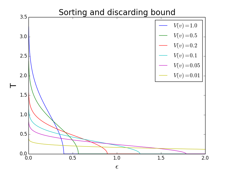
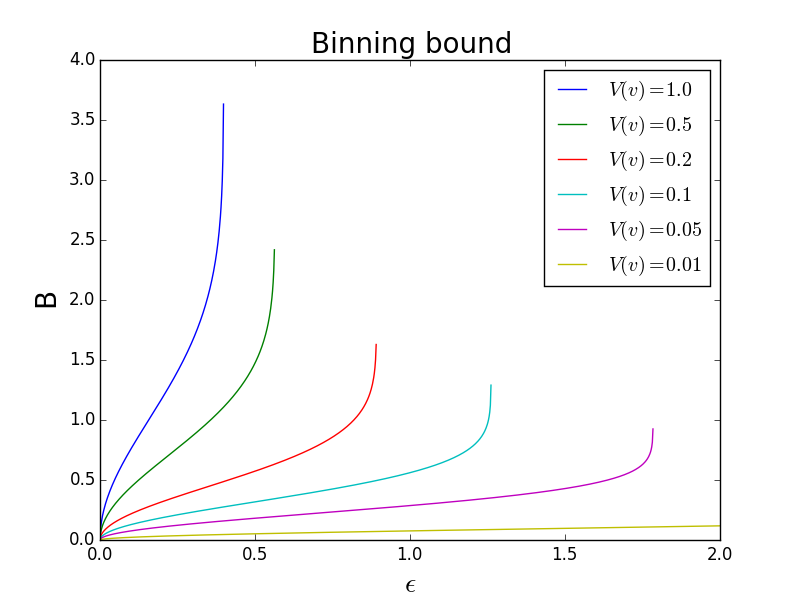
Figure 1 shows how these two bounds behave with increasing size of the acceptable error. In particular one can see that both methods have very similar growth (up to the maximization/minimization symmetry) with changing . As a result, due to the fact that binning is much more aggressive technique we should expect that using these bounds as the actual bin width/discarding threshold will lead to much greater reduction of the computational complexity when using binning.
4 Out of sphere optimization
Now we are going to show, that MELC objective function can be efficiently optimized in the whole space by adding some custom regularization term. The importance of this result is the fact that it enables us to use vast amount of existing optimization techniques (such as Adaptive gradient descent, Conjugate Gradients, BFGS, L-BFGS etc.) without adapting them to the sphere constraints. The second important aspect is the fact that this modification does not involve adding any additional constants which have to be fitted. Following theorem describes modified objective function.
Theorem 3.
Given arbitrary sets and corresponding function we have:
and
Proof.
According to [5], D is scale invariant so for any
As a result also
but as and we have that is maximized for with norm and that it is equal to . As a result sets of solutions of both problems are identical.
∎
Consequently we can apply any advanced optimization technique which is not designed to work on the sphere to optimize D criterion. In particular we can use L-BFGS [3] instead of more complex and less popular RBFGS [10] and previously proposed [5] less efficient – gradient descent on sphere method. At the same time the norm of the candidate solution will stay close to so we will not suffer from numerical problems [5].
It is worth noting that despite similarity to the L2 regularization [13] of the additive loss function (or weight decay from neural networks) this additional terms serves no regularization purposes nor it affects the actual function value. It only guides the gradient based optimizers towards more informative regions of the state space.
From the practical point of view we also need a gradient of the new function but thanks to the additivity of derivative operator we get
and we can use any optimization software able to maximize a function given (.
5 Evaluation
We evaluate proposed approximations on 10 datasets from UCI repository [2] and libSVM’s repository [4, 7]. Both D and approximations are coded in Python using numpy and scipy [8]. We use scipy’s optimization module to perform training of all models using two optimization techniques – Conjugate Gradients (CG) and L-BFGS-B [3]. Each experiment is performed in cross validation manner with multiple starting points (randomly selected, but constant across methods to achieve comparable results) due to the convergence of MELC optimization to local optima. We analyze hyperparameter of D in and acceptable error . Similarly to the original paper we use Balanced Accuracy (BAC222) as the measure of classification correctness due to MELC highly balanced formulation.
First, we investigate how big is mean reduction of computations using each of the approximating schemes. Table 1 reports mean ratio of exp function calls (which is equivalent to number of pairs analyzed in each evaluation when optimizing whole D function and its gradient) in given method to the original implementation.
| method | CG | L-BFGS-B | ||
|---|---|---|---|---|
| name | bin | dist | bin | dist |
| australian | 0.11 | 0.44 | 0.11 | 0.45 |
| breast-cancer | 0.10 | 0.46 | 0.10 | 0.46 |
| diabetes | 0.21 | 0.56 | 0.22 | 0.54 |
| fourclass | 0.19 | 0.51 | 0.19 | 0.49 |
| german.numer | 0.15 | 0.47 | 0.19 | 0.46 |
| heart | 0.29 | 0.47 | 0.26 | 0.47 |
| ionosphere | 0.25 | 0.55 | 0.24 | 0.54 |
| liver-disorders | 0.29 | 0.65 | 0.31 | 0.67 |
| sonar | 0.32 | 0.53 | 0.29 | 0.50 |
| splice | 0.19 | 0.44 | 0.16 | 0.43 |
One can easily notice that sorting and discarding method (denoted as ”dist”) roughly halves the number of analyzed pairs, while binning (denoted as ”bin”) reduces it 3-10 times. It is an obvious consequence of the fact that binning is much more aggressive method. It appears that strength of reduction depends only on the dataset, not on the optimization algorithm used which suggests, that projections for which particular level of possible reduction are uniformly distributed over the space of all projections. These effects are also heavily dependent333we do not include the exact values in the Table for better readability on the choice of and which is the obvious consequence of Theorems 1 and 2 saying that with increasing variance (which is proportional to ) the reduction strength decreases superlinearly.
The set of heat maps in Figure 2 shows differences between BAC obtained by the original D and each approximation for a given dataset and hyperparameters pair. In general, up to few isolated cases errors are on the level of . For small values errors introduced by the approximation are significantly higher and for sonar and splice datasets can grow to even . Fortunately, these are very rare phenomena.
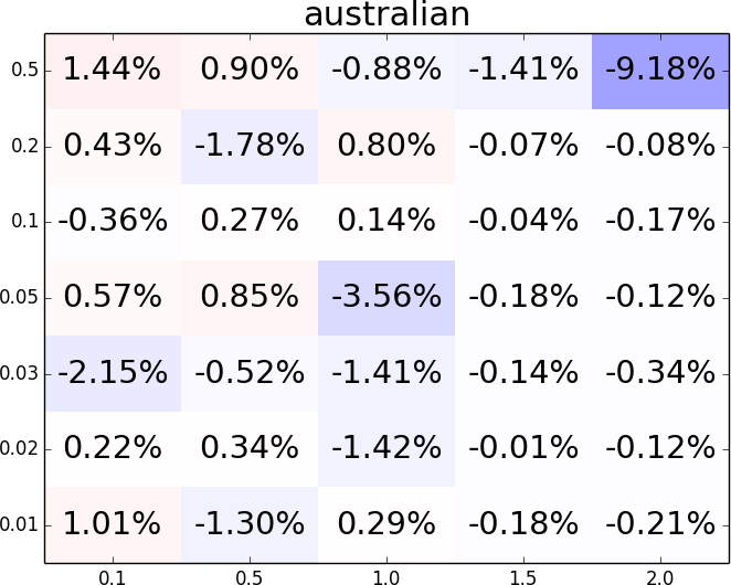
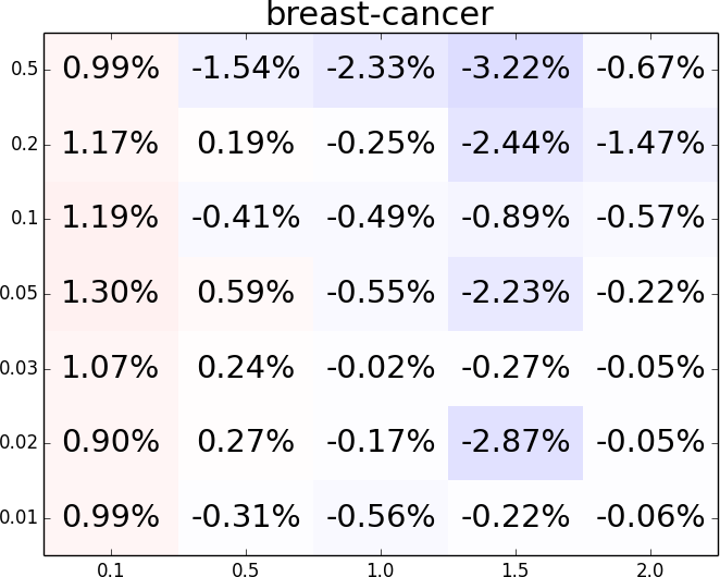
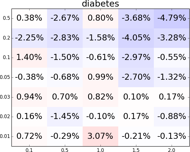
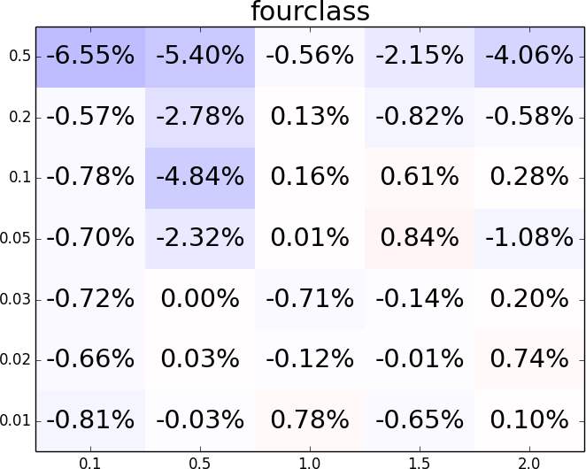
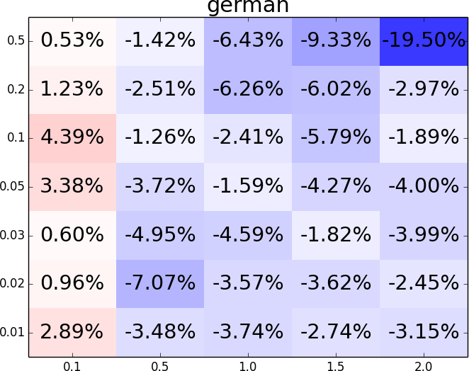
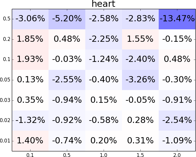
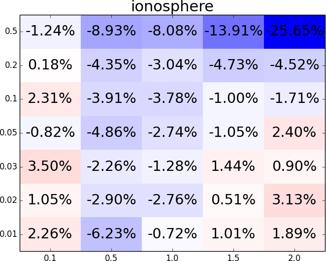
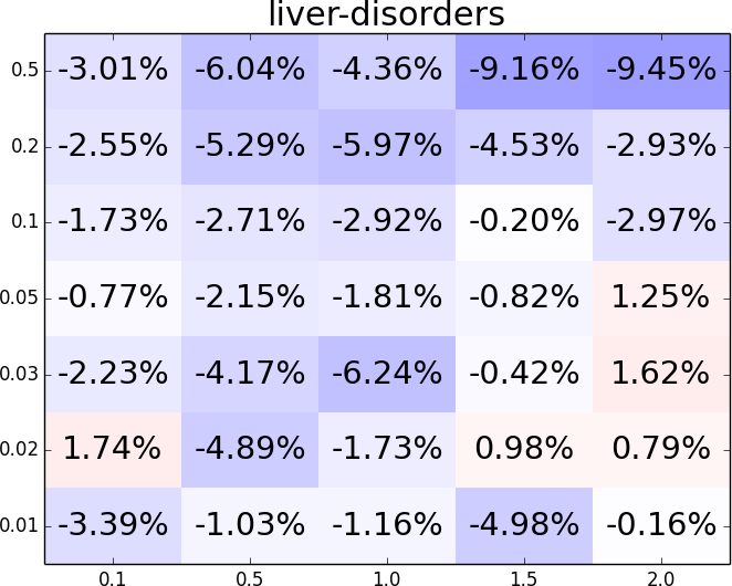
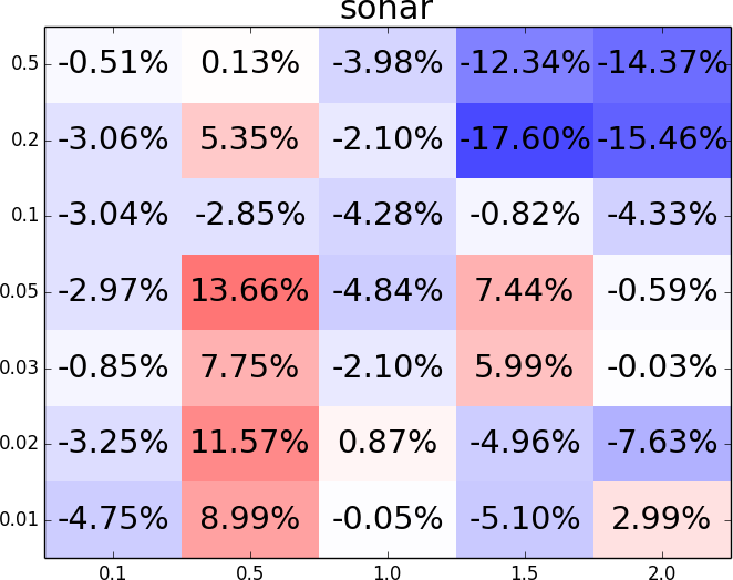
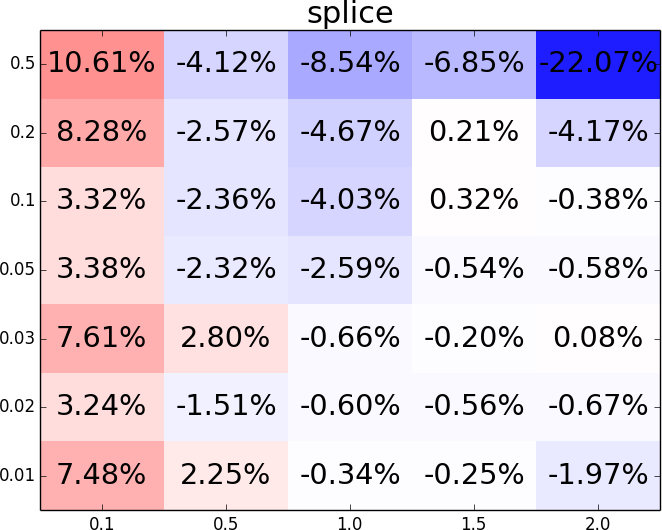
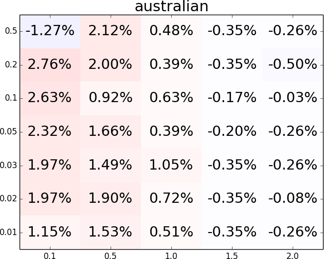
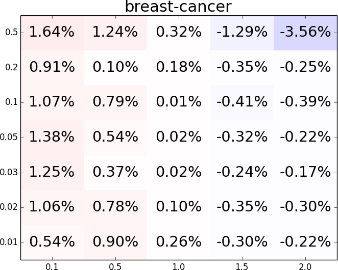
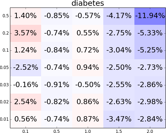
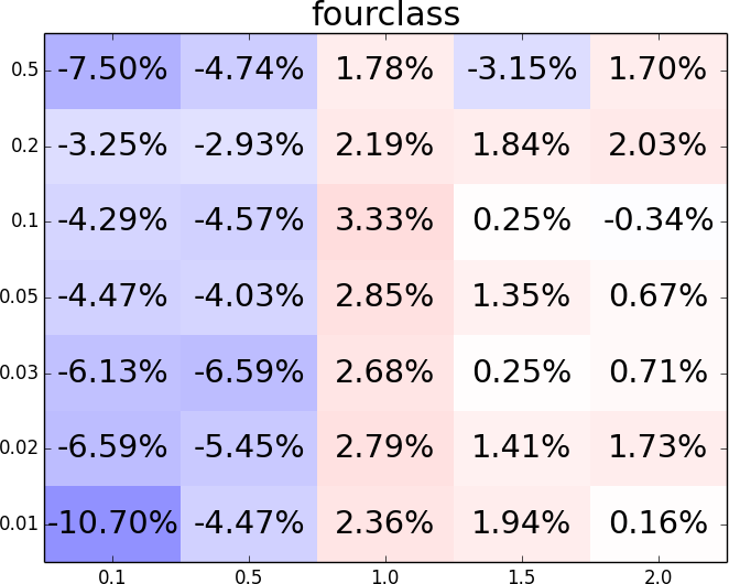
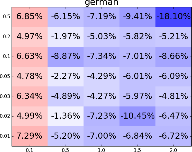
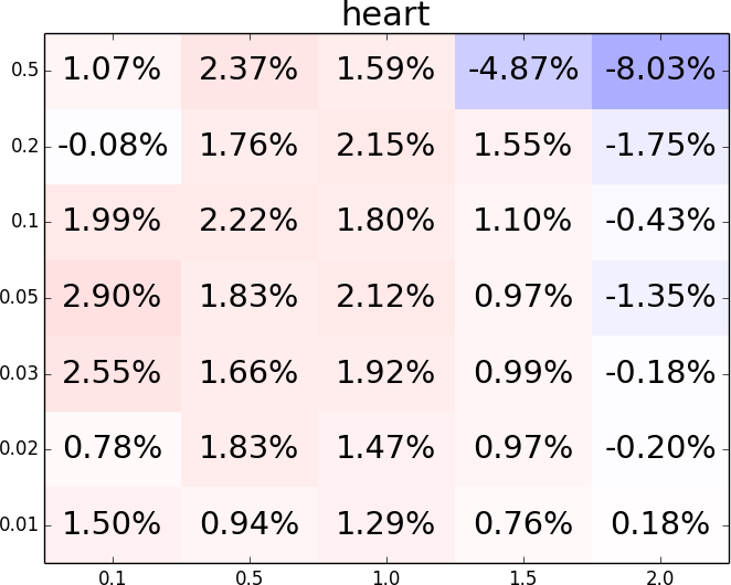
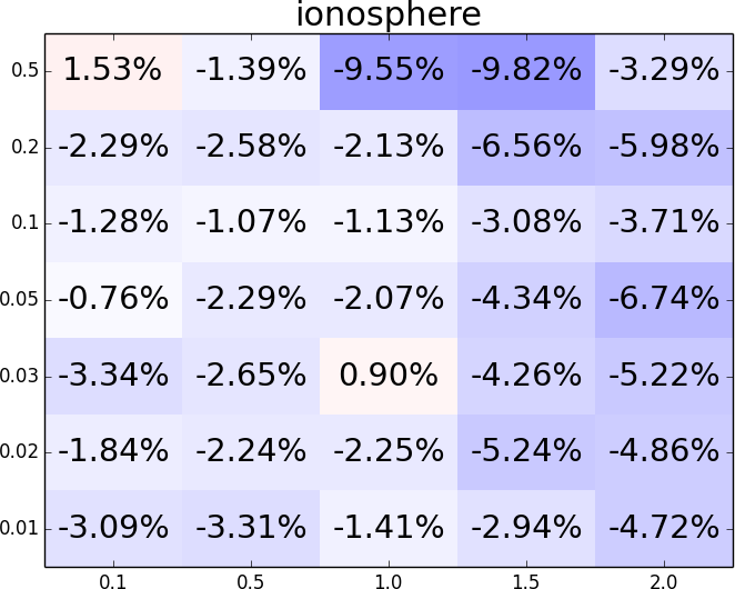
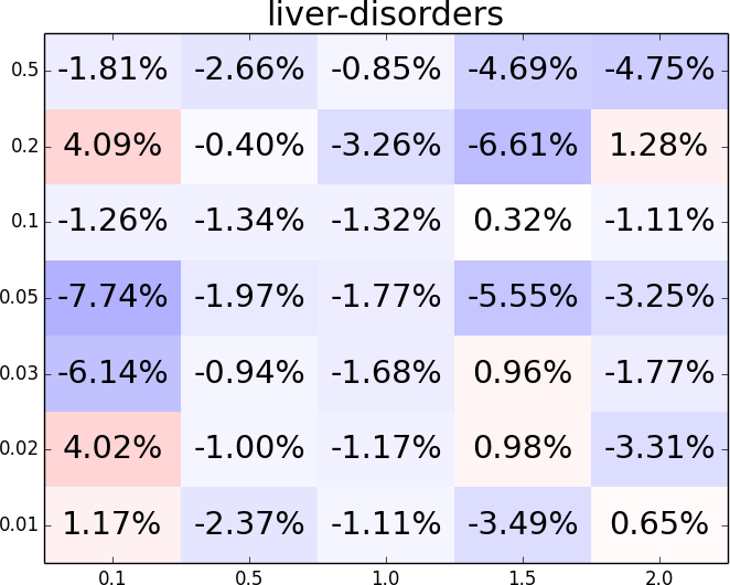
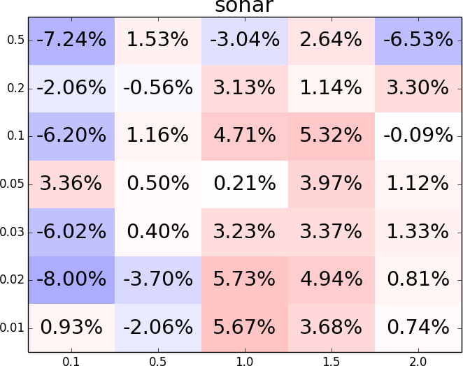
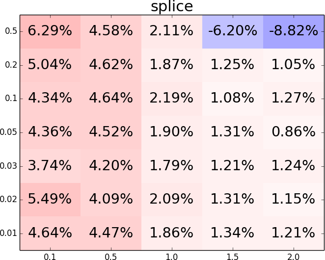
Even more interesting is the fact that for many experiments we actually noticed increase in the BAC score (bluish elements). This might be the consequence of more rough evaluation of the function (and gradient) values leading to optimization less prone to falling into local maxima. Our hypothesis is that it acts like a regularization helping to train MELC model.
Analysis of the number of iterations of each optimization method required to converge (see Table 2) shows that both approximations significantly simplify the problem. It is important to notice that the number of iterations is not the number of D function evaluations (as both Conjugate Gradients and L-BFGS-B evaluate it multiple times in each iteration, especially during line searches). Consequently, number of iterations cannot be used as a measure of optimization speed but it says much about the complexity of the function being maximized.
| method | CG | L-BFGS-B | |||||
|---|---|---|---|---|---|---|---|
| name | bin | D | dist | bin | D | dist | |
| australian | 4 | 36 | 22 | 11 | 39 | 37 | |
| breast-cancer | 4 | 35 | 8 | 6 | 39 | 14 | |
| diabetes | 3 | 30 | 20 | 18 | 36 | 29 | |
| fourclass | 4 | 12 | 10 | 6 | 15 | 14 | |
| german.numer | 7 | 60 | 32 | 7 | 58 | 38 | |
| heart | 3 | 40 | 19 | 12 | 34 | 20 | |
| ionosphere | 5 | 600 | 216 | 18 | 384 | 152 | |
| liver-disorders | 4 | 30 | 22 | 22 | 43 | 30 | |
| sonar | 4 | 262 | 115 | 15 | 139 | 100 | |
| splice | 4 | 92 | 26 | 14 | 65 | 41 | |
This seems to confirm our claim that approximation works similar to the regularization and thus it reduces small irregularities of the error surface due to the removal of small elements from the internal summation.
Experiments also showed importance on the regularization technique added to perform out of sphere optimization. During maximization of D in sonar and german datasets, norms of rapidly grew to over if we turn off this modification and still use CG/L-BFGS-B. As a result the optimization problem became extremely hard and we needed tens of thousands D evaluation in order to converge. Adding regularizing term reduced the norm to nearly and number of required function calls by two orders of magnitude.
6 Conclusions
In this paper we proposed two simple approximation schemes for faster computation of MELC objective function and its gradient. We proved that in order to achieve constant error bound during optimization one needs a specific adaptive strategy for each of them and gave a simple, closed form equations for setting required parameters based on the user-specified acceptable level of error in the function value. We also showed how one can easily change the objective function in order to use wide range of existing optimizers while at the same time still work near the unit sphere which, as described in the MELC theory [5], is important from the numerical point of view.
During extensive evaluation we confirmed that such approach is valid in terms of reducing the mean number of calls by even an order of magnitude while not sacrificing the resulting classifiers accuracy. In fact the experiments suggest that proposed method acts like some kind of regularization which might not only simplify the optimization problem but also slightly increase the obtained results.
References
- [1] Martin Anthony. Partitioning points by parallel planes. Discrete mathematics, 282(1):17–21, 2004.
- [2] Catherine Blake and Christopher J Merz. UCI repository of machine learning databases. 1998.
- [3] Richard H Byrd, Peihuang Lu, Jorge Nocedal, and Ciyou Zhu. A limited memory algorithm for bound constrained optimization. SIAM Journal on Scientific Computing, 16(5):1190–1208, 1995.
- [4] Chih-Chung Chang and Chih-Jen Lin. Libsvm: a library for support vector machines. ACM Transactions on Intelligent Systems and Technology (TIST), 2(3):27, 2011.
- [5] Wojciech Marian Czarnecki and Jacek Tabor. Multithreshold entropy linear classifier: Theory and applications. Expert Systems with Applications, 2015.
- [6] Ahmed Elgammal, Ramani Duraiswami, and Larry S Davis. Efficient kernel density estimation using the fast gauss transform with applications to color modeling and tracking. IEEE Transactions on Pattern Analysis and Machine Intelligence, 25(11):1499–1504, 2003.
- [7] Tin Kam Ho and Eugene M Kleinberg. Building projectable classifiers of arbitrary complexity. In Pattern Recognition, 1996., Proceedings of the 13th International Conference on, volume 2, pages 880–885. IEEE, 1996.
- [8] Eric Jones, Travis Oliphant, and Pearu Peterson. Scipy: Open source scientific tools for python. http://www. scipy. org/, 2001.
- [9] Jose C Principe. Information theoretic learning: Rényi’s entropy and kernel perspectives. Springer, 2010.
- [10] Chunhong Qi, Kyle A Gallivan, and P-A Absil. Riemannian bfgs algorithm with applications. In Recent advances in optimization and its applications in engineering, pages 183–192. Springer, 2010.
- [11] Bernard W Silverman. Density estimation for statistics and data analysis, volume 26. CRC press, 1986.
- [12] BW Silverman. Algorithm as 176: Kernel density estimation using the fast fourier transform. Applied Statistics, pages 93–99, 1982.
- [13] Vladimir Vapnik. The nature of statistical learning theory. springer, 2000.
- [14] Changjiang Yang, Ramani Duraiswami, Nail A Gumerov, and Larry Davis. Improved fast gauss transform and efficient kernel density estimation. In Proceedings of the Ninth IEEE International Conference on Computer Vision, pages 664–671. IEEE, 2003.