A Pseudospectral Method for Gravitational Wave Collapse
Abstract
We present a new pseudospectral code, bamps, for numerical relativity written with the evolution of collapsing gravitational waves in mind. We employ the first order generalized harmonic gauge formulation. The relevant theory is reviewed and the numerical method is critically examined and specialized for the task at hand. In particular we investigate formulation parameters, gauge and constraint preserving boundary conditions well-suited to non-vanishing gauge source functions. Different types of axisymmetric twist-free moment of time symmetry gravitational wave initial data are discussed. A treatment of the axisymmetric apparent horizon condition is presented with careful attention to regularity on axis. Our apparent horizon finder is then evaluated in a number of test cases. Moving on to evolutions, we investigate modifications to the generalized harmonic gauge constraint damping scheme to improve conservation in the strong field regime. We demonstrate strong-scaling of our pseudospectral penalty code. We employ the Cartoon method to efficiently evolve axisymmetric data in our dimensional code. We perform test evolutions of Schwarzschild perturbed by gravitational waves and by gauge pulses, both to demonstrate the use of our blackhole excision scheme and for comparison with earlier results. Finally numerical evolutions of supercritical Brill waves are presented to demonstrate durability of the excision scheme for the dynamical formation of a blackhole.
pacs:
95.30.Sf, 04.25.D-I Introduction
This is the first in a series of papers about the numerical treatment of collapsing gravitational waves using a new pseudospectral code developed for the problem. In the early s critical phenomena were discovered in gravitational collapse Cho91 , in spherical symmetry, with general relativity minimally coupled to a massless scalar field. One aspect of the finding was that, amazingly, the critical solution dividing the formation of a blackhole from dissipation of the field, was unique, in the sense that if one takes any one parameter family of initial data, with the parameter controlling somehow the strength of the data, and tunes this parameter to the threshold of blackhole formation, one finds that the same solution is always obtained, regardless of the family! Shortly thereafter similar phenomenology was reported in axisymmetric, vacuum general relativity AbrEva92 , or in other words in the collapse of gravitational waves. Since then multiple studies have been performed to reproduce this finding, albeit with different initial data and numerical approaches, but without success. Perhaps most strikingly, in Sor10 , numerical evidence of a different critical solution was presented. Even if one completely accepts the available evidence for criticality in vacuum collapse, this obviously begs the question whether or not the naive expectation of uniqueness of the critical solution in axisymmetric, rather than spherical, collapse holds.
Roughly speaking there are two types of code being used used in 3d numerical relativity. The first uses the moving puncture method BakCenCho05 ; CamLouMar05 , which consists, in essence, of a clever choice of evolved variables and gauge conditions, normally treated numerically by finite differencing. Secondly is the pseudospectral method, most prevalently used with a first order generalized harmonic formulation of general relativity by the SpEC code SpEC . Recently, we presented a study of the collapse of gravitational waves using the moving puncture method HilBauWey13 , in part to establish how close to the critical regime one can get with this standard approach. The conclusion being; not very. Major difficulties included the formation of coordinate singularities and a lack of accuracy. Therefore one would like to tackle the problem using the pseudospectral approach to establish what can be achieved in that setting. We have thus developed a new pseudospectral code along the lines of SpEC, specializing the continuum and numerical method as much as possible towards the problem of vacuum gravitational collapse. The present paper represents the first outcome of this maneuver. Herein we describe the formulation of GR employed, our boundary conditions, the code, calibration of the method, our initial data, our approach to axisymmetric apparent horizons, plus a suite of validation tests for gauge waves, gravitational waves, blackhole and collapse spacetimes. Throughout we compare our results carefully with those in the literature. We aim to give a body of evidence for the correctness of the method that the reader will find compelling. With this out of the way, in subsequent papers we turn to the problem of critical collapse. A summary follows before the main text.
In section II we look at a slightly modified version of the first order generalized harmonic formulation of LinSchKid05 . We consider constraint preserving, radiation controlling boundary conditions, paying special attention to the constraint preserving boundaries. By considering the reflection of outgoing waves in the linear approximation we ultimately suggest modified conditions that should reduce spurious reflections caused by the use of constraint damping. We also suggest alternative gauge boundary conditions.
Next, in section III, we outline the bamps code, including our carefully constructed cubed-sphere grids, which avoid clustering of grid-points in unfortunate positions of the domain. For the discretization we employ a pure Chebyschev approach. We also discuss our ‘octant’ symmetry implementation, the crucial patching-penalty approach for communicating data between neighboring coordinate patches, and finally the boundary implementation. In the follow-up section IV we complete the presentation of the penalty method by computing the penalty parameters appropriate for the semi-discrete system.
Given the difficulties in the literature in reproducing the results of AbrEva92 it seems necessary to solve the problem in axisymmetry before moving to examine the collapse of fully 3d waves without symmetry. In our moving puncture gauge study HilBauWey13 a major disadvantage in using the BAM code was that 3d grids were employed to evolve axisymmetric data. In section V we present our approach to evolving axisymmetric spacetimes with the bamps code, for which we employ the Cartoon method AlcBraBru99a to reduce from the standard bamps 3d domains to a plane, by using the Killing vector to evaluate any angular derivatives. We discuss various flavors of axisymmetric moment-of-time-symmetry initial data and their numerical construction. These initial data sets are evolved in a forthcoming study. We also give a detailed description of our formulation of the apparent horizon conditions in axisymmetry. To the best of our knowledge this is the first time that the regularity conditions on the symmetry axis have been carefully taken care of. This is important in later work as the search for apparent horizons will be our key diagnostic tool.
The next three sections (VI-VIII) contain a write-up of our development and validation tests. The tests include evolutions with the proposed gauge boundary conditions, which we find are helpful when using large gauge source parameters, as desired. They also include runs comparing the fully 3d, octant symmetry and Cartoon evolutions, demonstrating that the various symmetry setups are well-behaved. In the evolution of single blackholes we test different gauges and boundary conditions, and following LinSchKid05 , look at evolutions in which the blackhole is perturbed by a gravitational wave injected through the outer boundary. Our results are in good agreement with the earlier studies. We then examine the evolution of supercritical Brill waves, where, after the formation of an apparent horizon the run is continued after interpolation onto an excision grid, as used to evolve a single blackhole, which is needed to evolve data with a horizon for long-times. Finally we conclude in section IX.
II The generalized harmonic formulation and boundary conditions
II.1 GHG, constraints, boundary conditions
The evolution system:
We use the first order reduction of the generalized harmonic formulation with several free parameters. The full reduction from the second order Einstein equations is presented in detail elsewhere LinSchKid05 so here we give only a brief overview to establish our notation. Throughout the paper in continuum equations we use the latin for four dimensional indices, but for spatial indices, with the exception of and , whose meaning when used as indices will be described shortly. Greek indices are used to refer to the position in a state-vector, grid indices, or where otherwise needed. We start from the vacuum generalized harmonic formulation in second order form,
| (1) |
for the unknown spacetime metric with Christoffels . The constraints of the system are , plus the standard Hamiltonian and momentum constraints of GR. The gauge source functions are freely specifiable, provided that they do not include derivatives of the metric, which would affect the principal part of the PDE. The terms involving are included so as to damp away high-frequency constraint violations GunGarCal05 . The parameters and control whether or not the constraint addition made in the construction of the formulation is done either with the covariant or the partial derivative, or some combination. The latter choice has the effect of simplifying the constraint subsystem. In the code we use a first order reduction by introducing the variables and . The equations of motion are,
| (2) |
with shorthands to be defined momentarily. The formulation here agrees with that of LinSchKid05 except for the inclusion of the and parameters. We will either take the new parameters to vanish, or choose . The lapse and shift are denoted and respectively. The unit normal to the spatial slices of constant coordinate time is written . When the normal is contracted with a tensor we sometimes use the abbreviation , and likewise for the arbitrary unit spatial vector . The induced metric on the slice is written . In matrix notation this system can be written as
| (3) |
with , and principal matrix,
| (4) |
and containing all source terms. We use the shorthand for the Christoffel symbols under the first order reduction,
| (5) |
and will frequently use the abbreviation . The system is symmetric hyperbolic, having the same principal part as a particular first order reduction of the wave equation. The characteristic variables are given by,
| (6) |
with the projection operator , and speeds,
| (7) |
respectively. For future reference let us also note that a convenient way to transform to the characteristic variables is to write , where here the indices represent the position in the state-vector and where the similarity matrix is,
| (12) |
which has left inverse . But note however that . The strength of this representation in practical terms is in avoiding special cases in the numerical implementation, like for example , in the characteristic decomposition.
Gauge source functions:
For the gauge source functions we choose,
| (13) |
Our convention differs from that of both SziLinSch09 and Sor10 in a trivial normalization of the spatial part with respect to the lapse function. Writing the resulting gauge conditions in terms of the lapse and shift we get,
| (14) |
with the trace of the extrinsic curvature and the contracted Christoffel symbol of the spatial metric. Before blackhole formation for the scalar functions we choose,
| (15) |
with some constants. By default we choose and , which naturally maintains the shift damping term even if the lapse function is close to zero, in contrast to the standard condition employed in SpEC SziLinSch09 , which takes . Since we wish to study near-singular gravitational effects in the computational domain and avoid run-away growth of the shift vector this seems reasonable. We will report in later work on adjustments to these choices when evolving near-critical data. When evolving blackholes by excision we follow SziLinSch09 taking instead , although so far we have not found it necessary to use the form of .
The constraint subsystem:
The first order reduced harmonic constraints are,
| (16) |
The terms without are simply . In these variables the vacuum ADM Hamiltonian and momentum constraints can be expressed as
| (17) |
As stated above we use a subscript to denote contraction with the normal vector , but with the convention that stands for the partial derivative, but with any such contraction outside of the derivative. We can put the Hamiltonian and momentum constraints together as a four-vector of constraints,
| (18) |
Working with the first order system creates the reduction and closely related ordering constraints,
| (19) |
The constraints and evolve according to,
| (20) |
where we have introduced the constraint,
| (21) |
and where the notation means take the partial derivative, and afterwards replace all first derivatives of the metric with the reduction variable . Up to lower derivatives in the contraints we find,
| (22) |
where denotes equality up to non-principal terms, the remainder having been suppressed for brevity. The equation of motion for is readily derived by taking derivatives of that of . Notice that the parameter serves to damp the reduction constraint. In the description of LinSchKid05 the equivalent reduction variable is called , with, including and in the natural way,
| (23) |
in our variables. The difference is not substantial, being only that appears slightly more naturally in the second order form of the equations. Note that in (23), the final term contains a piece which is simply the Harmonic constraint in the pure harmonic case, but will act as a non-zero coefficient otherwise.
First order reduction of the constraint subsystem:
Following LinSchKid05 , a first order reduction of the constraint subsystem is formally introduced by defining the new variable with,
| (24) |
The principal part of this formal reduction is given by,
| (25) |
The characteristic variables of the constraint subsystem are then found to be
| (26) | ||||||
with speeds and respectively, where we use upper case latin indices to denote those projected by . A suitable norm of the constraint violation is given by the constraint monitor which is defined as
| (27) |
The gravitational wave degrees of freedom:
In vacuum the Weyl scalars can be expressed as,
| (28) |
respectively. Here we have introduced the null tetrad
| (29) |
with and mutually orthogonal unit spatial vectors, and the projection operator,
| (30) |
In terms of the first order GHG variables we can express the principal part of the Riemann tensor as,
| (31) |
Of course this expression is unique only up to constraint additions. Note that upon contraction with and to form the Weyl scalar , and after a single addition of , we naturally form a projection of the incoming characteristic variable . This is used in the construction of the boundary condition. The spatial vector is taken to be the unit spatial normal to the boundary.
Boundary conditions:
At the outer boundary we need to control incoming constraint violation, gauge perturbations and physical radiation. By default we initially impose,
| (32) |
on the constraint subsystem assuming that the characteristic variable is always incoming. These conditions are essentially those of LinSchKid05 , with just the additional term. Other conditions for this variable will be motivated and tested in what follows. The remaining constraint subsystem characteristic variables may or may not be incoming, and are dealt with on this basis as described in section III.4, but always according to the same prescription. For the gravitational wave degrees of freedom we choose,
| (33) |
the lowest order member of a cascade of conditions on incoming radiation BucSar06 ; BucSar07 , with given data . Examining (28) it is obvious that this is equivalent to setting,
| (34) |
which is in practice how the conditions are implemented. For the remaining gauge degrees of freedom we choose either the improved gauge boundary conditions of RinLinSch07 ,
| (35) |
or the alternative,
| (36) |
with given data , which we will often take to vanish, and where the overbar derivative notation has the same meaning as in equation (21). These conditions are similar to the ‘freezing’ gauge boundary conditions employed in LinSchKid05 , but taking into consideration the discussion of gauge reflections given in RinLinSch07 , and constructed so that the conditions are naturally applied to metric components (in ADM form) and their derivatives, but excluding contributions from the gauge sources. We will typically try to choose the given data to be fixed in time, and such that initially the time derivatives vanish for these quantities. Here we have introduced the gauge projection operator,
| (37) |
The above boundary conditions are implemented in bamps using the Bjørhus method Bjo95 as in SpEC. Details of the method are explained in section III.4. For completeness here the constraint projection operator is,
| (38) |
and also plays an important role in the implementation of the boundary conditions, as they are again naturally written in the form .
II.2 Constraint preserving boundary conditions and damping
Generalized harmonic constraint subsystem:
We already saw the constraint subsystem of the first order reduction of the GHG system. But to get a better idea of the effect of the different constraint preserving boundary conditions let us consider now the subsystem without the reduction. We have,
| (39) |
The shorthand and the variable that follows will be related to quantities present in the first order reduction of the GHG formulation shortly. We can equivalently express this as,
| (40) |
where the variable,
| (41) |
is used to allow for the most convenient form of these expressions, and the final term of (40) is in fact of second polynomial order in the constraints because of the vacuum field equations (1). Different choices of the constraint addition parameters result in different behavior in terms of growth of the constraint fields. It is also obvious that different choices of these parameters can simplify the constraint subsystem, the natural choice apparently being .
Linearization:
Let us linearize and consider the behavior of a set of fields that satisfies these equations on a fixed constraint satisfying background. We start with equation (39) and use the tetrad consisting of the null vectors defined in (29) to decompose the first index of . From this we obtain,
| (42) |
for the linearization, where we are free to use the notation for the linearized violation because the constraints are satisfied in the background.
Boundary conditions:
Taking the standard setup at the outer boundary so that , used in the construction of the tetrad, denotes the outward pointing spatial unit vector normal to the boundary. Restricting our attention to boundary conditions that contain at most one derivative of the constraints, geometrically the most natural choice seems to be In the first order GHG language these conditions are,
| (43) |
Whereas, discarding the first order reduction, those of (32) are instead,
| (44) |
With either conditions one might guess that the choice reduces reflections from the boundary, especially when using a non-harmonic gauge. Incidentally this choice also makes the two conditions almost coincident. Suppose all derivatives of tangent to the boundary vanish, and that the background is flat. Then we can analyze the solutions in a plane wave approximation.
Mode solutions on flat-space:
When linearized around flat-space this system takes the form,
| (45) |
The right-travelling mode solutions are,
| (46) |
with eigenfrequencies,
| (47) |
A very desirable property for our boundary conditions would be that they absorb outward going waves perfectly, that is, without reflection. With this motivation high-order derivative boundary conditions on the gravitational wave degrees of freedom have been studied BucSar06 ; BucSar07 , and implemented in the SpEC code RinBucSch08 in order to absorb higher spherical harmonics of the Weyl scalar . In the current context absorption means that outgoing mode solutions, those associated with an , lie in the kernel of the boundary conditions. This is only the case if we switch off the damping . Since the low order spherical harmonics might be expected to dominate in the gauge and constraint subsystems, optimizing against this phenomena may be more important than using high-order conditions for the gauge and constraint subsystems whilst neglecting the damping terms.
Remainder of mode solutions:
Substituting these mode solutions into the boundary conditions (44), or the natural geometric conditions (43), each after appropriate linearization, and expansion at large frequency gives remainders of order , indicating that neither is the optimal that can be obtained by adding source terms to the constraint boundary conditions. Taking instead,
| (48) |
the remainder is rather of order . There is some freedom in expressing these conditions in the first order GHG language, but we choose,
| (49) |
The conditions (43) can be similarly rewritten. A similar analysis can be performed using the pure gauge subsystem presented in HilRic13 , but we currently find that existing gauge boundary conditions are sufficient for our needs, so we do not present these calculations here. Tests with the various boundaries are presented in section VI.
III The BAMPS code
Having discussed the continuum system in the previous section, we now discuss details of our numerical implementation of the GHG system. For this we present the bamps code, which uses a pseudospectral method on cubed-sphere grids. The basic idea of the code is based on SpEC SpEC , but in many details, such as the actual grid implementation and the outer boundary treatment, bamps differences are present.
III.1 Grid setup
Grid types:
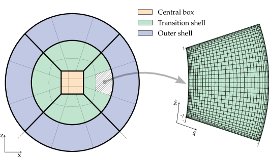
The numerical domain on which we solve the evolution equations in bamps is either a cubed-ball or a cubed-shell grid. Each type is built up of multiple deformed cubes. Each patch is described by two fundamental overlapping charts. In local coordinates and it is a rectangular box . In global Cartesian coordinates and the cubes are transformed and rotated in such a way that when added together they build the desired domain. We give a detailed description in the following. The cubed-ball-grid includes the origin and has a spherical outer boundary. It consists of coordinate patches:
- The central cube:
-
is centered around the origin and ranges from to in the global Cartesian coordinate directions.
- The transition shell:
-
transfers the grid from the inner cube grid to a spherical shell with radius . It contains six patches.
- The outer shell:
-
consists of six patches which extends the grid with additional cubed-shells up to the outer grid boundary at .
The cubed-shell-grid is an excision grid, meaning that it does not include the origin. It is a special case of the cubed-ball-grid, consisting only of the six outer shell coordinate patches.
Cubed-sphere coordinate transformation:
The coordinate transformation used in bamps to construct the grids introduced above relies on the so called “cubed sphere” construction. It was introduced in RonIacPao96 and first applied in the context of numerical relativity in Tho03a ; Tho04 . Since then this idea was implemented in multi-patch approaches PolReiSch11 ; ZinSchTig07 ; SchDieDor06 ; LehReuTig05 . In contrast to many of the earlier examples, the numerical method of bamps does not require overlapping grids, which simplifies the discussion. In RonIacPao96 , the coordinates are constructed by considering great arcs parametrized by equidistant angles. Such angle coordinates are used in Tho03a ; Tho04 ; PolReiSch11 , while ZinSchTig07 ; LehReuTig05 use an intermediate set of coordinates also given in RonIacPao96 that does not have the equidistant angle property. In bamps the latter type of coordinates are employed. The concrete coordinate transformation is the following. First, the local coordinates of each patch are transformed to temporary global coordinates
| (50) |
This patch, which is orientated in positive direction, will later be referred to as the master patch. From here, cyclic permutation is used to rotate the patches to their location in the sphere. The denominator depends on where the coordinate transformation happens. For the patches of the outer shell it is
| (51) |
In the transition shell its definition includes a transition function
| (52) |
This coordinate transformation is constructed to transition from the inner cube to the outer shells. Note that this transformation is uniform along the 3d diagonals, where the distance between inner and outer shell boundary is smallest. This significantly improves the time-stepping restriction in the transition shell.
Subpatches:
Each coordinate patch can be further divided into subpatches. Subpatches are helpful for increasing resolution, and form the backbone of the parallelism of bamps. Each master patch can be split into subpatches with coordinates
| (53) |
with and . In practice we ensure subdivisions are made in such a way that subgrids of two neighboring patches match, and that neighboring patches and subpatches share grid-point positions on their respective boundaries. This is necessary because our current penalty-communication method does not deal with interpolating penalties. Concretely we split the inner cube into subpatches. The transition and outer shell are divided in or subpatches in the radial direction. For the angular direction we choose the number of subpatches to be . In Fig. 1 we show a 2d sketch of the bamps cubed-ball grid subdivided into subpatches.
Discussion:
It is straightforward to specify a mapping between a rectangular master patch and a cubed sphere, although some book keeping for the different patches and different types of shell transitions is involved. It may be useful to examine different such mappings in terms of a numerical quality criterion, say the size of the Jacobian, and to minimize the distortions associated with the coordinate transformation.
III.2 Numerical method
Spatial discretization:
bamps uses the method of lines with a standard ODE integrator to integrate in time. The right-hand-sides are approximated using a pseudospectral method. We use a linear transformation to map the local coordinates of each subpatch into a unit cube . We discretize the subpatch by choosing Gauss-Lobatto collocation points in each dimension, for example,
| (54) |
with , and similarly in the other directions. The number of of grid points depends on the patch location in the grid. The central cube is discretized with points. The radial directions of the transition and outer shell are filled with and points respectively. The number of angular points we chose to be the same as in the central cube to assure that we have matching grids. In Fig. 1 we show on the right the Gauss-Lobatto discretization of a subpatch.
Basis expansion:
On the collocation points we expand all evolution fields in each dimension in a spectral basis using Chebyshev polynomials
| (55) |
and analogously in the remaining two directions. We use the pseudospectral approach and store not the expansion coefficients but the function values at the collocation points .
Derivatives:
The spatial derivatives of the evolution fields are computed by a matrix multiplication. For example in the -direction we have
| (56) |
with the Gauss-Lobatto derivative matrix,
| (57) |
where at boundary points and elsewhere. In practice we do not compute diagonal terms of the derivative matrix by the analytic formulas stated above but use the identity
| (58) |
This negative-sum-trick maps a constant function explicitly to zero and is known to give the derivative matrix better stability as regards rounding errors BalTru03 . In preliminary experiments we found that this gives slightly more accurate derivatives, but have not studied the influence on the accuracy of the simulations presented later in the paper.
Filtering:
We find that a crucial ingredient for numerical stability is the use of a filter against high-frequency growth. For this we follow SziLinSch09 exactly. After every full time-step we apply the filter in each dimension. The filter is easily implemented as a matrix multiplication. For example, in the direction, we filter the function values by,
| (59) |
with the filter matrix
| (60) |
where and and are the Chebyshev synthesis and analysis matrices respectively.
Time integration:
We integrate the fields forward in time using a 4th order Runge-Kutta scheme. Unless otherwise stated we fix the time-step, , with being the minimal Cartesian spatial grid spacing of the whole domain. Empirically we find that this choice for the time step always leads to stable numerical evolutions, in the sense that increasing resolution results in smaller errors. We have not not carried out a stability analysis of the fully discrete system.
BAMPS Octant grid:
When evolving octant symmetric data in bamps, it is possible to only evolve one eighth of the cubed ball grid. This saves computational and memory costs. In the bamps octant mode we choose an odd number of subpatches and a odd number of grid points and reduce the numerical domain to , and . This means that all subpatches containing one of the Cartesian axes are cut in half along them. In these patches we use the symmetry conditions to construct special matrices which compute the derivatives and filters.
III.3 Patching boundary conditions
To glue all subpatches together, we have to impose appropriate conditions at the connecting boundaries of the subpatches. For this we apply the penalty method as is described in Hes00 ; HesGotGot07 ; TayKidTeu10 . The main idea of this method is to add penalty terms for each incoming characteristic variable at the boundary to the right hand side of the evolution equations. We use the characteristic variables of the evolution system to formulate boundary conditions. On the boundary surface we define the outward pointing spatial normal vector . The characteristic variables of the evolution system are given in equation (6) with speeds (7). In vector notation we write
| (61) |
Incoming characteristic variables to the subpatch boundary have positive speeds. On these we want to impose the condition that they are equal to the outgoing characteristic variables of the neighboring patch. Table 1 summarizes all incoming and outgoing characteristic depending on the lapse function and the shift in direction, .
| zero | zero | zero | zero | zero | ||
| incoming | outgoing | outgoing | outgoing | outgoing | ||
| incoming | incoming | incoming | incoming | outgoing | ||
| incoming | incoming | zero | outgoing | outgoing |
As an example, let us now consider the boundary between two patches, patch and patch , and the case . With respect to the spatial normal vector at the boundary pointing outwards of subpatch and inwards in subpatch , the incoming characteristic variables of are the outgoing ones of . In the chosen case, are incoming to L and outgoing of . We want to impose the condition,
| (62) |
Multiplying the first order GHG evolution equations from the left with the matrix of eigenvectors , we obtain evolution equations for the characteristic variables.
| (63) |
Here the again denotes that the similarity matrix stands outside the partial time derivative. At the boundary we now add a penalty to the right hand side of the evolution equation of the incoming characteristic. This is often called weakly imposing the boundary condition,
| (64) |
Afterwards we use the inverse transformation to get back to the evolution equations enhanced with the necessary penalty terms at the boundary. These are also the equations we implement in the code. We treat all six boundaries of the subpatches independently from each other. This means that on the edges we have to consider penalty contributions from two and on the corner from three directions. The size of the penalty parameter can be derived from an energy estimate of the semi-discrete evolution system. This we present in a section IV.
III.4 Outer boundary implementation
At the spherical outer boundary of the domain we use the Bjørhus method Bjo95 ; LinSchKid05 to impose the constraint, physical and gauge conditions given in section II. As for the patching boundaries, we impose conditions on the incoming characteristic to the boundary surface. However, this time instead of adding penalty terms we modify the right hand side of the evolution equations at the boundary in such a way that the boundary conditions are satisfied. We define the outward pointing spatial normal unit vector and use the projection operator to split the principal part of the evolution equation in a part normal and tangential to the boundary surface
| (65) |
Expressed in characteristic variables the normal part is
| (66) |
The matrix is a diagonal matrix containing the characteristic speeds. At the outer boundary we assume that the absolute value of the shift is always smaller than the size of the lapse . This leads to two cases to be considered.
Case :
In this case the incoming characteristic at the outer boundary condition is . According to section II we impose the following boundary conditions, which we give here only schematically:
- 1.
- 2.
-
3.
The physical boundary condition (33),
(69)
Here we labeled principal terms with derivatives tangent to the boundary and non-principal terms with . At the boundary surface we project the evolution equation of the incoming characteristic into the constraint, the physical and gauge part.
| (70) |
All three parts have to be replaced using the boundary conditions. We do this by subtracting the conditions from the bulk right hand side ,
| (71) |
with the special case (35) treated in the obvious way. Transforming back this modified right hand side leads to modified evolution equations at the boundary.
Case :
In this case also the characteristic is incoming. As described in LinSchKid05 , we impose the additional constraint preserving boundary condition
| (72) |
by subtracting it from the evolution equation of
| (73) |
After we have modified the right hand sides at the boundary we transform back to the evolution equations for the primitive fields.
III.5 Code implementation details
Code structure:
The bamps code is written in the C programming language in a modular fashion. The code is designed in such a way that the technical layer is separated from projects for solving physics problems. Inside physics projects we use a Mathematica script, MathToC, which translates equations written in tensor notation into C code. As a standalone program we have developed an axisymmmetric apparent horizon finder, AHloc, which is typically used to search apparent horizons in bamps generated data at the post-processing step. It is also possible to run the finder in a daemon-like mode in which it searches horizons in data of a running instance of bamps. We describe the apparent horizon in subsection V.5.
Parallelization:
bamps is programmed to run in parallel on several computing nodes using the message passing interface (MPI). The subpatches of a bamps grid are distributed on MPI processes as evenly as possible. This means that each process has to handle at least subpatches. As in general the total number of grids is not divisible by the number of MPI processes without remainder, processes have to take care of one additional grid. In practice we choose the number of MPI processes in such a way that the number of processes which have to compute one grid less is minimized.
IV Energy estimate for penalty factor
In this section we derive an estimate for the right choice of penalty factor at the patching boundaries of the bamps domains. The actual technical implementation of the patching condition was already described in subsection III.3. The following calculation is based on the one presented in TayKidTeu10 . However we present it for a general hyperbolic system in curvilinear coordinates, albeit under rather restrictive assumptions.
IV.1 The continuum case
We view the GHG system as a general symmetric hyperbolic system of partial differential equations, but suppress all non-principal terms, and work in the linear, constant coefficient approximation, so we have,
| (74) |
where, in matrix notation,
| (75) |
For clarity we suppress the state vector indices . For this system there is a symmetrizer such that is Hermitian for every unit spatial vector . The energy of the system is,
| (76) |
with the volume form . As discussed in section III.1, each subpatch of bamps has a set of global Cartesian coordinates and a set of local coordinates . The Jacobian transforms between the two charts. To formulate boundary conditions at the patching boundaries which control the energy in the patch, we study the time derivative of the energy, using the evolution equations we replace the time derivatives by spatial derivatives,
| (77) |
In the constant coefficient approximation we can commute the determinant of the three metric in the volume form with the partial derivative and end up a divergence in flat Cartesian coordinates
| (78) |
In the next step we change to the patch local coordinates and ,
| (79) |
Here we have defined and the flux . Now we integrate over all boundary surfaces of the patch,
| (80) |
At a boundary surface, for example , we can write the unit normal vector as,
| (81) |
and split the spatial metric ,
| (82) |
The relationship between the determinant of and the metric in the boundary surface is, We rewrite,
| (83) |
and express the time derivative of the energy as the sum of boundary surfaces integrals over the fluxes ,
| (84) |
The area element is . The fluxes can be rewritten in terms of incoming and outgoing characteristic variables at the boundary surface. The system is symmetric hyperbolic. Therefore the principal symbol has a full set of Eigenvectors which we write as columns of the similarity matrix . With the inverse of this matrix, , we transform the vector of evolution variables to the characteristic variables of the system . The flux expressed in the language of characteristic variables is,
| (85) |
The diagonal matrix contains all the speeds of the characteristic variables
| (86) |
Where we have ordered the characteristic variables in such a way that we group all incoming with positive speeds and outgoing with negative speeds . In this partition it follows that
| (87) |
and with this
| (88) |
If all integrands in (84) are negative semi-definite, the energy of the system does not grow over time. For the boundary conditions we use the ansatz , which means that at the boundary surface we set the incoming characteristic variables equal to a linear combination of the outgoing characteristic variables plus some given data . Choosing the matrix small, we obtain,
| (89) |
The first term only depends on the given data. As we are free to choose it we have full control over this term. The second we can make negative again by choosing sufficiently small.
IV.2 The semi-discrete case
In this subsection we carry out the energy estimate for a semi-discrete system. In our case this means that we discretize the evolution variables in space using Gauss-Lobatto collocation points according to equation (54). The semi-discrete evolution equations are
| (90) |
The energy of this system is defined using Gauss-Lobatto quadrature with the appropriate integration weights
| (91) |
Again we compute the time energy of the system, with , using the inverse product rule to write,
| (92) |
and transform to local coordinates. For this we assume that and obtain,
| (93) |
Using an expansion in Legendre polynomials we can use the summation by parts property to write,
| (94) |
As in the continuum case we introduce the normal outward pointing vector at the boundary and write,
| (95) |
with . We define the flux
| (96) |
and transform it to characteristic variables in the obvious way. This gives us for the semi-discrete case the analogue expression for the time derivative of the energy at the boundary (84). In case of patching the boundaries between two subpatches we apply the penalty method to impose boundary conditions. For simplicity we restrict ourselves to the boundary. For each incoming characteristic variable we add a penalty term to the right hand side of the evolution equations,
| (97) |
with the penalty matrix
| (98) |
and , with the desired boundary data. The time derivative of the energy splits into two parts
| (99) |
The first part is the contribution from the bulk,
| (100) |
The second part changes the time derivative of the energy because of the additional penalty terms in the evolution equation at the boundary,
| (101) |
By inserting the identity into the appropriate places we transform the state vector to the vector of characteristic variables. Then multiplying out the penalty matrix and rearranging leads to,
| (102) |
In total the change of energy at the boundary surface is,
| (103) |
We now consider two neighboring subpatches which we label L (for left) and R (for right). Let us assume they have a common boundary at for the left patch and for the right patch. For each subpatch we can write down the change of energy as in equation (103). As boundary conditions we set the incoming characteristic variables of one patch to be the outgoing one of the neighboring grid,
| (104) |
and demand that the change of energy of the sub patches in time due to the patching boundary is not growing. Sufficient conditions for this are given by,
| (105) |
In bamps we use these penalty parameters, but our discretization is made with Chebyschev rather than Legendre polynomials, the equations we solve are not linear with constant coefficients and nor are the Jacobians mapping from the master coordinates to our global Cartesian coordinates constant. Therefore it is to be determined empirically that the implemented method is in an appropriate sense stable. These facts may contribute to the necessity of employing the filter (60).
V Axisymmetric considerations
Although bamps is a fully 3d code we are often interested in evolving axially symmetric data, which requires special attention for efficient treatment. In this section we collect together the relevant developments undertaken for axisymmetric initial data, apparent horizons and time evolution with the bamps code.
V.1 Brill wave initial data
Brill wave initial data is described in detail in many other sources. For completeness we give a bare-bones summary to highlight the particular choices that we make.
Metric ansatz:
Following Bri59 ; Epp77 , we start from a spatial metric of the form,
| (106) |
in cylindrical polar coordinates, and take the extrinsic curvature to vanish. Note that the assumption of conformal flatness in the - sector of the metric can be made in axisymmetry without loss of generality. Under these assumptions the momentum constraints are trivially satisfied and the remaining Hamiltonian constraint takes the form
| (107) |
We then make the parametrized ansatz,
| (108) |
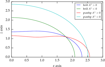
for the seed function and solve for with boundary conditions for asymptotic flatness at spatial infinity. This ansatz is the same as that studied in a number of other studies HilBauWey13 ; Sor10 ; Rin06 ; HolMilWak93 . We call data with geometrically prolate, and that with geometrically oblate. In the initial data an apparent horizon can first be found at with horizon mass . For geometrically oblate data an apparent horizon can first be found at with mass . The pseudospectral method we use to solve the constraints is discussed a little more in section V.4. Our apparent horizon search is explained in V.5.
V.2 Pure plus polarization wave data
Metric ansatz:
Observers distant from a compact object see gravitational waves in the form,
| (109) |
with the wave polarizations and small perturbations of the Minkowski metric. This suggests modifying the ansatz (106) to
| (110) |
so that if we choose the seed function small and centered far from the origin we will have initial data that represents a pure plus polarization gravitational wave. One could similarly make an ansatz for pure cross polarization waves, or indeed make other choices completely like Shi97a which we have also implemented and tested.
The constraints:
Again we start with moment of time symmetry initial data, so the remaining constraint takes the form,
| (111) |
The conformal Ricci scalar is,
| (112) |
and the Laplacian of the conformal metric is,
| (113) |
Once more we impose the obvious boundary conditions for asymptotic flatness at spatial infinity, and choose the seed function,
| (114) |
which makes the conformal metric regular on axis.
Apparent horizons:
Taking centered data with we first find an apparent horizon at around , with mass . Looking for apparent horizons in centered data when , we find the curious result that there is a region in which apparent horizons are first found. Curiously, in the range , the data again seemed to be horizonless. Continue at we find horizons again up to where we stopped our search. We searched for horizons using the resolution . A closer look at the data at the boundaries of the ‘horizonless’ region shows that the shape of the horizon is very nearly not a ray-body, and we expect that our method simply can not find the horizons in this range of amplitudes (see section V.5). We expect that this could be remedied by implementing an offset in in the parametrization of the surface similar to that in which we already have, but we leave this improvement for the future. The first apparent horizon for this data, found at , is plotted in Fig. 2. It has a mass of .
V.3 Teukolsky wave initial data
Initial data for numerical relativity:
Teukolsky waves Teu82 ; Rin08 are an exact solution to GR linearized around flat-space, and were used as a seed function in AbrEva92 , the first numerical study of the critical collapse of gravitational waves, in the construction of full solutions to the constraints. In particular the waves were taken to be centered at some , with a radial width much less than , with an , spherical harmonic dependence, and mostly incoming. Since we are restricting to moment of time symmetry data, we can not satisfy the last of these conditions, but we expect that if the waves are placed at some sufficiently large then they will initially be weakly self-interacting, and roughly one half of the wave will simply propagate outwards. One could use the ansatz made in the Teukolsky wave initial data to construct incoming boundary data, but we leave this for future work. The construction of these data are well-described in BauSha10 and were employed in HilBauWey13 . See also PfeKidSch04 . Therefore here we want only to describe a subtlety that was overlooked in both of these references.
Regularity of the conformal metric:
Let us consider the ‘polar’ Teukolsky data. A similar discussion holds for axial data. The conformal metric for the solution of the Hamiltonian constraint is, in spherical polar coordinates,
| (115) |
with the remaining components vanishing. Here we have already restricted the ansatz by removing terms that vanish for and spherical harmonics. The angular functions and are,
| (116) |
whilst the remaining radial functions are constructed according to the recipe of BauSha10 , so that,
| (117) | ||||
In this expression we have used the shorthand,
| (118) |
and finally the seed function is . In HilBauWey13 the seed function was taken to be,
| (119) |
with . For local flatness however it is necessary Rin06 that the combinations,
of the metric components are regular functions of and . Therefore one may worry about the high powers of present in the recipe. This worry is justified, because for the particular seed function (119) the resulting conformal metric has a conical singularity at the origin, since for example the latter combination diverges like as . Therefore the seed function used in HilBauWey13 is not suitable to construct regular gravitational wave initial data. Regularity is obtained if one chooses instead takes . The fact that such a high power of is required in the seed function illustrates the depth of the singularity that was present beforehand.
Comments on the numerical results of HilBauWey13 with Teukolsky initial data:
Since the seed function (119) gives rise to an irregular conformal metric, the corresponding initial data evolved in HilBauWey13 were in principle wrong, as more careful convergence testing may have revealed. Should we then discard those results? Probably not; since the parameters taken were and , both the seed function and its derivatives were highly suppressed at the origin, and therefore in practical terms it is unlikely that the leading error in the simulations was caused by this problem. We will not attempt however to evolve the older data with bamps, not least because constructing irregular data with our spectral elliptic solver is troublesome. These issues do not affect the seed function used in AbrEva92 which was of compact support.
V.4 Solving the constraints
Compactified coordinates:
To solve for moment of time symmetry initial data, we write the spatial metric in spherical polar coordinates , and compactify the radial coordinate, leaving us with coordinates . The compactification is defined either by,
| (120) |
as suggested in AnsBruTic04 , and used in HilBauWey13 in the same elliptic solver employed presently, or
| (121) |
similar to that employed for example in CalGunHil05 . The parameter partially controls the rate of compactification, but in either case spatial infinity corresponds to .
Numerical solution:
To discretize we employ a Chebyschev discretization in the radial direction, and a Fourier grid in the angular directions. Since the Hamiltonian constraint in this context is linear, solving the constraints amounts to a matrix inversion. With our particular method we find that the choice (120) leads to slightly worse constraint violations at a fixed resolution. One possible cause of this is that the coordinates (120) are irregular at the origin. Perhaps it is possible to use the alternative compactification in the construction of trumpet or puncture blackhole initial data, but we leave this for future consideration.
V.5 Axisymmetric apparent horizons
Formulation of the AH conditions:
An apparent horizon is a closed two surface in the spatial slice, with unit outward pointing normal , with expansion,
| (122) |
where is the unit normal to the surface. Our approach to the apparent horizon search is based on that of AlcBraBru98 as also presented in Tho06 ; Alc08 . First given the spatial metric and extrinsic curvature in Cartesian coordinates, we transform to work in spherical polar coordinates defined by
| (123) |
with and where we take the z-axis to be the symmetry axis. In axisymmetry without twist, the spatial metric and extrinsic curvature then take the form
| (127) |
in the plane. Local flatness on axis implies that the components and are even functions of around the symmetry axis, with around , and similar dependence around . Working in the - plane we may parametrize an apparent horizon by the level set of
| (128) |
in terms of which the apparent horizon condition (122) can be rewritten as a first order ODE system,
| (129) |
for and , where the unit spatial vector and magnitude are given by,
| (130) |
and is the induced metric in the level set. These expressions are evaluated in spherical polar coordinates. As noted elsewhere this parametrization is not completely general, only being sufficient if the apparent horizon is a ray-body containing the point . Regularity of an apparent horizon means that
Search strategy:
Given the metric and extrinsic curvature we go about searching for an apparent horizon in the following way. First we choose and integrate the ODE (129) from to , with initial conditions and . We simultaneously integrate backwards from to taking as initial conditions and . If we have an apparent horizon the forwards and backwards solutions will satisfy,
| (131) |
This gives a non-linear root finding task on the function defined by
| (132) |
One complication is that the ODE system (129) needs to be regularized on the axis to impose our initial conditions. This is straightforwardly done by using the regularity conditions above, resulting in,
| (133) |
at and similarly at . To arrive at this expression we have explicitly used the regularity condition . In our numerical implementation we transform from Cartesian components, so this condition is automatically satisfied and we can instead use the condition in a slightly more complicated form involving and . To the best of our knowledge this regularization of the coefficients has not been used before. The second step of our search is to iterate on until we find a solution, or until the method fails. As an alternative strategy, it is normally proposed to integrate the ODE from to then perform a bisection search on . We were unable to obtain satisfactory results this way because every surface except the apparent horizon itself diverges near , making the bisection hopeless. Reasonable first guesses for would seem to be the position of the maximum of the Kretschmann scalar, or, if an apparent horizon was already found in a previous time-slice, the coordinate center of the previous horizon.
Horizon mass:
In twist-free axisymmetry the apparent horizon mass is related to the area of the apparent horizon as,
| (134) |
We can compute the area of the apparent horizon as a simple integral,
| (135) |
where we have used the fact that apparent horizon is a surface of revolution. Here is the determinant of the spatial metric in Cartesian coordinates.
Simplifying assumptions:
We are often interested in finding apparent horizons centered at the origin in spacetimes that are additionally reflection symmetric about the plane. In this case we can trade our root-finding search above for a bisection search by simply fixing and integrating the ODE (129) from to . Here we start the integration from different initial radii until we find points about which which changes sign. We then bisect in to find the apparent horizon, where . We typically choose the criterion to end the search. As in the more general case, if we find many such surfaces we take the outermost as the apparent horizon.
Numerical implementation:
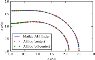
In practice we search for an apparent horizon as follows. During a bamps evolution we output the necessary components of the spatial metric and extrinsic curvature in the plane at different coordinate times. For the integration of the ODE, we use various ODE integrators in the GSL gsl_web . To determine the apparent horizon accurately as fast as possible we use the explicit embedded Runge-Kutta Prince-Dormand (8, 9) method, a high-order adaptive step integrator. When convergence testing we use a simple fourth order Runge-Kutta integrator. To evaluate the metric and extrinsic curvature at each point along the level set we use barycentric Lagrange interpolation inside each bamps sub-grid. For the root-finding we again use the GSL, now choosing one of the ‘hybrid’ algorithms that do not need the Jacobian of the system of equations being solved. In Fig. 3 we present the apparent horizon found using our method for a centered , amplitude , Brill wave initial data set, comparing it with that which we find using a stand-alone apparent horizon finder implemented in the MATLAB initial data code employed in DieBru13 .
V.6 The analytic Cartoon method
Here we discuss the implementation of the so-called Cartoon method AlcBraBru99a for axisymmetry in a pseudospectral method for the Einstein equations. We assume that we are given the 3d system in a Cartesian coordinate system in which all variables are smooth, . The basic idea of the Cartoon method is to apply wherever possible the same coordinates and discretization that lead to stable evolutions in 3d. Hence we compute the axisymmetrically reduced system in Cartesian coordinates and with Cartesian tensor components, without adapting coordinates and thereby avoiding the coordinate singularity at the axis.
Concretely, the computational domain is chosen to be the --plane defined by . Partial derivatives and are computed as for the 3d system. What is missing are the points and the numerical data in the -direction for the computation of . However, we can obtain the -derivative by invoking axisymmetry, since the fields in the , --plane determine the fields for by the rotation symmetry. Similarly, it suffices to consider only the half-plane and while still using the same stencils for and as in 3d.
The Cartoon method was first introduced for a Cartesian BSSNOK BauSha98 ; ShiNak95 ; NakOohKoj87 code using finite differencing AlcBraBru99a . The derivative was computed by adding ghost points in the direction, so that identical 3d stencils could be used for 3d and axisymmetric 2d calculations. For a spectral collocation method, we could do the same and populate a 3d spectral element by rotation. There would still be significant gains in efficiency since only a 2d subset of a 3d spectral grid consisting of many patches needs to be populated. However, it is also possible to derive analytical formulas for in terms of quantities in the plane only, so this is clearly the preferred way to proceed. To our knowledge this was first implemented in Pre04 , in that case for finite differences and the second order GHG system. For an arbitrary smooth tensor , axisymmetry is given by the vanishing of its Lie derivative along the rotational vector, .
Off-axis, .
Let us consider various tensor types of interest, suppressing their and dependence. For a scalar,
| (136) |
The second derivative does not vanish in general. For vectors and covectors (),
| (137) |
the derivative is equal to the components of the vector divided by radius, with and components interchanged. For a symmetric tensor (say, the four-metric ), at , ,
| (138) |
Some components behave like scalars, some like covectors, and some show the two terms occurring in the Lie derivative, which may result in a factor two due to symmetry.
On-axis, .
Axisymmetry by itself does not imply differentiability on the axis. Consider, for example, . We combine axisymmetry with the condition that in Cartesian coordinates in two ways. First, consider parity under , which corresponds to a rotation by around the -axis. Because of axisymmetry, we have and . Since is continuous, the limit exists. Hence for tensors that are even under this type of parity, the derivative vanishes, . For tensors that are odd, the tensor vanishes, , and is a regular, finite value. We therefore impose that vanishes on the axis for even quantities and ask how we can compute the value for the odd quantities.
From vanishing of the Lie derivative, we obtain relations for the tensor components themselves, not for their derivative. For a scalar, there is no extra condition. Examples for relations obtained from (137)–(138) are,
| (139) |
Although we obtain some of the same information that we already discussed for parity, for even parity quantities with two or more indices there are additional relations. For the metric components these are related to covariance under rotation by , or .
To find the derivative at (0,0), we invoke l’Hopital’s rule. Basically, in (137)–(138) the factors become a partial derivative in because the other terms vanish. For example,
| (140) |
Notice that starting with two-index components this is not entirely trivial since there is more than just one term on the right-hand side.
Axisymmetry for partial derivatives of tensors.
There also are objects like , which are not tensors, but partial derivatives of tensors. The Lie derivative is in general not defined for non-tensors, and a priori it is not clear whether implies axisymmetry. However, we can obtain the required formulas by computing
| (141) |
where is introduced to collect those terms that correspond to the Lie derivative of a tensor, and the remaining terms are the deviation from the tensor formula. Note how the last term in provides precisely the term that would otherwise be missing in the sum over index locations in .
The key observation is that in the case of a rigid rotation in adapted coordinates generated by , the second derivatives of vanish,
| (142) |
Therefore, in this special case we obtain the correct result using the tensor formula,
| (143) |
as was also noted in AlcBraBru99a . This generalizes immediately to partial derivatives of arbitrary tensors, and also includes the case of the Christoffel symbol required for the BSSNOK or Z4c system, compare AlcBraBru99a . Eqn. (142) furthermore simplifies the computation of second derivatives.
VI Code validation
In this section we present a set of numerical experiments performed to try and obtain an optimal setup for the first order generalized harmonic system for our gravitational wave collapse evolutions that follow in later work.
VI.1 Gauge boundary
Gauge wave initial data:
We evolve the Minkowski line-element with a perturbation initially placed in the lapse, so that,
| (144) |
In the following set of experiments we always take and , and fix the grid setup. We take the standard formulation used in the SpEC code, namely , and . We impose outer boundary conditions at a coordinate radius of and evolve in 3d with octant symmetry imposed.
Harmonic gauge:
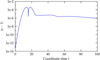
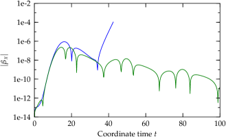
Starting with the pure harmonic gauge , we find that the outgoing gauge wave is harmlessly absorbed using either the gauge boundary condition (35) or (36). At the particular resolution and grid-setup that we chose for this test the harmonic constraint violation at the end of the evolution, , is around and shows no sign of increasing with either choice of gauge boundary condition. The difference between the results with the two gauge boundary conditions is rather small, the maximum difference in the shift being around at the end of the run. But here the initial pulse is very weak, and this is of no concern. In the left panel of Fig. 4 we plot in the outer boundary, to demonstrate how the coordinates settle down.
Generalized harmonic gauge:
Switching now to use the generalized harmonic gauge condition (14) with and . Using then the gauge boundary condition (35) we find that the shift starts to grow at the boundary, and the numerics fail at . This behavior is perhaps not surprising given the large damping coefficents and the understanding obtained for the constraint preserving subsystem with damping in section II.2. The gauge source functions have the same effect on the gauge as the damping terms on the constraints, namely they cause reflections from the boundary. We expect that it will be suppressed as the outer boundary is placed further out so that the gauge sources are smaller where the boundary condition is applied. Using instead the gauge boundary conditions (36) this growth is completely absent, which is why we do not implement conditions derived explicitly to reduce gauge reflections in the present work. This behavior is demonstrated in the right panel of Fig. 4 where one sees the magnitude of the shift vector in the outer boundary in each case. With the gauge boundaries (36), at the end of the run the harmonic constraint violation is around and appears not to be growing. Looking at the shift however, it does seem that some further improvement may be possible in the future, as its peak lies at the outer boundary, with a value around .
VI.2 Constraint experiments
Simplified subsystem:
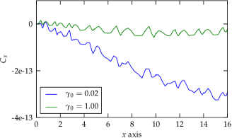
We now repeat some of the experiments of the previous section with the choice , and with different choices of , using always the gauge boundary condition (36). With the pure harmonic gauge , we find that the constraint violation at is again around if we take , and slightly larger, but still less than if we choose , the value suggested by the experiments in WeyBerHil11 for a related formulation. Moving to the generalized harmonic choice (14) once more, we find that again that the violation at the end of the experiment is of the same order as when using the pure harmonic gauge. The result is plotted in Fig. 5. These results may not be representative when evolving different initial data, but we cautiously take and as our default setting, periodically testing different choices, most often playing with in such experiments.
Constraint preserving conditions:
We performed the same experiments, with the generalized harmonic gauge and the new default formulation parameters, changing to the alternative constraint boundaries (43) or (49) and found first that the violation throughout is very similar to the initial choice (32). Although initially the violation with the reflection reducing condition is slightly smaller than with the ‘geometric’ condition, later on there is practically nothing to choose between them. Considering that the violations are in the round-off regime it is hard to judge from this experiment which of the conditions behaves most favorably.
VI.3 Lapse power in constraint damping
Initial data:
We now evolve centered Brill wave initial data, which is subcritical, with an ADM mass of . We evolve on the same grids used in the previous section, but with a slightly higher resolution ( rather than points per cube). We evolve using with , the standard choice elsewhere, or , a modification which we hope will reduce constraint growth in the strongest field region. As above we use the generalized harmonic gauge (14). We use only the gauge boundary condition (36).
Basic dynamics:
The Kretschmann scalar initially has a peak at the origin, evaluated around on the bamps grid, slightly less than in the previous study HilBauWey13 . This peak oscillates at the origin, peaking after an initial bounce with value around . The feature then rapidly propagates away and by a coordinate time , the peak value on the grid is less around . The lapse initially decreases at the origin, this feature then propagating out to the outer boundary, behind which the lapse drifts back towards its initial value, unity.
Constraint violation:
Examining the constraint for the data along the -axis, we see that only very small differences in the constraint violation between the and evolutions. The small differences are not surprising because the lowest value the lapse function takes is around having started from . The peaks of the constraint in the evolution are about - smaller than in the run. Increasing the amplitude of the initial data to , one might expect the improvement to be more significant as the lowest value of lapse decreases to , but the difference still amounts to between - at the peaks of the violation.
VI.4 BAM vs. bamps comparison
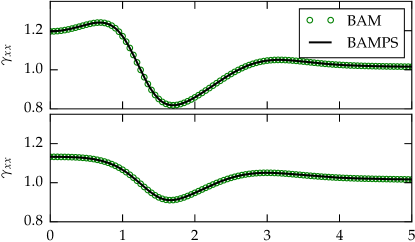
Another validation strategy for bamps is to compare the numerical results with those of an independent code. For this we used BAM BruGonHan06 , evolving identical initial data with the same gauge conditions. This comparison we performed by evolving a centered Brill wave with . We chose this weak amplitude because evolving the Brill data accurately with BAM rapidly becomes expensive as increases in magnitude. We used pure harmonic slicing with either harmonic shift or the damped harmonic shift . In the BAM code we evolve with the BSSNOK formulation, for completeness, this gauge condition is given by
| (145) |
in terms of the conformally decomposed BSSNOK variables. For this test we did not employ the spherical shells or constraint preserving boundary conditions of HilBerThi12 . Since the outer boundaries were placed at , the solutions to the continuum PDEs being solved are not identical. Therefore we should not hope for perfect agreement for long. In Fig. 6 we plot the spatial metric component at , when the agreement is still very good for either choice of the shift, being practically indistinguishable by eye. In practice the main source of disagreement at the resolution of these runs comes from mesh-refinement boundaries in the BAM grid setup.
VI.5 Octant and Cartoon
Initial data and grids:
To test our implementation of symmetry reduced expressions, either octant, Cartoon, or their combination we evolve weak centered pure plus polarization initial data as described in section V.2, using once again the generalized harmonic gauge (14) and the gauge boundary condition 36. We started with a base cubed sphere 3d grid with points per direction, and the number of subpatches derived from and . The outer boundary was placed at in the units of the code. For ease of comparison, the breakdown of the grids was:
| 3d | |||||
|---|---|---|---|---|---|
| octant | |||||
| Cartoon | |||||
| cart. oct. |
where the numbers in parentheses denote the number of those grids that were cut in half (at the axis) once, twice, or three times respectively, for the 3d grids, and once or twice for the Cartoon grids. Note that our current non-octant Cartoon implementation is not optimal because we evolve the whole - plane, wasting effectively a factor of two. Currently we use the code most often in Cartoon octant mode, so fixing this does not have a high priority. Looking at the table the main observation is that the expected reduction factor of eight (four) in the total number of grid points is present between the 3d (Cartoon) and octant grids, but that this number is not so closely reflected in the grid breakdown, where we get only a factor six (three) in the total number of grids. This is obviously because there are many grids with fewer points. Since our parallelization does not take this fact into account, it is possible that one MPI process is given all non-cut grids, and so we can expect that the speedup rate is determined to a large extent by ratio in the number of grids. As we make the domain larger the relative number of cut grids decreases, so we might expect that asymptotically the full speedup factors of eight or four can are attained.
Basic dynamics:
Although irrelevant for the octant Cartoon comparison, since these data have not been used before, we give a brief description of their evolution. Initially the peak of the Kretschmann scalar occurs at with a value . This profile then oscillates about three times at the origin, attaining a peak value of before rapidly dispersing. Looking at the lapse we see the familiar behavior that at the origin it oscillates slightly before presenting a longer decrease, although at the minimum is only , having started from everywhere. Afterwards this pulse propagates out, roughly following the disturbance in the Kretschmann. Looking at the shift component along the -axis we find that early on there is a growth which peaks at , with value . The development of the shift looks more like a slowly oscillating standing wave than a localized propagating feature.
3d, octant, Cartoon and octant-Cartoon comparison:
Taking first the 3d and octant evolutions, we see near perfect agreement throughout the evolution. There are small differences however, starting from the beginning of the simulation at the level of round-off; differences of in metric components, which slowly drift as the evolution goes on. This behavior is expected because the derivative approximation differ at this level. Similar differences were found between the other setups. These differences are never larger than the constraint violation, in for example , and we have looked at convergence (see section VI.6 for more discussion) with each setup, although not for this data, and find no indication of a problem. For the speed comparison we ran the code with each setup on 24 cores (with hyperthreading) of our local cluster Core12 with Intel Xeon X5650 processors. The octant run was a little more than times faster than the 3d run, as expected given the foregoing discussion. The octant Cartoon run was about times faster than the pure Cartoon test, which is a little disappointing. Going from to radial subdivisions in the outer shells, this value increases to , demonstrating the expected dependence. Comparing the full 3d and octant Cartoon runs, there was a gratifying speed up of nearly a factor .
VI.6 Convergence
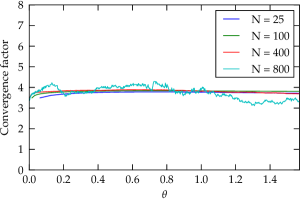
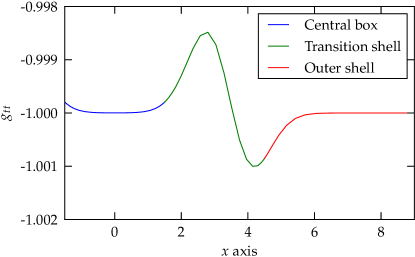
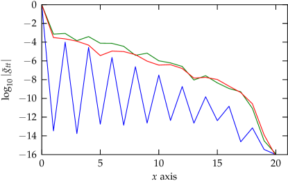
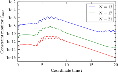
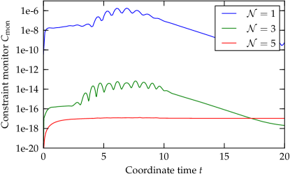
The bamps numerical method gives us two options for increasing resolution. The first is to add grid-points in every domain, the second is to subdivide grids further, keeping the number of points inside each subpatch fixed. Given fixed finite computational resources it is not obvious what is the optimum strategy to achieve the smallest possible error, because although we would expect that adding points brings spectral convergence, it also comes with a dependence in the allowed time-step, whereas on the other hand, as we will see, adding more subpatches allows the code to scale up to a large number of processors. Probably the optimal strategy relies on a balance between each. To examine the effect of each strategy in the simplest possible way, we evolved gauge wave initial data on the Minkowski spacetime, which was setup by choosing , , with as usual, and otherwise the flat spatial Cartesian metric and vanishing extrinsic curvature. The results are plotted in the four panels of Fig. 7 and confirm our expectations.
VI.7 Filtering
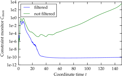
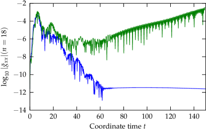
To demonstrate the necessity of the filter (60) we evolved a centered Brill wave. The results are plotted in Fig. 8. In the left panel we see that without filtering the constraint violation starts to grow exponentially in time, whereas with filter the growth is completely absent and the norm of constraints remains steady at a very low value. In the right panel we plot the magnitude of the fourth highest spectral coefficient of in the transition shell as a function of time. This coefficient is the first that is directly unaffected by the filter. We see that the growth in the constraints seems to be associated with an explosion in the higher spectral coefficients. Interestingly we tried the same experiment with gauge wave initial data, and did not see the effect, at least in the same time-frame. We expect that the same behavior would manifest if we were to evolve long enough. The obvious conclusion we draw from this is that it is important to test these methods with several data types to get a reliable picture of their properties.
VI.8 Performance
Strong-scaling:
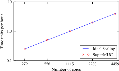
The current bamps parallelization strategy is to obtain perfect scaling using many subpatches, and splitting these subpatches across many processors. The key is that, contrast to buffer zones required in the decomposition of a finite differencing grid, only d surfaces of points need be passed by network communication, making the relative time spent there negligible. In a finite differencing approach the relative size of the buffer zones decreases with resolution, but in practice can still be significant in production runs. In Fig. 9 we present strong scaling plots performed on the SuperMUC cluster located in LRZ Garching, with Intel Xeon E-C processors. We ran the code in d. We took a grid with total subpatches, and increased the number of cores used until we were computing one patch per core. We find perfect scaling. On the other hand bamps is currently not parallelized whatsoever at the subpatch level, which means that the maximum number of points per subpatch is in principle determined by the amount of memory available to one core. At least when running the code in Cartoon mode however we do not find, in practical terms, that this is problematic. Instead the restriction in the time step makes increasing the number of points infeasible long before we are close to filling the available memory. In d this may no longer be the case. We leave such considerations for future work.
VII Single blackholes
The main thrust of our development has been towards treating collapsing axisymmetric gravitational waves accurately. For super-critical data the cubed-ball grid is unsuitable after the formation of an apparent horizon. Therefore the strategy for long-term evolution is to take the data and interpolate onto a cubed-shell grid, with the excision surface suitably positioned, changing the lapse and shift to be sure that the excision surface is a true outflow boundary. A necessary requirement is to treat a single blackhole, which is what we discuss here.
VII.1 Initial data
Kerr-Schild coordinates:
We evolve the Schwarzschild solution in Kerr-Schild coordinates as was done with an earlier version Bru11 of the present code. Although the current numerical method is not particularly close to that used previously, some components of the older code were inherited. Importantly evolving this data allows a simple comparison with the previous method and results. In spherical polar coordinates the metric and extrinsic curvature take the form,
| (146) |
with the flat metric on the two-sphere, and
| (147) |
respectively. Inside the code the line-element is written in Cartesian coordinates in the standard way. More discussion of Kerr-Schild coordinates can be found in Coo00b ; MatHuqSho98 .
Harmonic Killing coordinates:
We additionally evolve starting from the harmonic Killing slicing described in CooSch97 , which serves as a convenient starting point when transitioning from one generalized harmonic gauge to another. For this initial data, in spherical polar coordinates, the metric and extrinsic curvature are
| (148) |
and
| (149) |
with the remaining components vanishing. For this data spatially harmonic coordinates are obtained by building Cartesians according to,
| (150) | |||||
The resulting metric has a coordinate singularity at , with implicitly defined in the obvious way from the new coordinates. The coordinate singularity is not a principle problem as we could just put the excision surface outside this radius. But bamps relies on standard Cartesian coordinates in several places. So in the code we could transform in the standard way but then choose the gauge source function,
| (151) |
with the Jacobian between the standard -index Cartesians and harmonic Cartesian index coordinates (150), the compound object is defined by,
| (152) |
with and where indices are manipulated in the obvious way with to obtain (151). Instead we just choose the gauge source function to be fixed at its initial value, as will momentarily be discussed. In this section we use the code exclusively in Cartoon mode, on a cubed sphere grid. We start with the excision surface at , and the outer boundary at . In our base setup we take radial subpatches each with points per direction. The runs were performed on a desktop machine with an eight-core intel i7 CPU, which was able to compute at about , the base run requiring about MB of RAM.
VII.2 Freezing gauge source functions
Killing gauge sources:
Given initial data which admit a time-like Killing vector, we can ensure that the evolution of the system is trivial, at the continuum level, neglecting the effect of outer boundary conditions, by choosing the Killing lapse and shift, and taking the gauge source functions so that initially. In particular we must choose,
| (153) |
Kerr-Schild evolutions with SpEC GHG:
We began by evolving the Kerr-Schild initial data with the standard formulation parameters of LinSchKid05 , namely and on our base grid as just described, using the gauge boundary conditions (35). Immediately we see that the innermost subpatch has the largest constraint violation, peaked at around in the component of the harmonic constraint. This is not surprising because the innermost subpatch contains the part of the solution with the largest derivatives. The evolution successfully continues until the final time . But after the initial expansion to , a slow expansion in is visible, and this growth becomes more rapid as the simulation continues. By the end, the maximum value of is around , with peaks appearing at the inner and outer boundary of roughly the same size. We then increased resolution from the base grid to and . The point grid runs at about , and the initial peak in the constraint violation is reduced by a factor of about two, with this ratio of improvement slowly declining until the end of the evolution. The grid runs at , with both the initial magnitude of the violation and the ‘slow expansion’ of the constraint quashed, the peak being a factor smaller than in the base run at the end of the simulation. The highest resolution point grid ran at , with the final improvement in against the base run being a factor of . Since the largest constraint violation occurs in the excision subpatch an obvious question is whether or not the excision and outer boundaries would interact badly if they were on the same grid. Although the issue is of little practical concern for production runs, for development it deserves a little attention, and therefore we evolved our base grid from before, but cutting the outer two subpatches so that the outer boundary lies at . This test is not completely fair because the outer boundary conditions are expected to perform better as they are applied further out. We find that the initial peak in the violation of the constraint is about five times greater than in the base run at . At the end of the evolution again at by coincidence the constraint violation in the restricted domain is smaller, but this is just because the slow oscillations in each simulation are out of phase.
Kerr-Schild incoming wave evolutions with SpEC GHG:
Next we evolved the same initial data and gauge, but this time with the same domain as in Fig. of LinSchKid05 . To do this we took radial subpatches, with the same base resolution as before, so that the outer boundary is placed at . We similarly specify exactly the same given data for an incoming gravitational wave as in that study, taking in particular,
| (154) |
with the vectors here the coordinate vectors defined in the obvious way. We take,
| (155) |
with , and . In Fig. 10 we show the results from these experiments, obtained with a sequence of different resolutions. We plot the Weyl scalar (28), averaged over the outer boundary,
| (156) |
The surface area of the outer boundary is . Fitting the highest resolution data between and we find a ring-down frequency of as expected ChaDet75 . In this evolution we found that the apparent horizon oscillates slightly as the gravitational wave is absorbed, increasing the horizon mass (134) by about , with the ADM mass of the analytic initial data. Note that the gauge boundary condition being employed here is not identical to that used in LinSchKid05 , so the agreement is remarkable. The effect of much larger pulses of gravitational radiation falling onto a blackhole using similar gauge conditions was studied in ChuPfeCoh10 .
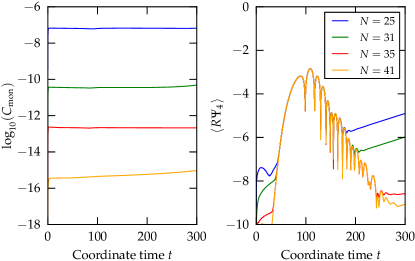
Discussion of and comparison with Bru11 :
The prior bamps study focussed on obtaining numerical stability in the evolution of a single Schwarzschild blackhole with the Kerr-Schild slicing. The numerical method used a Chebyschev-Fourier-Fourier spatial discretization on a single shell with a spin weighted spherical harmonic filter to prevent high frequency growth of the error. In that study the outer boundary condition employed simply fixed the incoming characteristic variables (6) to some given data, namely their initial values. This approach is possible only when the analytic solution is known, otherwise incoming constraint violations are generated. Placing the inner boundary at and the outer boundary at , very long evolutions, say until at least , could be performed with little resolution, in accordance with LinSchKid05 . On the other hand, using this method, the naive boundary conditions rapidly deteriorated as the outer boundary was pushed out, and, crucially resolution did not help but rather made the problem worse. A possible explanation for the latter effect is that no filter was being applied in the radial (Chebyschev discretized) direction, which have already seen is a crucial ingredient for stability with the current method. The likely cause of the boundary problem is that, as explained in RinLinSch07 , boundary conditions that just freeze the incoming GHG characteristic variables are orders of magnitude more reflecting than the Sommerfeld like choice contained in (35). Evidence for this is obtained in the current code by changing from the gauge boundary condition (35) to use instead,
| (157) |
evolving once more the Kerr-Schild initial data on the base grid. Placing the outer boundary further out then results in greater reflections. However rather than trying to improve a condition only suitable for evolving known data, we immediately moved to the constraint preserving, radiation controlling conditions, with which this issue is completely absent. The first attempted implementation of a regular center in the bamps code was to use the Chebyschev-Fourier-Fourier discretization with a double covering in the radial direction, similar to that employed in Tre00 . The approach was not successful, as we always eventually found irregularities in the numerical solution at the origin. An exponential filter was applied to the Chebyschev coefficients in the radial direction, but to little effect. Eventually we settled on the cubed sphere approach, in part because of the expectation that they will later be more convenient for mesh-refinement. Other possible solutions to the problems we faced would be to use one-sided Jacobi polynomials as in SpEC MuhNouDue14 or to employ a filter that projects the solution in another basis onto these polynomials.
Kerr-Schild evolutions with simplified constraint subsystem:
Using our standard choice for the formulation parameters , and taking , returning to our base resolution from the tests with the SpEC version of GHG, we find that by the constraint is about times larger than that we obtained before, and by the end of the simulation the new run has accrued a constraint violation with a sharp peak at the outer boundary of order . This result seems to be in contradiction to those of section VI.2, until we remember that there the gauge boundary condition (36) was employed. Increasing the constraint damping to , the initial violation is comparable to the SpEC GHG evolution previously described throughout the evolution, and the spike at the outer boundary is suppressed by roughly an order of magnitude. At the end of this run the maximum of the constraint occurs at the excision boundary with a value around . This experiment thus highlights that the choice of the damping parameters and boundary conditions can be rather subtle.
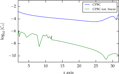
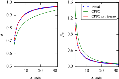
Kerr-Schild evolutions with alternative boundary conditions:
Next we returned to the base grid, and switched to the alternative gauge boundary conditions (36), with and . We find that the aforementioned growth in the constraints is completely eradicated, and the drift in the lapse and shift is also suppressed. Evolving the same data with the same formulation and gauge boundary condition, but using the modified constraint preserving boundary condition (43) gives almost identical results. Using instead the reflection reducing conditions (49) we see a small improvement in the violation throughout the simulation. Repeating the experiment with the incoming gravitational wave injected through the boundary with the standard constraint preserving condition (32) and the gauge boundary conditions (36), the growth visible in Fig. 10 is also completely absent, even on the base resolution grid.
Harmonic Killing slice evolutions:
We now returned to our base grid and resolution, taking the formulation parameters , and , evolving the Harmonic Killing slice with the gauge boundary condition (35). The test successfully runs to . Comparing with the equivalent evolution of Kerr-Schild data, we see that initially near the excision boundary the constraint violation is significantly greater in the Harmonic Killing test. By this difference has accrued to around two orders of magnitude. Later however, as the violation in the Kerr-Schild Killing evolution starts to grow, it overtakes that of the Harmonic Killing evolution. At the peak of the constraint violation in the Harmonic Killing run is about an order of magnitude smaller than in the earlier test. As remarked before, in the Kerr-Schild test the inner and outer boundaries have roughly the same magnitude in the constraint violation. Interestingly the twin peaks are not present in the Harmonic Killing data because the outer boundary is hugely improved. This finding is consistent with the gauge wave tests presented in section VI.1, although this test is somewhat easier for the gauge boundary conditions because of the complete lack of dynamics present in the gauge wave test. In the Harmonic Killing evolution we are evolving with pure harmonic slicing, and some non-zero spatial gauge source functions, which suggests perhaps that the growth at the outer boundary is predominantly caused by the use of a non-trivial gauge source function for the lapse function, as it interacts with the boundary. Indeed looking once more at the lapse function towards the end of the Kerr-Schild evolution we see that it is drifting from its initial value, but that this effect converges away with resolution. In any case, the peak in the constraint violation at the outer boundary in the Killing Kerr-Schild data is suppressed as the outer boundary is placed further out.
Harmonic Killing slice with gauge perturbation:
A desirable property for a set of dynamical coordinates is that in the presence of a, perhaps approximate, timelike Killing vector they quickly asymptote to a time-independent state. For an arbitrary physical or gauge perturbation there is no hope that this will occur, and nor can any finite set of numerical experiments prove that that there is a basin of attraction to a stationary state. We can however look for some indication of this behavior. To do so we start by taking the initial data for the Killing harmonic coordinates, and then perturb the initial lapse function by Gaussian as in the previous gauge wave evolutions. In terms of the first order GHG variables this is a slightly fiddly procedure, as compared with the use of lapse, shift and spatial metric, so we give a quick summary:
-
•
Set spatial metric and extrinsic curvature from the exact solution.
-
•
Take the Killing lapse and shift. Use the conditions and to set the gauge source functions .
-
•
Add the desired perturbation to the lapse (or shift) and then transform to the first order GHG variables.
We perturbed the lapse by a Gaussian,
| (158) |
with and . A similar experiment was made in LinSzi09 , but starting from a Maximal slice of Schwarzschild to test the gauge driver system. We find that the perturbation in the lapse propagates away, rapidly leaving behind the solution with the harmonic Killing data with unperturbed spatial coordinates, or at least negligibly perturbed. The greatest danger to the evolution is probably that the excision boundary fails to be outflow, but at least with this perturbation that does not occur.
Harmonic evolutions with incoming gravitational wave:
Giving the same gravitational wave data (154) as previously, evolving with the standard boundary conditions (32) and (35) but using the harmonic Killing gauge source functions. It is not obvious how, if at all the spacetime computed is related to that considered before, but in any case we find a very similar decay in . Remarkably the growth present in Fig. 10 is absent even in this low resolution test.
VII.3 Phasing-in the damped wave gauge
The transition function:
As elsewhere, we follow SziLinSch09 to transform from one generalized harmonic gauge to another . The composite source function is simply,
| (159) |
The transition function is,
| (162) |
In the following experiments we choose and . Note that care must be taken to construct the time and space derivatives of with the transition function. This choice results in gauge source functions that are only at , which could be avoided with a different transition function. It is not clear if this finite differentiability will have a large effect on extracted physical quantities from a simulation.
Kerr-Schild initial slice:
For our first phase-in test, we started with the Kerr-Schild slicing of Schwarzschild and evolved with and , on our base resolution grid. We took the gauge boundary condition (35) and the constraint preserving condition (43) (including a term). We used the wave gauge parameters and . The value of here is much smaller than in our wave collapse evolutions. The reason for this is that when evolving a blackhole it is crucial that the excision boundary is pure outflow in the PDEs sense. In other words the characteristic speeds must all have the same outward pointing sign. Since the speeds in the direction are like this means that the shift can not become too small or else the excision boundary will fail, which in turn means that can not be chosen too large. We therefore place the excision boundary deeper into the blackhole so that and carefully monitor the coordinate lightspeeds at the inner boundary. Note that this requirement is likely to cause difficulties when computing extreme gravitational waves, because on the one hand large shifts can result in poor resolution of important features, but on the other they may be required in some other region so that we may successfully excise the blackhole region. In the evolution we immediately see significant dynamics and that for example the peak of the constraint violation along the -axis is two orders of magnitude greater than in our initial Kerr-Schild base run with Killing gauge sources. The reason for this is presumably the presence non-trivial dynamics, plus the fact that we are excising nearer the physical singularity similar to the effect we saw with the harmonic Killing slice. Regardless, by the data seem very close to stationary. The simulation then evolves to the target time , and remarkably at the end of simulation the constraint violation in along the -axis has a maximum value which is an order of magnitude smaller than in the base run. At no point does the excision boundary fail to be outflow. As a check of the axisymmetric apparent horizon finder we compare the results obtained with the simpler algebraic condition,
| (163) |
which characterizes the position of the apparent horizon in spherical symmetry. We find near perfect agreement throughout. The apparent horizon moves from its initial radius inwards until it reaches around . From there the horizon starts to grow again and seems to settle down to . However in our lowest resolution run, a small drift of the horizon outwards is visible. At late time of the simulation, around , this drift accelerates and we observe that the horizon becomes aspherical. Higher resolution runs show that this effect converges away.
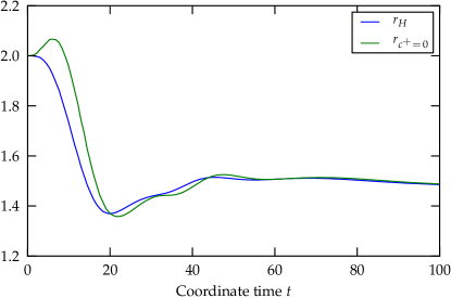
Harmonic initial slice:
Since the stationary fully harmonic coordinates are singular at , one might guess that the stationary spatial generalized harmonic coordinates with gauge source functions (14) are also singular at some radius on the Killing slice, at least for some range of the parameters . Given the broad experience in using these coordinates in binary blackhole simulations, the naive expectation would be that, if present, this coordinate singularity is pushed further towards the physical singularity rather than out towards the event horizon for standard choices of the gauge source functions. But this behavior is not clear. To truly resolve the issue one could simply solve for such coordinates along the lines of HanHusPol06 , but this we defer for the future. Instead we performed simulations varying the initial excision surface from the base grid excision radius down to in steps of . Unsurprisingly we find that initially the constraint violation, is greater in the excision subpatch as the inner boundary is placed closer to the singularity, amounting to about an order of magnitude in the constraint between the and boundary runs by . Besides this there is little to distinguish between the five runs, and at least down to this excision radius no sign of a coordinate singularity forming. By eye the lapse function in the shared part of the domain agrees very well throughout the evolution. Although a slight drift between them is present towards the end of the test, this is acceptable since the outer boundary conditions are being imposed at different radii, the solutions need not agree everywhere. There is however a time around above which the runs with inner boundary fail to be outflow at the excision surface. Assuming that this is not caused by numerical error this means that boundary conditions are required at the surface. It furthermore means that convergence of the numerical scheme as resolution is increased is impossible. The fact that this does not correspond to a catastrophic failure of the code is inconvenient, because it indicates that great care must be taken in monitoring the excision surface. On the other hand, since placing the excision boundary very far in has a large cost in accuracy, a careful balance must be struck. In the SpEC code this is taken care dynamically of by a control mechanism HemSchKid13 ; SchGieHem14 which bamps does not yet have. In Fig. 12 the relationship between the character of the excision boundary and the apparent horizon is examined. Comparing the initially harmonic and Kerr-Schild slice evolutions with excision radius we find that although the lapse functions initially disagree, by about they have exactly the same profile and lie almost on top of one another. After this time the agreement is maintained.
VIII Evolution of Supercritical Waves
In this section we present the numerical evolution of a centered Brill wave, see section V.1, with . This highly supercritical initial data is used as a test case for our excision algorithm for a dynamically forming blackhole.
VIII.1 Dynamical excision strategies
Our dynamical excision method currently consists of the following steps:
1. Evolve to collapse: Evolve on cubed ball grid, running the apparent horizon finder in ‘daemon’ mode. The finder then triggers a bamps checkpoint once a horizon is found.
2. Go-to excision grid: Next interpolate the checkpoint data onto a cubed-sphere grid. In this step we want to place excision boundary just inside the apparent horizon, but as we have already seen in the single blackhole evolutions this may not always be possible, as some wiggle room is needed to allow for dynamical behavior of the horizon. This can require some experimentation, although fine-tuning does not seem necessary.
3. Regauge: Adjust the lapse and shift to ensure that the excision boundary is pure outflow. As a particular choice, we take lapse and shift from Kerr-Schild slicing of Schwarzschild,
| (164) |
and translate to Cartesian components in the obvious way. It is desirable that the radial coordinate light-speeds are close to zero, preferably positive, at the apparent horizon, since this determines the direction of motion of the horizon. Therefore we choose the parameter to satisfy this condition reasonably well, although again without particular fine tuning.
4. Safety-net evolution: We then use single blackhole gauge source parameters like and . During the evolution we use a safety net. If any coordinate light-speed on the excision boundary reaches a given threshold, typically we again regauge to guarantee the outflow character is maintained. We monitor the apparent horizon, and if it falls off of the numerical domain we return to an earlier checkpoint, regauging with a smaller to avoid this behaviour. As the horizon expands we monitor the position and periodically return to the Go-to step above, excising further out and regauging with a greater .
Discussion:
As currently implemented this procedure requires that some steps be performed by hand. The numerical results in the following subsection serve to demonstrate ‘proof of principle’ of this algorithm. On the other hand it seems at least clear how those steps should be automated. At the regauge step the use of the first order GHG variables is again a little fiddly. Much more convenient would be if the lapse and shift were readily available as variables. But the procedure is similar to that described in the gauge perturbation tests in section VII.2, so we do not give full details. Also at the regauge step, it might be good to choose lapse and shift by abandoning the spherical ansatz and imposing that the coordinate light-speeds at the apparent horizon vanish. The SpEC approach to controlling the excision surface is much more sophisticated, employing a control mechanism HemSchKid13 , we hope to avoid that investment in the near future. Because we are interested in the collapse of waves to form, presumably, a single blackhole it seems reasonable to use a simple approach if at all possible. One aspect of the method that is not very aesthetically appealing, is that by changing the lapse and shift in discrete steps we are computing a spacetime, or patch of spacetime in coordinates that are not globally smooth. Another issue associated with this is that of geometric uniqueness, which for the IBVP is an open question. Nevertheless one expects that the differences to the computed spacetime with one choice of regauging parameters or another will be rather small in practice, so this does not represent an immediate practical concern.
VIII.2 Supercritical Brill wave evolution
Initial data and grid setup:
We evolved a centered Brill wave as described in section V.1, with seed function (108). We chose a centered wave with . The ADM mass of this initial data is . The maximum of the Kretschmann scalar in the initial data occurs at the origin, taking the value . Following the algorithm just outlined, we began on a cubed-ball grid with , and points per cube, with internal boundaries , and the outer boundary placed at . We ran the code in Cartoon mode on our local cluster Quadler with cores. We evolved with the generalized harmonic gauge, as in section VI in the evolution of a much weaker Brill wave, now with the gauge parameters and . At coordinate time we first found an apparent horizon with mass .
Continuation to code crash:
If we continue this evolution without going to an excision grid after the apparent horizon forms, we find that the constraints inside the apparent horizon rapidly grow along with the Kretschmann scalar. The run then crashes at roughly . This gives the clear signal that if we are to examine the final masses of blackholes formed during collapse, using the GHG formulation, a robust excision algorithm will be essential. In fact at the horizon has a mass of on the cubed-ball grid, but at the end of our excision simulation, to be described momentarily, we find that after apparent horizon formation it has mass . In the first critical gravitational wave collapse paper AbrEva92 , the blackhole masses were evaluated roughly after apparent horizon formation, according to a prescription based on the quasinormal modes of Schwarzschild. Comparing those values with ours is difficult because we use different time coordinates, but the basic expectation is that the Maximal slicing condition is more “singularity avoiding” than one of our generalized harmonic gauges, and therefore we might expect to obtain comparable results if we can evolve for a similar coordinate time after the appearance of a horizon. This is, however, not clear and deserves further investigation. In any case without excising the blackhole region, the meager after collapse is clearly insufficient. We have seen in HilBauWey13 that with the moving-puncture method this type of data also did not result in successful evolutions beyond apparent horizon formation. But here at least a concrete improvement has been made, in that we find an apparent horizon before the method fails!
Evolution on excision grid:
Checkpointing the solution at we then interpolating, again with barycentric Lagrange interpolation as used in the apparent horizon finder, onto a cubed-sphere grid with excision radius at with the outer boundary position fixed, and with with angular patches, now with points per cube, naturally again evolving in Cartoon mode. In the regauge step we choose here . This step immediately removes most of the constraint violation from the computational domain, and the largest spatial derivatives, so that the constraint monitor is as compared to on the original cubed-ball. This difference seems very troublesome until we take into account that, for example the peak of the Kretschmann scalar on the cubed ball grid is whereas on the cubed sphere it is . So the reduction in the constraints obviously occurs because we are removing the most extreme part of the domain. Note also that our definition of the constraint monitor does not include a normalization by the size of the solution, as in for example LinSchKid05 and subsequent papers. In view of this our reduction in resolution is justified. The evolution then proceeded, now on cores using . The regauge safety-net was triggered times up to , having fixed , but the apparent horizon remains on the computational domain throughout the calculation. At we perform the “Go-to” step of our algorithm again, this time excising at choosing . After this the regauge safety-net was not called before , when we changed cubed-sphere grid once more, keeping the same grid parameters but excising at , and regauging with . The evolution continued , at which time we changed grid for the final time, before which the safety-net was again not called. In the last grid we took the excision radius to be and regauged with . After this the regauge safety-net was not called, and the evolution was terminated at after apparent horizon formation. Note that in this evolution the “Go-to” step also employed the phase-in for the generalized harmonic gauge, as described in our single blackhole evolutions in section VII.3, taking the same parameters employed in those earlier tests, but now with the initial source functions chosen so that the lapse and shift were frozen as the evolution starts on the new grid. Other experiments show that this procedure is not strictly necessary. It may be that some refinement is required to this method to allow the evolution of supercritical data indefinitely after the collapse, but examining the mass of the apparent horizon, we interpret the solution as having mostly settled down, which should be good enough to diagnose a final mass of the blackhole.
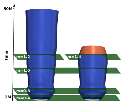
Dynamics of the apparent horizon:
In the computation described above, as can be seen in in the left panel of Fig. 13, the apparent horizon is always present on the computational domain. The horizon mass initially rapidly grows to a value around where it remains roughly constant. Throughout we see that when the regauge safety-net is triggered a slight oscillation in the horizon mass follows. On the other hand when we change grid we see that the horizon mass exhibits a more prominent kink. In the right-hand panel of Fig. 13 we plot the apparent horizons obtained when, less-wisely, the parameter is chosen in the last “Go-to” at . With this choice the apparent horizon rapidly contracts, although the code fails before it leaves the domain. The safety-net is called ever-more frequently as the method insists on forcing the inner boundary to remain pure outflow, until eventually the code crashes at . The physical interpretation of this is that the excision boundary is falling off of the domain, which starts to drift outside the blackhole region, and that the safety-net then forces the worldline of the excision boundary to be spacelike. This interpretation would be clearer if we had an event horizon finder, but is given credence by performing evolutions of a Schwarzschild blackhole with the gauge parameter similarly poorly chosen. In such tests we see that the areal radius of the excision boundary can indeed fall outside of the event horizon at .
IX Conclusions
We have developed a pseudospectral numerical relativity code, bamps, and in so doing have made a series of improvements and investigations into the approach employed in the SpEC code. We presented a set of experiments carefully performed so that direct comparison with either published work, or independent computations of the BAM finite differencing code could be made. These included evolutions of gauge waves, convergence tests, the use of different constraint damping and GHG formulation parameters, scaling tests, perturbed blackhole evolutions and the treatment of supercritical gravitational waves. Ultimately we conclude that the bamps code is working efficiently, scales as desired up to large numbers of processors, and works on sufficiently general grid setups to evolve initial data of interest. Particularly surprising to us was the sensitivity of the method to our modifications of the GHG boundary conditions, even within the class of constraint preserving conditions. This was the case even in our simple evolutions of the Schwarzschild spacetime, so it would be very interesting to see the extent to which such results carry over to compact binary evolutions, be it in SpEC, or in the more distant future in bamps. From the physics point of view, however, our focus is presently on the collapse of axisymmetric gravitational waves. Much of the development reflects this fact. Most notably the implementation of octant symmetry with the Cartoon method gives orders of magnitude speedups over evolving the same data in full 3d. For a recent complimentary approach see SchRin14 . We have additionally written a bespoke axisymmetric apparent horizon finder, which already proved a valuable diagnostic tool, crucial in the evolution of supercritical data, where the existence of an apparent horizon was used as the criterion for moving to an excision grid.
Naturally further developments to the code may be desirable. For physical interpretation, an event horizon finder would complement our apparent horizon finder. A control system like that of SpEC HemSchKid13 would be useful in controlling the positions of the apparent horizons. But the highest priority will likely be in generalizing available grid setups to enable dynamical mesh-refinement.
We have also considered various different types of axisymmetric moment of time-symmetry gravitational wave initial data. In forthcoming work we use bamps to evolve this initial data, close to the critical amplitude separating dispersion and collapse to a blackhole.
Acknowledgements.
We are grateful to Sebastiano Bernuzzi, David Garfinkle, Enno Harms, Sascha Husa, Nathan Kieran Johnson-McDaniel, Harald Pfeiffer and Hannes Rüter for interesting discussions. DH would like to express special gratitude to Helmut Friedrich for interesting discussions and for his warm encouragement. This work was supported in part by the Deutsche Forschungsgemeinschaft (DFG) through its Transregional Center SFB/TR7 “Gravitational Wave Astronomy”, by the DFG Research Training Group 1523/1 “Quantum and Gravitational Fields”, and the Graduierten-Akademie Jena. Computations were performed primarily at the LRZ (Munich).References
- (1) M. W. Choptuik. Consistency of finite-difference solutions of einstein’s equations. Phys. Rev. D, 44:3124–3135, 1991.
- (2) Andrew M. Abrahams and Charles R. Evans. Trapping a geon: Black hole formation by an imploding gravitational wave. Phys. Rev. D, 46:R4117–R4121, 1992.
- (3) Evgeny Sorkin. On critical collapse of gravitational waves. Class. Quant. Grav., 28:025011, 2011.
- (4) John G. Baker, Joan Centrella, Dae-Il Choi, Michael Koppitz, and James van Meter. Gravitational wave extraction from an inspiraling configuration of merging black holes. Phys. Rev. Lett., 96:111102, 2006.
- (5) Manuela Campanelli, Carlos O. Lousto, Pedro Marronetti, and Yosef Zlochower. Accurate evolutions of orbiting black-hole binaries without excision. Phys. Rev. Lett., 96:111101, 2006.
- (6) SpEC - Spectral Einstein Code, http://www.black-holes.org/SpEC.html.
- (7) David Hilditch, Thomas W. Baumgarte, Andreas Weyhausen, Tim Dietrich, Bernd Brügmann, Pedro J. Montero, and Ewald Müller. Collapse of nonlinear gravitational waves in moving-puncture coordinates. Phys.Rev., D88(10):103009, 2013.
- (8) Lee Lindblom, Mark A. Scheel, Lawrence E. Kidder, Robert Owen, and Oliver Rinne. A new generalized harmonic evolution system. Class. Quant. Grav., 23:S447–S462, 2006.
- (9) Miguel Alcubierre, S. R. Brandt, B. Brügmann, D. Holz, E. Seidel, R. Takahashi, and J. Thornburg. Symmetry without symmetry: Numerical simulation of axisymmetric systems using Cartesian grids. Int. J. Mod. Phys. D, 10(3):273–289, 2001. gr-qc/9908012.
- (10) Carsten Gundlach, Jose M. Martin-Garcia, G. Calabrese, and I. Hinder. Constraint damping in the Z4 formulation and harmonic gauge. Class. Quantum Grav., 22:3767–3774, 2005.
- (11) Bela Szilagyi, Lee Lindblom, and Mark A. Scheel. Simulations of binary black hole mergers using spectral methods. Phys. Rev., D80:124010, 2009.
- (12) Luisa T. Buchman and Olivier C. A. Sarbach. Towards absorbing outer boundaries in General Relativity. Class. Quant. Grav., 23:6709–6744, 2006.
- (13) Luisa T. Buchman and Olivier C.A. Sarbach. Improved outer boundary conditions for Einstein’s field equations. Class.Quant.Grav., 24:S307–S326, 2007.
- (14) Oliver Rinne, Lee Lindblom, and Mark A. Scheel. Testing outer boundary treatments for the Einstein equations. Class. Quant. Grav., 24:4053–4078, 2007.
- (15) M. Bjørhus. The ode formulation of hyperbolic pdes discretized by the spectral collocation method. SIAM J. Sci. Comput., 16(3):542–557, 1995.
- (16) Oliver Rinne, Luisa T. Buchman, Mark A. Scheel, and Harald P. Pfeiffer. Implementation of higher-order absorbing boundary conditions for the Einstein equations. Class. Quant. Grav., 26:075009, 2009.
- (17) David Hilditch and Ronny Richter. Hyperbolicity of Physical Theories with Application to General Relativity. 2013.
- (18) C. Ronchi, R. Iacono, and P.S. Paolucci. The “cubed sphere”: A new method for the solution of partial differential equations in spherical geometry. Journal of Computational Physics, 124(1):93 – 114, 1996.
- (19) Jonathan Thornburg. A fast apparent-horizon finder for 3-dimensional Cartesian grids in numerical relativity. Class. Quantum Grav., 21(2):743–766, 21 January 2004.
- (20) Jonathan Thornburg. Black hole excision with multiple grid patches. Class. Quantum Grav., 21(15):3665–3691, 7 August 2004.
- (21) Denis Pollney, Christian Reisswig, Erik Schnetter, Nils Dorband, and Peter Diener. High accuracy binary black hole simulations with an extended wave zone. Phys. Rev. D, 83:044045, 2011.
- (22) Burkhard Zink, Erik Schnetter, and Manuel Tiglio. Multi-patch methods in general relativistic astrophysics. 1. Hydrodynamical flows on fixed backgrounds. Phys.Rev., D77:103015, 2008.
- (23) Erik Schnetter, Peter Diener, Nils Dorband, and Manuel Tiglio. A multi-block infrastructure for three-dimensional time-dependent numerical relativity. Class. Quantum Grav., 23:S553–S578, 2006.
- (24) Luis Lehner, Oscar Reula, and Manuel Tiglio. Multi-block simulations in general relativity: high order discretizations, numerical stability and applications. gr-qc/0507004, 2005.
- (25) Richard Baltensperger and Manfred R. Trummer. Spectral differencing with a twist. J. Sci. Comp., 24(5):1465–1487, 2003.
- (26) J. S. Hesthaven. Spectral penalty methods. Appl. Numer. Math., 33:23–41, 2000.
- (27) Jan S. Hesthaven, Sigal Gottlieb, and David Gottlieb. Spectral Methods for Time-Dependent Problems. Cambridge University Press, Cambridge, 2007.
- (28) Nicholas W. Taylor, Lawrence E. Kidder, and Saul A. Teukolsky. Spectral methods for the wave equation in second-order form. Phys.Rev., D82:024037, 2010.
- (29) D. S. Brill. On the positive definite mass of the Bondi-Weber-Wheeler time-symmetric gravitational waves. Ann. Phys. (N. Y.), 7:466–483, 1959.
- (30) Kenneth R. Eppley. Evolution of time-symmetric gravitational waves: Initial data and apparent horizons. Phys. Rev. D, 16(6):1609–1614, 1977.
- (31) Oliver Rinne. Axisymmetric Numerical Relativity. PhD thesis, University of Cambridge, Cambridge, England, 13 September 2005. gr-qc/0601064.
- (32) D. Holz, W. Miller, M. Wakano, and J. Wheeler. In B. Hu and T. Jacobson, editors, Directions in General Relativity: Proceedings of the 1993 International Symposium, Maryland; Papers in honor of Dieter Brill, Cambridge, England, 1993. Cambridge University Press.
- (33) Masaru Shibata. Time symmetric initial conditions of gravitational waves for 3D numerical relativity. Phys. Rev. D, 55:7529–7537, 1997.
- (34) S. A. Teukolsky. Linearized quadrupole waves in general relativity and the motion of test particles. Phys. Rev. D, 26:745–750, 1982.
- (35) O. Rinne. Constrained evolution in axisymmetry and the gravitational collapse of prolate Brill waves. Classical and Quantum Gravity, 25(13):135009, July 2008.
- (36) Thomas W. Baumgarte and Stuart L. Shapiro. Numerical Relativity: Solving Einstein’s Equations on the Computer. Cambridge University Press, Cambridge, 2010.
- (37) Harald P. Pfeiffer, Lawrence E. Kidder, Mark A. Scheel, and Deirdre Shoemaker. Initial data for Einstein’s equations with superposed gravitational waves. Phys. Rev. D, 71:024020, 2005.
- (38) Marcus Ansorg, Bernd Brügmann, and Wolfgang Tichy. A single-domain spectral method for black hole puncture data. Phys. Rev., D70:064011, 2004.
- (39) Gioel Calabrese, Carsten Gundlach, and David Hilditch. Asymptotically null slices in numerical relativity: Mathematical analysis and spherical wave equation tests. Class.Quant.Grav., 23:4829–4846, 2006.
- (40) Miguel Alcubierre, S. R. Brandt, B. Brügmann, C. Gundlach, Joan Massó, E. Seidel, and P. Walker. Test-beds and applications for apparent horizon finders in numerical relativity. Class. Quantum Grav., 17:2159–2190, 2000.
- (41) Jonathan Thornburg. Event and apparent horizon finders for numerical relativity. Living Rev. Relativity, 2006. [Online article].
- (42) Miguel Alcubierre. Introduction to 3+1 Numerical Relativity. Oxford University Press, Oxford, 2008.
- (43) H.P. de Oliveira and E.L. Rodrigues. Brill wave initial data: Using the Galerkin-collocation method. Phys.Rev., D86:064007, 2012.
- (44) GSL: the GNU Scientific Library: http://www.gnu.org software/gsl/.
- (45) Tim Dietrich and Bernd Brügmann. Solving the Hamiltonian constraint for 1+log trumpets. Phys.Rev., D89:024014, 2014.
- (46) T. W. Baumgarte and S. L. Shapiro. On the Numerical integration of Einstein’s field equations. Phys. Rev., D59:024007, 1998.
- (47) M. Shibata and T. Nakamura. Evolution of three-dimensional gravitational waves: Harmonic slicing case. Phys. Rev., D52:5428–5444, 1995.
- (48) Takashi Nakamura, Ken-ichi Oohara, and Yasufumi Kojima. General relativistic collapse to black holes and gravitational waves from black holes. Prog. Theor. Phys. Suppl., 90:1–218, 1987.
- (49) Frans Pretorius. Numerical relativity using a generalized harmonic decomposition. Class. Quant. Grav., 22:425–451, 2005.
- (50) Andreas Weyhausen, Sebastiano Bernuzzi, and David Hilditch. Constraint damping for the Z4c formulation of general relativity. Phys. Rev. D, 85:024038, 2012.
- (51) Bernd Brügmann, José A. González, Mark Hannam, Sascha Husa, Ulrich Sperhake, and Wolfgang Tichy. Calibration of Moving Puncture Simulations. Phys. Rev. D, 77:024027, 2008.
- (52) David Hilditch, Sebastiano Bernuzzi, Marcus Thierfelder, Zhoujian Cao, Wolfgang Tichy, and Bernd Brügmann. Compact binary evolutions with the Z4c formulation. Phys. Rev. D, 88:084057, 2013.
- (53) Bernd Brügmann. A pseudospectral matrix method for time-dependent tensor fields on a spherical shell. J. Comput. Phys., 235:216–240, 2013.
- (54) G. B. Cook. Initial Data for Numerical Relativity. Living Rev. Relativity, 2000-5, 2000. [Online Article] cited on 30 Sep 2004, http://relativity.livingreviews.org/Articles/lrr-2000-5.
- (55) R. A. Matzner, M. F. Huq, and D. Shoemaker. Initial data and coordinates for multiple black hole systems. Phys. Rev. D, 59:024015, 1998. gr-qc/9805023.
- (56) Gregory B. Cook and Mark A. Scheel. Well-behaved harmonic time slices of a charged, rotating, boosted black hole. Phys. Rev. D, 56:4775, 1997.
- (57) S. Chandrasekhar and S. Detweiler. The quasi-normal modes of the Schwarzschild black hole. Proc. R. Soc. Lond. A., 344:441–452, 1975.
- (58) Tony Chu, Harald P. Pfeiffer, and Michael I. Cohen. Horizon dynamics of distorted rotating black holes. Phys.Rev., D83:104018, 2011.
- (59) Lloyd N. Trefethen. Spectral Methods in MATLAB. SIAM, Philadelphia, 2000.
- (60) Curran D. Muhlberger, Fatemeh Hossein Nouri, Matthew D. Duez, Francois Foucart, Lawrence E. Kidder, et al. Magnetic effects on the low-T/—W— instability in differentially rotating neutron stars. 2014.
- (61) Lee Lindblom and Béla Szilágyi. An Improved Gauge Driver for the GH Einstein System. Phys. Rev., D80:084019, 2009.
- (62) Mark Hannam, Sascha Husa, Denis Pollney, Bernd Brügmann, and Niall Ó Murchadha. Geometry and regularity of moving punctures. Phys. Rev. Lett., 99:241102, 2007.
- (63) Daniel A. Hemberger, Mark A. Scheel, Lawrence E. Kidder, Bela Szilagyi, Geoffrey Lovelace, et al. Dynamical Excision Boundaries in Spectral Evolutions of Binary Black Hole Spacetimes. Class.Quant.Grav., 30:115001, 2013.
- (64) Mark A. Scheel, Matthew Giesler, Daniel A. Hemberger, Geoffrey Lovelace, Kevin Kuper, et al. Improved methods for simulating nearly extremal binary black holes. 2014.
- (65) Christian Schell and Oliver Rinne. Spectral approach to axisymmetric evolution of Einstein’s equations. 2014.