Finite-time Lyapunov dimension and hidden attractor of the Rabinovich system

Abstract

The Rabinovich system, describing the process of interaction between waves in plasma, is considered. It is shown that the Rabinovich system can exhibit a hidden attractor in the case of multistability as well as a classical self-excited attractor. The hidden attractor in this system can be localized by analytical-numerical methods based on the continuation and perpetual points. For numerical study of the attractors’ dimension the concept of finite-time Lyapunov dimension is developed. A conjecture on the Lyapunov dimension of self-excited attractors and the notion of exact Lyapunov dimension are discussed. A comparative survey on the computation of the finite-time Lyapunov exponents by different algorithms is presented and an approach for a reliable numerical estimation of the finite-time Lyapunov dimension is suggested. Various estimates of the finite-time Lyapunov dimension for the hidden attractor and hidden transient chaotic set in the case of multistability are given.

I Introduction

One of the main tasks of the investigation of dynamical systems is the study of established (limiting) behavior of the system after transient processes, i.e., the problem of localization and analysis of attractors (limited sets of system’s states, which are reached by the system from close initial data after transient processes) Poincare-1892 ; Lyapunov-1892 ; LeonovR-1987 . While trivial attractors (stable equilibrium points) can be easily found analytically, the search of periodic and chaotic attractors can turn out to be a challenging problem (see, e.g. famous 16th Hilbert problem Hilbert-1901 on the number of coexisting periodic attractors in two dimensional polynomial systems, which was formulated in 1900 and is still unsolved; see also its generalization for multidimensional systems with chaotic attractors LeonovK-2015-AMC ). For numerical localization of an attractor one needs to choose an initial point in the basin of attraction and observe how the trajectory, starting from this initial point, after a transient process visualizes the attractor. Self-excited attractors, even coexisting in the case of multistability PisarchikF-2014 , can be revealed numerically by the integration of trajectories, started in small neighborhoods of unstable equilibria, while hidden attractors have the basins of attraction, which are not connected with equilibria, and are hidden somewhere in the phase space LeonovK-2013-IJBC ; KuznetsovL-2014-IFACWC ; LeonovKM-2015-EPJST ; Kuznetsov-2016 . Remark that in numerical computation of trajectory over a finite-time interval it is difficult to distinguish a sustained chaos from a transient chaos (a transient chaotic set in the phase space, which can nevertheless persist for a long time) GrebogiOY-1983 . Thus, the search and visualization of hidden attractors and transient sets in the phase space are challenging tasks DudkowskiJKKLP-2016 .

In this paper we study hidden attractors and transient chaotic sets in the Rabinovich system. We show that the methods of numerical continuation and perpetual point are helpful for localization and understanding of hidden attractor in the Rabinovich system.

For the study of chaotic sets and dimension of attractors the concept of the Lyapunov dimension KaplanY-1979 was found useful and became widely spread GrassbergerP-1983 ; EckmannR-1985 ; ConstantinFT-1985 ; AbarbanelBST-1993 ; BoichenkoLR-2005 . Since in numerical experiments we can consider only finite time, in this paper we develop the concept of the finite-time Lyapunov dimension Kuznetsov-2016-PLA and an approach for its reliable numerical computation. Various estimates of the finite-time Lyapunov dimension for the Rabinovich hidden attractor in the case of multistability are given.

II The Rabinovich system: interaction between waves in plasma

Consider a system, suggested in 1978 by M. Rabinovich Rabinovich-1978 ; PikovskiRT-1978 ,

$$\dot{x}=hy-\nu_{1}x-yz,$$ (1)

$$\dot{y}=hx-\nu_{2}y+xz,$$

$$\dot{z}=-z+xy,$$

describing the interaction of three resonantly coupled waves, two of which are parametrically excited. Here, the parameter $h$ is proportional to the pumping amplitude and the parameters $\nu_{1,2}$ are normalized dumping decrements.

After the linear transformation (see, e.g., LeonovB-1992 ):

$$\chi:(x,y,z)\to(\nu_{1}\nu_{2}h^{-1}y,\nu_{1}x,\nu_{1}\nu_{2}h^{-1}z)$$ (2)

and time rescaling:

$$t\to\nu_{1}^{-1}t,$$ (3)

we obtain a generalized Lorenz system:

$$\dot{x}=-\sigma(x-y)-ayz,$$ (4)

$$\dot{y}=rx-y-xz,$$

$$\dot{z}=-bz+xy,$$

where

$$\sigma=\nu_{1}^{-1}\nu_{2},\,b=\nu_{1}^{-1},\,a=-\nu_{2}^{2}h^{-2},\,r=\nu_{1}^{-1}\nu_{2}^{-1}h^{2}.$$ (5)

System (4) with $a=0$ coincides with the classical Lorenz system Lorenz-1963 . As it is discussed in LeonovB-1992 , system (4) can also be used to describe the following physical processes: the convective fluid motion inside rotating ellipsoid, the rotation of rigid body in viscous fluid, the gyrostat dynamics, the convection of horizontal layer of fluid making harmonic oscillations, and the model of Kolmogorov’s flow.

Note that since parameters $\nu_{1}$, $\nu_{2}$, $h$ are positive, the parameters $\sigma$, $b$, $r$ are positive and parameter $a$ is negative. From relation (5) we have:

$$\sigma=-ar.$$ (6)

Further, we study system (4) under the assumption (6). If $r<1$, then system (4) has a unique equilibrium ${\bf\rm S_{0}}=(0,0,0)$, which is globally asymptotically Lyapunov stable (global attractor) LeonovB-1992 ; BoichenkoLR-2005 . If $r>1$, then system (4) has three equilibria: ${\bf\rm S_{0}}=(0,0,0)$ and ${\bf\rm S_{\pm}}=(\pm x_{1},\,\pm y_{1},\,z_{1}),$ where

$$x_{1}=\frac{\sigma b\sqrt{\xi}}{\sigma b+a\xi},\quad y_{1}=\sqrt{\xi},\quad z_{1}=\frac{\sigma\xi}{\sigma b+a\xi},$$

and

$$\xi=\frac{\sigma b}{2a^{2}}\left[a(r-2)-\sigma+\sqrt{(\sigma-ar)^{2}+4a\sigma}\right].$$

The stability of equilibria $S_{\pm}$ of system (4) depends on the parameters $r$, $a$, and $b$. Using the Routh-Hurwitz criterion, we obtain the following

Lemma 1.

The equilibria $S_{\pm}$ of system (4) with parameters (5) are stable if and only if one of the following conditions holds:

1. $0\leq\,ar+1\,<\frac{2r}{r-\sqrt{r(r-1)}}$,

2. $ar+1<0$,   $b>b_{\rm cr}=\frac{4a(r-1)(ar+1)\sqrt{r(r-1)}+(ar-1)^{3}}{(ar+1)^{2}-4ar^{2}}.$

Sketch of the proof. The coefficients of the characteristic polynomial $\chi(x,\,y,\,z)=\lambda^{3}+p_{1}(x,\,y,\,z)\lambda^{2}+p_{2}(x,\,y,\,z)\lambda+p_{3}(x,\,y,\,z)$ of the Jacobian matrix of system (4) at the point $(x,\,y,\,z)$ are the following

$$p_{1}(x,\,y,\,z)=b-ar+1,$$

$$p_{2}(x,\,y,\,z)=x^{2}+ay^{2}-az^{2}-ar(b-r+1)+b,$$

$$p_{3}(x,\,y,\,z)=-a\big{(}2xyz+rx^{2}-y^{2}+bz^{2}-br(r-1)\big{)}.$$

One can check that inequalities $p_{1}(x_{1},\,y_{1},\,z_{1})>0$ and $p_{3}(x_{1},\,y_{1},\,z_{1})>0$ are always valid. If $ar+1\geq 0$, then $p_{1}(x_{1},\,y_{1},\,z_{1})p_{2}(x_{1},\,y_{1},\,z_{1})-p_{3}(x_{1},\,y_{1},\,z_{1})>0$, and if condition (i) also holds, then $p_{2}(x_{1},\,y_{1},\,z_{1})>0$.

If $ar+1<0$, then $p_{2}(x_{1},\,y_{1},\,z_{1})>0$, and if condition (ii) also holds, then $p_{1}(x_{1},\,y_{1},\,z_{1})p_{2}(x_{1},\,y_{1},\,z_{1})-p_{3}(x_{1},\,y_{1},\,z_{1})>0$. ∎

III Attractors and transient chaos

Consider system (4) as an autonomous differential equation of a general form:

$$\dot{u}=f({u}),$$ (7)

where $u=(x,y,z)\in\mathbb{R}^{3}$, and the continuously differentiable vector-function $f:\mathbb{R}^{3}\to\mathbb{R}^{3}$ represents the right-hand side of system (4). Define by ${u}(t,{u}_{0})$ a solution of (7) such that ${u}(0,{u}_{0})={u}_{0}$. For system (7), a bounded closed invariant set $K$ is

1. a (local) attractor if it is a minimal locally attractive set (i.e. $\lim_{t\to+\infty}{\rm dist}(K,{u}(t,{u}_{0}))=0$ $\forall{u_{0}}\in K(\varepsilon)$, where $K(\varepsilon)$ is a certain $\varepsilon$-neighborhood of set $K$),

2. a global attractor if it is a minimal globally attractive set (i.e. $\lim_{t\to+\infty}{\rm dist}(K,{u}(t,{u}_{0}))=0$ $\forall{u_{0}}\in\mathbb{R}^{3}$),

where ${\rm dist}(K,{u})=\inf_{{v}\in K}||{v}-{u}||$ is the distance from the point ${u}\in\mathbb{R}^{3}$ to the set $K\subset\mathbb{R}^{3}$ (see, e.g. LeonovKM-2015-EPJST ).

Note that system (4) (or (7)) is dissipative in the sense that it possesses a bounded convex absorbing set LeonovB-1992 ; LeonovKM-2015-EPJST :

$$\mathcal{B}(r,a,b)=\left\{u\in\mathbb{R}^{3}\leavevmode\nobreak\ |\leavevmode\nobreak\ V(u)\leq\frac{b(\sigma+\delta r)^{2}}{2c(a+\delta)}\right\},$$ (8)

where $V(u)=V(x,y,z)=x^{2}+\delta y^{2}+(a+\delta)\left(z-\frac{\sigma+\delta r}{a+\delta}\right)^{2}$, $\delta$ is an arbitrary positive number such that $a+\delta>0$ and $c=\min(\sigma,1,\frac{b}{2})$. Thus, the solutions of (4) exist for $t\in[0,+\infty)$ and system (4) possesses a global attractor Chueshov-2002-book ; LeonovKM-2015-EPJST , which contains the set of all equilibria and can be constructed as $\cap_{\tau>0}\overline{\cup_{t\geq\tau}\varphi^{t}\left(\mathcal{B}\right)}$.

Computational errors (caused by a finite precision arithmetic and numerical integration of differential equations) and sensitivity to initial data allow one to get a reliable visualization of a chaotic attractor by only one pseudo-trajectory computed for a sufficiently large time interval. One needs to choose an initial point in the basin of attraction of the attractor and observe how the trajectory, starting from this initial point, after a transient process visualizes the attractor. Thus, from a computational point of view, it is natural to suggest the following classification of attractors, based on the simplicity of finding the basins of attraction in the phase space.

Definition 1.

LeonovKV-2011-PLA ; LeonovK-2013-IJBC ; LeonovKM-2015-EPJST ; Kuznetsov-2016 An attractor is called a self-excited attractor if its basin of attraction intersects with any open neighborhood of an equilibrium, otherwise, it is called a hidden attractor.

For a self-excited attractor its basin of attraction is connected with an unstable equilibrium and, therefore, self-excited attractors can be localized numerically by the standard computational procedure in which after a transient process a trajectory, starting in a neighborhood of an unstable equilibrium, is attracted to the state of oscillation and then traces it. Thus, self-excited attractors can be easily visualized (e.g. the classical Lorenz, Rössler, and Hénon attractors are self-excited with respect to unstable zero equilibrium and can be easily visualized by a trajectory from its vicinity).

For a hidden attractor, its basin of attraction is not connected with equilibria and, thus, the search and visualization of hidden attractors in the phase space may be a challenging task. Hidden attractors are attractors in the systems without equilibria (see, e.g. rotating electromechanical systems with Sommerfeld effect (1902) Sommerfeld-1902 ; KiselevaKL-2016-IFAC ), and in the systems with only one stable equilibrium (see, e.g. counterexamples LeonovK-2011-DAN ; LeonovK-2013-IJBC to Aizerman’s (1949) and Kalman’s (1957) conjectures on the monostability of nonlinear control systems Aizerman-1949 ; Kalman-1957 ). One of the first related problems is the second part of 16th Hilbert problem Hilbert-1901 on the number and mutual disposition of limit cycles in two dimensional polynomial systems, where nested limit cycles (a special case of multistability and coexistence of periodic attractors) exhibit hidden periodic attractors (see, e.g., Bautin-1939 ; KuznetsovKL-2013-DEDS ; LeonovK-2013-IJBC ). The classification of attractors as being hidden or self-excited was introduced by Leonov & Kuznetsov in connection with the discovery of the first hidden Chua attractor KuznetsovLV-2010-IFAC ; LeonovKV-2011-PLA ; BraginVKL-2011 ; LeonovKV-2012-PhysD ; KuznetsovKLV-2013 ; KiselevaKKKLYY-2017 ; StankevichKLC-2017 and has captured much attention of scientists from around the world (see, e.g. BurkinK-2014-HA ; LiSprott-2014-HA ; LiZY-2014-HA ; PhamRFF-2014-HA ; ChenLYBXW-2015-HA ; KuznetsovKMS-2015-HA ; SahaSRC-2015-HA ; SemenovKASVA-2015 ; SharmaSPKL-2015-EPJST ; ZhusubaliyevMCM-2015-HA ; DancaKC-2016 ; JafariPGMK-2016-HA ; MenacerLC-2016-HA ; OjoniyiA-2016-HA ; PhamVJVK-2016-HA ; RochaM-2016-HA ; WeiPKW-2016-HA ; Zelinka-2016-HA ; BorahR-2017-HA ; BrzeskiWKKP-2017 ; FengP-2017-HA ; JiangLWZ-2016-HA ; KuznetsovLYY-2017-CNSNS ; MaWJZH-2017 ; MessiasR-2017-HA ; SinghR-2017-HA ; VolosPZMV-2017-HA ; WeiMSAZ-2017-HA ; ZhangWWM-2017-HA ).

Since in the numerical computation of trajectory over a finite-time interval it is difficult to distinguish a sustained chaos from a transient chaos (a transient chaotic set in the phase space, which can nevertheless persist for a long time) GrebogiOY-1983 ; LaiT-2011 , a similar to the above classification can be introduced for the transient chaotic sets.

Definition 2.

DancaK-2017-CSF ; ChenKLM-2017-IJBC A transient chaotic set is called a hidden transient chaotic set if it does not involve and attract trajectories from a small neighborhood of equilibria; otherwise, it is called self-excited.

In order to distinguish an attracting chaotic set (attractor) from a transient chaotic set in numerical experiments, one can consider a grid of points in a small neighborhood of the set and check the attraction of corresponding trajectories towards the set.

For system (1) with parameters $\nu_{1}=1$, $\nu_{2}=4$, and increasing $h$ it is possible to observe PikovskiRT-1978 the classical scenario of transition to chaos (via homoclinic and subcritical Andronov-Hopf bifurcations) similar to the scenario in the Lorenz system. For $4.84\lessapprox h\lessapprox 13.4$ in system (1) there is a self-excited chaotic attractor (see e.g. Fig. 1), which coexists with two stable equilibria. The same scenario can be obtained for system (4) when parameters $b>0$ and $a<0$ are fixed and $r$ is increasing. Besides self-excited chaotic attractors, a hidden attractor was found in the system KuznetsovLMS-2016-INCAAM ; ChenKLM-2017-IJBC . Note that in LeonovKM-2015-CNSNS ; LeonovKM-2015-EPJST system (4) with $a>0$ was studied and a hidden attractor was also found numerically.

In this work we localize a hidden chaotic attractor in system (4) with $a<0$ by the numerical continuation method starting from a self-excited chaotic attractor. We change parameters, considered in KuznetsovLMS-2016-INCAAM , in such a way that the chaotic set locates not too close to the unstable zero equilibrium to avoid a situation, when numerically integrated trajectory oscillates for a long time and then falls on the unstable manifold of unstable zero equilibrium, leaves the chaotic set, and tends to one of the stable equilibria.

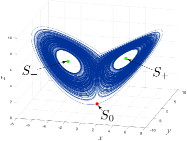
Figure 1: Multistability in the Rabinovich system (4) with the classical values of parameters $\nu_{1}=1$, $\nu_{2}=4$, $h=4.92$ from PikovskiRT-1978 : coexistence of three local attractors — two stable equilibria $S_{\pm}$ and a chaotic self-excited attractor (self-excited with respect to the unstable zero equilibrium $S_{0}$).

III.1 Localization via numerical continuation method

One of the effective methods for numerical localization of hidden attractors in multidimensional dynamical systems is based on the homotopy and numerical continuation method (NCM). The idea is to construct a sequence of similar systems such that for the first (starting) system the initial point for numerical computation of oscillating solution (starting attractor) can be obtained analytically, e.g, it is often possible to consider the starting system with a self-excited starting attractor; then the transformation of this starting attractor in the phase space is tracked numerically while passing from one system to another; the last system corresponds to the system in which a hidden attractor is searched.

For the study of the scenario of transition to chaos, we consider system (7) with $f(u)=f(u,\lambda)$, where $\lambda\in\Lambda\subset\mathbb{R}^{d}$ is a vector of parameters whose variation in the parameter space $\Lambda$ determines the scenario. Let $\lambda_{\rm end}\in\Lambda$ define a point corresponding to the system, where a hidden attractor is searched. Choose a point $\lambda_{\rm begin}\in\Lambda$ such that we can analytically or numerically localize a certain nontrivial (oscillating) attractor $\mathcal{A}^{1}$ in system (7) with $\lambda=\lambda_{\rm begin}$ (e.g., one can consider an initial self-excited attractor, defined by a trajectory ${u}^{1}(t)$ numerically integrated on a sufficiently large time interval $t\in[0,T]$ with the initial point ${u}^{1}(0)$ in the vicinity of an unstable equilibrium). Consider a path in the parameter space $\Lambda$ , i.e. a continuous function $\gamma\leavevmode\nobreak\ :\leavevmode\nobreak\ [0,\,1]\to\Lambda$, for which $\gamma(0)=\lambda_{\rm begin}$ and $\gamma(1)=\lambda_{\rm end}$, and a sequence of points $\{\lambda^{j}\}_{j=1}^{k}$ on the path, where $\lambda^{1}=\lambda_{\rm begin}$, $\lambda^{k}=\lambda_{\rm end}$, such that the distance between $\lambda^{j}$ and $\lambda^{j+1}$ is sufficiently small. On each next step of the procedure, the initial point for a trajectory to be integrated is chosen as the last point of the trajectory integrated on the previous step: ${u}^{j+1}(0)={u}^{j}(T)$. Following this procedure and sequentially increasing $j$, two alternatives are possible: the points of $\mathcal{A}^{j}$ are in the basin of attraction of attractor $\mathcal{A}^{j+1}$ or, while passing from system (7) with $\lambda=\lambda^{j}$ to system (7) with $\lambda=\lambda^{j+1}$, a loss of stability bifurcation is observed and attractor $\mathcal{A}^{j}$ vanishes. If while changing $\lambda$ from $\lambda_{\rm begin}$ to $\lambda_{\rm end}$ there is no loss of stability bifurcation of the considered attractors, then a hidden attractor for $\lambda^{k}=\lambda_{\rm end}$ (at the end of the procedure) is localized.

III.2 Localization using perpetual points

The equilibrium points of a dynamical system are the ones, where the velocity and acceleration of the system simultaneously become zero. If the existing equilibrium points are unstable, then we may get either oscillating or unbounded solutions. In this section we show numerical results, which suggest that there are points, termed as perpetual points Prasad-2015 , which may help to visualize hidden attractors.

For system (7), the equilibrium points ${u}_{\rm ep}$ are defined by the equation $\dot{u}=f({u}_{\rm ep})=0$. Consider a derivative of system (7) with respect to time

$$\ddot{u}=J({u})\,f({u})=g({u}),$$ (9)

where $J(u)=\left[\frac{\partial f_{i}(u)}{\partial u_{j}}\right]_{i,j=1}^{n}$ is the $n\times n$ Jacobian matrix. Here $g({u})$ may be termed as an acceleration vector. System (9) shows the variation of acceleration in the phase space.

Similar to the equilibrium points estimation, where we set the velocity vector to zero, we can also get a set of points, where $\ddot{u}=g({u}_{\rm pp})=0$ in (9), i.e. the points corresponding to the zero acceleration. At these points the velocity $\dot{u}$ may be either zero or nonzero. This set includes the equilibrium points ${u}_{\rm ep}$ with zero velocity as well as a subset of points with nonzero velocity. These nonzero velocity points ${u}_{\rm pp}$ are termed as perpetual points Prasad-2015 ; DudkowskiPK-2015-HA ; Prasad-2016 ; DudkowskiJKKLP-2016 . The reason why perpetual points may lead to hidden states (perpetual point method (PPM)) is still not well understood (see, e.g. discussion in NazarimehrSJS-2017 ).

Lemma 2.

Perpetual points $S_{\rm pp}=(x_{\rm pp},y_{\rm pp},z_{\rm pp})$ of system (4) can be derived from the following system

$$\left\{\begin{aligned} &(x_{\rm pp}^{2}-az_{\rm pp}^{2}+ar^{2}-1)\left(-y_{\rm pp}^{2}+z_{\rm pp}^{2}+r^{2}(a-1)\right)=\\ &\qquad\qquad\qquad\quad=r^{2}(ar-1)^{2}-z_{\rm pp}^{2}(ar-b-1)^{2},\\ &2x_{\rm pp}y_{\rm pp}z_{\rm pp}+rx_{\rm pp}^{2}-y_{\rm pp}^{2}+bz_{\rm pp}^{2}-br(r-1)=0,\\ &z_{\rm pp}=\frac{rx_{\rm pp}^{2}+(ar-b-1)x_{\rm pp}y_{\rm pp}-ary_{\rm pp}^{2}}{x_{\rm pp}^{2}+ay_{\rm pp}^{2}-b^{2}}.\end{aligned}\right.$$ (10)

IV Hidden attractor in
the Rabinovich system

Next we apply the NCM for localization of a hidden attractor in the Rabinovich system (4) and check whether the attractor can be also localized using PPM.

In this experiment, we fix parameter $r$ and, using condition (ii) of Lemma 1, define parameters $a=-\frac{1}{r}-\varepsilon_{1}$ and $b=b_{\rm cr}-\varepsilon_{2}$. For $r=100$, $\varepsilon_{1}=10^{-3}$, $\varepsilon_{2}=10^{-2}$ we obtain $a=a_{0}\equiv-1.1\cdot 10^{-2}$, $b=b_{0}\equiv 6.7454\cdot 10^{-2}$ and take $P_{0}(a_{0},\,b_{0})$ as the initial point of line segment on the plane $(a,\,b)$. The eigenvalues of the Jacobian matrix at the equilibria $S_{0}$, $S_{\pm}$ of system (4) for these parameters are the following:

$$S_{0}\, :\quad 9.4382,\quad-0.0675,\quad-11.5382,$$

$$S_{\pm}\, :\quad 0.0037\pm 3.6756\,\mathrm{i},\quad-2.1749.$$

Consider on the plane $(a,\,b)$ a line segment, intersecting a boundary of stability domain of the equilibria $S_{\pm}$, with the final point $P_{2}(a_{2},\,b_{2})$, where $a_{2}=a_{0}+1.035\leavevmode\nobreak\ \cdot\leavevmode\nobreak\ 10^{-3}=-9.965\cdot 10^{-3}$, $b_{2}=b_{0}+\varepsilon_{2}=7.7454\cdot 10^{-2}$, i.e. the equilibrium $S_{0}$ remains saddle and the equilibria $S_{\pm}$ become stable focus-nodes

$$S_{0}\, :\quad 8.9842,\quad-0.0775,\quad-10.9807,$$

$$S_{\pm}\, :\quad-0.0401\pm 3.9152\,\mathrm{i},\quad-1.9937.$$

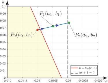
Figure 2: Path $P_{0}(a_{0},\,b_{0})\to P_{1}(a_{1},\,b_{1})\to P_{2}(a_{2},\,b_{2})$ in parameters plane $(a,\,b)$ for the localization of hidden attractor in system (4) with $r=100$. Here $a_{0}=-1.1\cdot 10^{-2}$, $b_{0}=6.7454\cdot 10^{-2}$, $a_{1}=-1.049\cdot 10^{-2}$, $b_{1}=7.2454\cdot 10^{-2}$, $a_{2}=-9.965\cdot 10^{-3}$, $b_{2}=7.7454\cdot 10^{-3}$; $(\bullet)$ $P_{0}(a_{0},\,b_{0})$: self-excited attractor with respect to $S_{0}$, $S_{\pm}$; $(\bullet)$ $P_{1}(a_{1},\,b_{1})$: self-excited attractor with respect to $S_{0}$; $(\bullet)$ $P_{2}(a_{2},\,b_{2})$: hidden attractor. Stability domain is defined using Lemma 1.

The initial point $P_{0}(a_{0},\,b_{0})$ corresponds to parameters for which in system (4) there exists a self-excited attractor. Then for the considered line segment a sufficiently small partition step is chosen and at each iteration step of the procedure an attractor in the phase space of system (4) is computed. The last computed point at each step is used as the initial point for the computation at the next step. In this experiment we use NCM with $3$ steps on the path $P_{0}(a_{0},\,b_{0})\to P_{1}(a_{1},\,b_{1})\to P_{2}(a_{2},\,b_{2})$, with $a_{1}=\frac{1}{2}(a_{0}+a_{2})$, $b_{1}=\frac{1}{2}(b_{0}+b_{2})$ (see Fig. 2). At the first step we have self-excited attractor with respect to unstable equilibria $S_{0}$ and $S_{\pm}$; at the second step the equilibria $S_{\pm}$ become stable but the attractor remains self-excited with respect to equilibrium $S_{0}$; at the third step it is possible to visualize a hidden attractor of system (4) (see Fig. 3).

Using Lemma 2 for parameters $r=100$, $a=-9.965\cdot 10^{-3}$, $b=7.7454\cdot 10^{-2}$, we obtain one perpetual point $S_{\rm pp}=(-0.2385,49.1403,-101.4613)$, which allows one to localize a hidden attractor (see Fig. 4). Hence, here both NCM and PPM allow one to find this hidden attractor.

Around equilibrium $S_{0}$ we choose a small spherical vicinity of radius $\delta$ (in our experiments we check $\delta\in[0.1,0.5]$) and take $N$ random initial points on it (in our experiment $N=4000$). Using MATLAB, we integrate system (4) with these initial points in order to explore the obtained trajectories. We repeat this procedure several times in order to get different initial points for trajectories on the sphere. We get the following results: all the obtained trajectories either attract to the stable equilibrium $S_{+}$ or the equilibrium $S_{-}$ and do not tend to the attractor. This gives us a reason to classify the chaotic attractor, obtained in system (4), as the hidden one.

Remark that there exist hidden chaotic sets in the Rabinovich system, which cannot be localized by PPM. For example, for parameters $r=6.8$, $a=-0.5$, $b\in[0.99,\,1]$ KuznetsovLMS-2016-INCAAM , the hidden attractor obtained by NCM is not localizable via PPM (see Fig. 5).

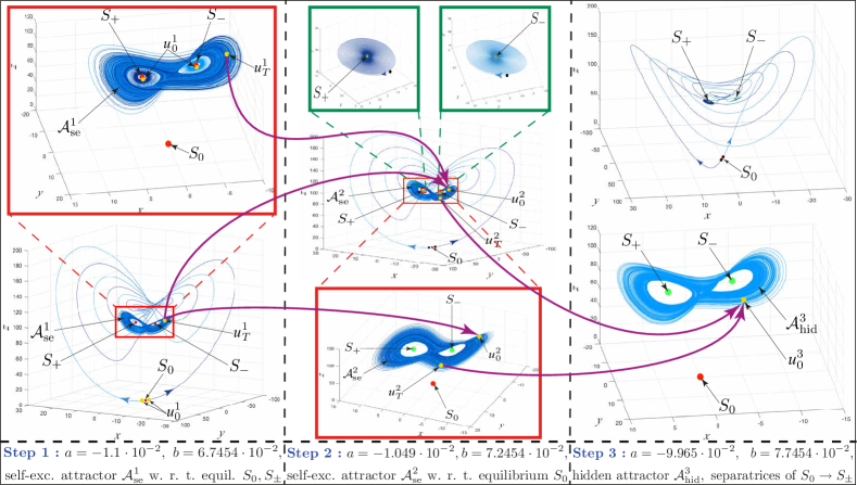
Figure 3: Localization, by NCM, of a hidden attractor in system (4) with $r=100$, $a=-9.965\cdot 10^{-3}$, $b=7.7454\cdot 10^{-2}$. Trajectories $u^{i}(t)=(x^{i}(t),y^{i}(t),z^{i}(t)$ (blue) are defined on the time interval $[0,T]$, $T=10^{3}$ and initial point (yellow) on $(i+1)$-th iteration is defined as $u_{0}^{i+1}:=u_{T}^{i}$ (violet arrows), where $u_{T}^{i}=u^{i}(T)$ is a final point (yellow).

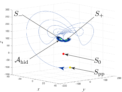
Figure 4: Localization of hidden attractor in system (4) with $r=100$, $a=-9.965\cdot 10^{-3}$, $b=7.7454\cdot 10^{-2}$ from the perpetual point $S_{\rm pp}=(-0.2385,49.1403,-101.4613)$.

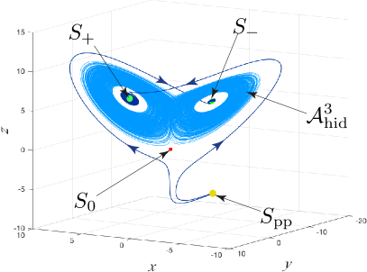
Figure 5: Hidden attractor in system (4) with $r=6.8$, $a=-0.5$, $b=0.99$ which can be localized via NCM (initial point ${u}_{0}=(-0.1629,\,-0.2154,\,1.9553)$), but cannot be localized from the perpetual point $S_{\rm pp}=(0.7431,-12.6109,-7.4424)$ (yellow).

V Computation of the Lyapunov dimension

V.1 The Lyapunov dimension and Lyapunov exponents: finite-time and limit values.

For the study of attractors the Lyapunov exponents Lyapunov-1892 and Lyapunov dimension KaplanY-1979 are found useful and have become widely spread (see, e.g. GrassbergerP-1983 ; EckmannR-1985 ; ConstantinFT-1985 ; AbarbanelBST-1993 ; BoichenkoLR-2005 ). Since in numerical experiments we can consider only finite time, in this paper we develop the concept of the finite-time Lyapunov dimension Kuznetsov-2016-PLA and an approach to its reliable numerical computation.

Nowadays, various approaches to the Lyapunov dimension definition are used. Here, we follow the definition of finite-time Lyapunov dimension from Kuznetsov-2016-PLA inspirited by the works of Douady & Oesterlé DouadyO-1980 , Hunt Hunt-1996 , and Rabinovich et al. RabinovichEW-2000 .

Define by $u(t,u_{0})$ a solution of system (7) such that $u(0,u_{0})=u_{0}$, and consider a map given by the evolutionary operator $\varphi^{t}(u_{0})=u(t,u_{0})$ (shift operator along a solution of (7)). Since system (7) poses an absorbing set (see (8)), the uniqueness and existence of solutions of system (7) for $t\in[0,+\infty)$ take place and the system generates a dynamical system $\{\varphi^{t}\}_{t\geq 0}$. Let a nonempty closed bounded set $K\subset\mathbb{R}^{3}$ be invariant with respect to dynamical system generated by (7) $\{\varphi^{t}\}_{t\geq 0}$, i.e. $\varphi^{t}(K)=K$ for all $t\geq 0$ (e.g. $K$ is an attractor). Further we use compact notations for finite-time local Lyapunov dimension: $\dim_{\rm L}(t,u)=\dim_{\rm L}(\varphi^{t},u)$, the finite-time Lyapunov dimension: $\dim_{\rm L}(t,K)=\dim_{\rm L}(\varphi^{t},K)$, and for the Lyapunov dimension (or the Lyapunov dimension of dynamical system $\{\varphi^{t}\}_{t\geq 0}$ with respect to $K$): $\dim_{\rm L}K=\dim_{\rm L}(\{\varphi^{t}\}_{t\geq 0},K)$.

Consider linearization of system (7) along the solution $\varphi^{t}(u)$:

$$\dot{v}=J(\varphi^{t}(u))v,\quad J(u)=Df(u),$$ (11)

where $J(u)$ is the $3\!\times\!3$ Jacobian matrix, the elements of which are continuous functions of $u$. Suppose that $\det J(u)\neq 0\quad\forall u\in\mathbb{R}^{3}$. Consider a fundamental matrix of solutions of linear system (11), $D\varphi^{t}(u)$, such that $D\varphi^{0}(u)=I$, where $I$ is a unit $3\!\times\!3$ matrix. Let $\sigma_{i}(t,u)=\sigma_{i}(D\varphi^{t}(u))$, $i=1,2,3$, be the singular values of $D\varphi^{t}(u)$ (i.e. $\sigma_{i}(t,u)>0$ and ${\sigma_{i}(t,u)}^{2}$ are the eigenvalues of the symmetric matrix $D\varphi^{t}(u)^{*}D\varphi^{t}(u)$ with respect to their algebraic multiplicity), ordered so that $\sigma_{1}(t,u)\geq\sigma_{2}(t,u)\geq\sigma_{3}(t,u)>0$ for any $u$ and $t$. A singular value function of order $d\in[0,3]$ is defined as

$$\omega_{d}(D\varphi^{t}(u))=\sigma_{1}(t,u)\cdots\sigma_{\lfloor d\rfloor}(t,u)\sigma_{\lfloor d\rfloor+1}(t,u)^{d-\lfloor d\rfloor},$$

$$\omega_{0}(D\varphi^{t}(u))=1,\omega_{3}(D\varphi^{t}(u))=\sigma_{1}(t,u)\sigma_{2}(t,u)\sigma_{3}(t,u),$$

where ${\lfloor d\rfloor}$ is the largest integer less or equal to $d$. For a certain moment of time $t$ finite-time local Lyapunov dimension at the point $u$ is defined as Kuznetsov-2016-PLA

$$\dim_{\rm L}(t,u)=\max\{d\in[0,3]:\omega_{d}(D\varphi^{t}(u))\geq 1\}$$ (12)

and the finite-time Lyapunov dimension of $K$ is defined as

$$\dim_{\rm L}(t,K)=\sup\limits_{u\in K}\dim_{\rm L}(t,u).$$ (13)

The Douady–Oesterlé theorem DouadyO-1980 implies that for any fixed $t>0$ the Lyapunov dimension of the map $\varphi^{t}$ with respect to a closed bounded invariant set $K$, defined by (13), is an upper estimate of the Hausdorff dimension of the set $K$: $\dim_{\rm H}K\leq\dim_{\rm L}(t,K)$.

For the estimation of the Hausdorff dimension of invariant closed bounded set $K$ one can use the map $\varphi^{t}$ with any time $t$ (e.g. $t=0$ leads to the trivial estimate $\dim_{\rm H}K\leq 3$) and, thus, the best estimation is $\dim_{\rm H}{K}\leq\inf_{t\geq 0}\dim_{\rm L}(t,K).$ The following property

$$\inf_{t\geq 0}\sup\limits_{u\in K}\dim_{\rm L}(t,u)=\liminf_{t\to+\infty}\sup\limits_{u\in K}\dim_{\rm L}(t,u)$$ (14)

allows one to introduce the Lyapunov dimension of $K$ as Kuznetsov-2016-PLA

$$\dim_{\rm L}K=\liminf_{t\to+\infty}\sup\limits_{u\in K}\dim_{\rm L}(t,u)$$ (15)

and get an upper estimation of the Hausdorff dimension:

$$\dim_{\rm H}{K}\leq\dim_{\rm L}K.$$

Recall that a set with noninteger Hausdorff dimension is referred to as a fractal set EckmannR-1985 .

Consider a set of finite-time Lyapunov exponents at the point $u$:

$$\operatorname{LE}_{i}(t,u)=\frac{1}{t}\ln\sigma_{i}(t,u),\ t>0,\quad i=1,2,3.$$ (16)

Here the set $\{\operatorname{LE}_{i}(t,u)\}_{i=1}^{3}$ is ordered by decreasing (i.e. $\operatorname{LE}_{1}(t,u)\geq\operatorname{LE}_{2}(t,u)\geq\operatorname{LE}_{3}(t,u)$ for all $t>0$). Then for $j(t,u)=\lfloor\dim_{\rm L}(t,u)\rfloor<3$ and $s(t,u)=\dim_{\rm L}(t,u)-\lfloor\dim_{\rm L}(t,u)\rfloor$ we have $0=\frac{1}{t}\ln(\omega_{j(t,u)+s(t,u)}(D\varphi^{t}(u)))=\sum_{i=1}^{j(t,u)}\operatorname{LE}_{i}(t,u)+s(t,u)\operatorname{LE}_{j(t,u)+1}(t,u)$ and $j(t,u)=\max\{m:\sum_{i=1}^{m}\operatorname{LE}_{i}(t,u)\geq 0\}$. Thus, we get an analog of the Kaplan-Yorke formula KaplanY-1979 with respect to the set of finite-time Lyapunov exponents $\{\operatorname{LE}_{i}(t,u)\}_{i=1}^{3}$ Kuznetsov-2016-PLA :

$$\!\!\!d_{\rm L}^{\rm KY}\!(\!\{\!\operatorname{LE}_{i}(t,\!u)\!\}_{i=1}^{3}\!)\!=\!j(t,u)+\tfrac{\operatorname{LE}_{1}(t,u)+\cdot\cdot+\operatorname{LE}_{j(t,u)}(t,u)}{|\operatorname{LE}_{j(t,u)\!+\!1}(t,u)|}$$ (17)

which gives the finite-time local Lyapunov dimension:

$$\dim_{\rm L}(t,u)=d_{\rm L}^{\rm KY}(\{\operatorname{LE}_{i}(t,u)\}_{i=1}^{3}).$$

Thus, in the above approach the use of Kaplan-Yorke formula (17) with the finite-time Lyapunov exponents $\{\operatorname{LE}_{i}(t,u)\}_{i=1}^{3}$ is rigorously justified by the Douady–Oesterlé theorem.

Note that the finite-time local Lyapunov dimension is invariant under time scaling: $t\to at,a>0$ (e.g., it follows from (16) and (17)), and the Lyapunov dimension is invariant under Lipschitz diffeomorphisms KuznetsovAL-2016 ; Kuznetsov-2016-PLA , i.e. if the dynamical system $\{\varphi^{t}\}_{t\geq 0}$ and its closed bounded invariant set $K$ under a smooth change of coordinates $w=\chi(u)$ are transformed to the dynamical system $\{\varphi_{\chi}^{t}\}_{t\geq 0}$ and its closed bounded invariant set $\chi(K)$, respectively, then $\dim_{\rm L}(\{\varphi^{t}\}_{t\geq 0},K)=\dim_{\rm L}(\{\varphi_{\chi}^{t}\}_{t\geq 0},\chi(K)).$

V.2 Algorithm for numerical computation
of the finite-time Lyapunov dimension

Applying the statistical physics approach and assuming the ergodicity (see, e.g. KaplanY-1979 ; Ledrappier-1981 ; FredericksonKYY-1983 ; FarmerOY-1983 ), the Lyapunov dimension of attractor $\dim_{\rm L}K$ is often estimated by the local Lyapunov dimension $\dim_{\rm L}(t,u_{0})$, corresponding to a “typical” trajectory, which belongs to the attractor: $\{u(t,u_{0}),t\geq 0\},\ u_{0}\in K$, and its limit value $\lim_{t\to+\infty}\dim_{\rm L}(t,u_{0})$. However, from a practical point of view, the rigorous proof of ergodicity is a challenging task BogoliubovK-1937 ; DellnitzJ-2002 ; Oseledec-1968 ; Ledrappier-1981 and hardly it can effectively be done in a general case (see, e.g. discussions in BarreiraS-2000 (ChaosBook, , p.118)OttY-2008 (Young-2013, , p.9) (PikovskyP-2016, , p.19), and the works KuznetsovL-2005 ; LeonovK-2007 on the Perron effects of the largest Lyapunov exponent sign reversals). An example of the rigorous use of the ergodic theory for effective estimation of the Lyapunov dimensions can be found, e.g. in Schmeling-1998 . In one of the pioneering works by Yorke et al. (FredericksonKYY-1983, , p.190) the exact limit values of finite-time Lyapunov exponents $\{\lim\limits_{t\to+\infty}\operatorname{LE}_{i}(t,u)\}_{i}^{3}=\{\operatorname{LE}_{i}(u)\}$, if they exist and are the same for all $u\in K$ $\big{(}$i.e. $\{\operatorname{LE}_{i}(u)\}_{i}^{3}\equiv\{\operatorname{LE}_{i}\}_{i}^{3}$ $\forall u\in K$ and $\dim_{\rm L}K=d_{\rm L}^{\rm KY}(\{\operatorname{LE}_{i}\}_{1}^{3})=j+\tfrac{\operatorname{LE}_{1}+\cdots+\operatorname{LE}_{j}}{|\operatorname{LE}_{j+1}|}$$\big{)}$, are called the absolute ones, and it is noted that the absolute Lyapunov exponents rarely exist. Note also that even if a numerical approximation (visualization) $\widetilde{K}$ of the attractor $K$ is obtained, it is not straightforward how to get a point on the attractor itself: $u\in K$.

Thus, a rather easy way to get reliable estimation of the Lyapunov dimension of attractor $K$ is to localize the attractor $K\subset K^{\varepsilon}$, to consider a grid of points $K^{\varepsilon}_{\rm grid}$ on $K^{\varepsilon}$, and to find the maximum of the corresponding finite-time local Lyapunov dimensions for a certain time $t=T$: $\max\limits_{u\in K^{\varepsilon}_{\rm grid}}\dim_{\rm L}(\varphi^{T},u)=\max\limits_{u\in K^{\varepsilon}_{\rm grid}}j(T,u)+\frac{\operatorname{LE}_{1}(T,u)+\cdots+\operatorname{LE}_{j(T,u)}(T,u)}{|\operatorname{LE}_{j(T,u)+1}(T,u)|}$.

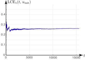
(a) $\operatorname{LCE}_{1}(t,\,u_{\rm init})$, $t\in[0,\leavevmode\nobreak\ T_{1}]$,   $T_{1}\approx 15295$.

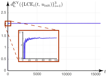
(b) ${d}_{\rm L}^{\rm KY}(\{\operatorname{LCE}_{i}(t,\,u_{\rm init})\}_{i=1}^{3})$, $t\in[0,\leavevmode\nobreak\ T_{1}]$,   $T_{1}\approx 15295$.

Figure 9: Numerical computation of $\operatorname{LCE}_{1}(t,\,u_{\rm init})$ and ${d}_{\rm L}^{\rm KY}(\{\operatorname{LCE}_{i}(t,\,u_{\rm init})\}_{i=1}^{3})$ for the time interval $[0,T_{1}\approx 15295]$.

Concerning $T$, remark that while the time series obtained from a physical experiment are assumed to be reliable on the whole considered time interval, the time series, produced by the integration of mathematical dynamical model, can be reliable on a limited time interval only due to computational errors, and the closeness of the real trajectory and the corresponding pseudo-trajectory calculated numerically can be guaranteed on a limited short time interval only. The computation of a pseudo-trajectory $\tilde{u}(t,u_{0})$ on a longer time interval $t\in[0,T]$ often allows one to obtain a more complete visualization of a chaotic attractor (pseudo-attractor) due to computational errors (caused by finite precision arithmetic and numerical integration of ODE) and sensitivity to initial data. However, for two long-time pseudo-trajectories $\tilde{u}(t,u^{1}_{0})$ and $\tilde{u}(t,u^{2}_{0})$ the corresponding finite-time LEs can be, within the considered error, similar due to averaging over time (see (16)) and similar sets of points obtained $\{\tilde{u}(t,u^{1}_{0})\}_{t\geq 0}$ and $\{\tilde{u}(t,u^{2}_{0})\}_{t\geq 0}$. At the same time, the corresponding real trajectories $u(t,u^{1,2}_{0})$ may have different LEs (e.g. $u_{0}$ may correspond to an unstable periodic trajectory $u(t,u_{0})$, which is embedded in the attractor and does not allow one to visualize it). Here one may recall the conjecture that the maximum of the local Lyapunov dimension is achieved on a periodic orbit or a stationary point (Eden-1989-PhD, , p.98). Also, if the trajectory belongs to a transient chaotic set, which can be (almost) indistinguishable numerically from sustained chaos, then even very long-time computation may not reveal the limit values of LEs (see Figs. 9a and 10a).

Thus, in general, the computation for a longer time does not imply a more precise approximation of LEs. Note, that there is no rigorous justification of the choice of $t$ and it is known that unexpected jumps of $\dim_{\rm L}(t,K)$ can occur (see, e.g. Fig. 7). Thus, it is reasonable to compute $\inf_{t\in[0,T)}\dim_{\rm L}(t,K)$ instead of $\dim_{\rm L}(T,K)$, but, at the same time, for any $T$ the value $\dim_{\rm L}(T,K)$ gives also an upper estimate of $\dim_{\rm H}K$.

Finally, in the numerical experiments, based on the finite-time Lyapunov dimension definition (15) from Kuznetsov-2016-PLA and the Douady–Oesterlé theorem DouadyO-1980 , we have

$$\dim_{\rm H}K\leq\dim_{\rm L}K\approx\inf_{t\in[0,T]}\max_{u\in K^{\varepsilon}_{\rm grid}}\dim_{\rm L}(t,u)$$ (18)

$$=\inf_{t\in[0,T]}\max\limits_{u\in K^{\varepsilon}_{\rm grid}}\left(j(t,u)+\tfrac{\operatorname{LE}_{1}(t,u)+\cdots+\operatorname{LE}_{j(t,u)}(t,u)}{|\operatorname{LE}_{j(t,u)+1}(t,u)|}\right)$$

$$\leq\max_{u\in K^{\varepsilon}_{\rm grid}}\dim_{\rm L}(T,u)\approx\dim_{\rm L}(T,K).$$

V.3 Algorithm for numerical computation of the finite-time Lyapunov exponents

Nowadays there are several widely used approaches to numerical computation of the Lyapunov exponents, thus, it is important to state clearly how the LEs being computed (ChaosBook, , p.121). Next we demonstrate the differences in the approaches. To compute the finite-time Lyapunov exponents one has to find the fundamental matrix $\Phi(t,u_{0})=D\varphi^{t}(u_{0})$ of (11) from the following variational equation

$$\!\begin{cases}\!\dot{u}(s,u_{0})\!=\!f(u(s,u_{0})),\ \ u(0,u_{0})=u_{0}\in U,\\ \!\dot{\Phi}(s,u_{0})\!=\!J(u(s,u_{0}))\,\Phi(s,u_{0}),\ \Phi(0,u_{0})\!=\!I,\end{cases}\!\!\!s\in[0,t],$$ (19)

and its Singular Value Decomposition (SVD)

$$\Phi(t,u_{0})\overset{\text{SVD}}{=}U(t,u_{0}){\rm\Sigma}(t,u_{0}){\rm V}^{*}(t,u_{0}),$$

where $U(t,u_{0})^{*}U(t,u_{0})\equiv I\equiv{\rm V}(t,u_{0})^{*}{\rm V}(t,u_{0})$, ${\rm\Sigma}(t,u_{0})=\text{\rm diag}\{\sigma_{1}(t,u_{0}),\sigma_{2}(t,u_{0}),\sigma_{3}(t,u_{0})\}$ is a diagonal matrix composed by the singular values of $\Phi(t,u_{0})$, and compute the finite-time Lyapunov exponents $\{\operatorname{LE}_{i}(t,u_{0})\}_{1}^{3}$ from ${\rm\Sigma}(t,\,u_{0})$ as in (16). Further we also need the QR decomposition

$$\Phi(t,u_{0})\overset{\text{QR}}{=}Q(t,u_{0})R(t,u_{0}),$$

where $R(t,u_{0})$ is upper-triangular matrix with nonnegative diagonal elements $\{R[i,i]=R[i,i](t,u_{0})\}_{1}^{3}$ and $Q(t,u_{0})^{*}Q(t,u_{0})\equiv I$.

To avoid the exponential growth of values in the computation, the time interval has to be represented as a union of sufficiently small intervals, e.g. $(0,T]=(0,\tau]\cup(\tau,2\tau]\cdots\cup((k-1)\tau,k\tau=T]$. Then, using the cocycle property, the fundamental matrix can be represented as

$$\Phi(k\tau,u_{0})=\Phi(\tau,u_{k-1})\,\dots\,\Phi(\tau,u_{1})\,\Phi(\tau,u_{0}).$$ (20)

Here if $\Phi(m\tau,u_{0})$ and $u_{m}=u(m\tau,u_{0})$ are known, then $\Phi((m+1)\tau,u_{0})=\Phi(\tau,u_{m})\Phi(m\tau,u_{0})$, where $\Phi(\tau,u_{m})$ is the solution of initial value problem (19) with $u(0)=u_{m}$ on the time interval $[0,\tau]$.

By sequential QR decomposition of the product of matrices in (20) we get

$$\Phi(k\tau,u_{0})=\Phi(\tau,u_{k-1})..\Phi(\tau,u_{1})\,\boxed{\Phi(\tau,u_{0})}=$$

$$=\Phi(\tau,u_{k-1})..\boxed{\Phi(\tau,u_{1})\,Q^{0}_{1}}\,R^{0}_{1}=..\overset{\text{QR}}{=}\,\overbrace{Q^{0}_{k}}^{Q}\,\overbrace{R^{0}_{k}..R^{0}_{1}}^{R}.$$

Then matrix with singular values $\Sigma(k\tau,u_{0})=U^{*}(k\tau,u_{0})\,\Phi(k\tau,u_{0})\,V(k\tau,u_{0})$ in the SVD can be approximated by sequential QR decomposition of the product of matrices:

$$\Sigma^{0}=\Phi(k\tau,u_{0})^{*}\,Q^{0}_{k}=(R^{0}_{1})^{*}..(R^{0}_{k})^{*}\overset{\text{QR}}{=}\,Q^{1}_{k}\,R^{1}_{k}..R^{1}_{1},$$

$$\Sigma^{1}=(Q^{0}_{k})^{*}\,\Phi(k\tau,u_{0})\,Q^{1}_{k}=(R^{1}_{1})^{*}..(R^{1}_{k})^{*}\overset{\text{QR}}{=}Q^{2}_{k}R^{2}_{k}..R^{2}_{1},$$

$$\dots$$

where

$$\Sigma^{j}=(R^{j}_{1})^{*}..(R^{j}_{k})^{*}\!=\!\!\left(\begin{matrix}\sigma_{1}^{j}&0&0\\ \cdot&\sigma_{2}^{j}&0\\ \cdot&\cdot&\sigma_{3}^{j}\end{matrix}\right)\!\!$$

and RutishauserS-1963 ; Stewart-1997

$$\sigma_{i}^{j}=R^{j}_{1}[i,i]..R^{j}_{k}[i,i]\underset{j\to\infty}{\longrightarrow}\sigma_{i}(k\tau,u_{0}).$$

Thus, the finite-time Lyapunov exponents can be approximated as

$$\!\operatorname{LE}_{i}(T,u_{0})\!\approx\!\operatorname{LE}_{i}^{j}(k\tau,u_{0})\!=\!\tfrac{1}{t}\!\ln\sigma_{i}^{j}\!=\!\tfrac{1}{k\tau}\!\sum_{l=1}^{k}\ln R_{l}^{j}[i,i].$$ (21)

The MATLAB implementation of the above method for the computation of finite-time Lyapunov exponents with the fixed number of iterations $j$ can be found, e.g., in LeonovKM-2015-EPJST . For large $k$ the convergence can be very rapid: e.g. for the Lorenz system with the classical parameters ($r=28$, $\sigma=10$, $b=8/3$, $a=0$), $k=1000$ and $\tau=1$ the number of approximations $j=1$ is taken in (Stewart-1997, , p. 44). For a more precise approximation of the finite-time Lyapunov exponents we can adaptively choose $j=j(l)$, $l\!=\!1,...,k$ so as to obtain a uniform estimate of

$$\!\!\!\max_{i}|\operatorname{LE}_{i}^{j\!-\!1}(l\tau,u_{0})-\operatorname{LE}_{i}^{j}(l\tau,u_{0})|<\delta.$$ (22)

Remark that there is another widely used definition of the “Lyapunov exponents” via the exponential growth rates of norms of the fundamental matrix columns $\big{(}v_{1}(t,u_{0}),v_{2}(t,u_{0}),v_{3}(t,u_{0})\big{)}=\Phi(t,u_{0})$: the finite-time Lyapunov characteristic exponents $\{\operatorname{LCE}_{i}(t,u_{0})\}_{1}^{3}$ are the set $\{\frac{1}{t}\ln||v^{i}(t,u_{0})||\}_{1}^{3}$ ordered by decreasing. Benettin et al. BenettinGGS-1980-Part2 (Benettin’s algorithm) approximate the LCEs by (21) with $j=0$:

$$\!\operatorname{LCE}_{i}(k\tau,u_{0})\!\approx\!\operatorname{LE}_{i}^{0}(k\tau,u_{0})=\frac{1}{k\tau}\!\sum_{l=1}^{k}\ln R_{l}^{0}[i,i].$$ (23)

The LCEs may differ from LEs, thus, the corresponding Kaplan-Yorke formulas with respect to LEs and LCEs: $\dim_{\rm L}(t,u_{0})=d_{\rm L}^{\rm KY}(\{\operatorname{LE}_{i}(t,u_{0})\}_{1}^{3})$ and $d_{\rm L}^{\rm KY}(\{\operatorname{LCE}_{i}(t,u_{0})\}_{1}^{3})$, may not coincide. The following artificial analytical example demonstrates the difference between LEs and LCEs. The matrix Kuznetsov-2016-PLA ; KuznetsovAL-2016

$$R(t)\!=\!\left(\!\!\begin{array}[]{cc}1&g(t)-g^{-1}(t)\\ 0&1\\ \end{array}\!\!\right),\ g(t)=\exp(\tfrac{t}{10})$$

has the following ordered exact limit values

$$\operatorname{LCE}_{1}=\lim\limits_{t\to+\infty}t^{-1}\ln g(t)=0.1,\quad\operatorname{LCE}_{2}=0,$$

$$\operatorname{LE}_{1,2}=\lim\limits_{t\to+\infty}t^{-1}\ln g^{\pm 1}(t)=\pm 0.1,$$

where $\operatorname{LCE}_{2}\neq\operatorname{LE}_{2}$. For the finite-time values we have

$$\operatorname{LCE}_{1}(t)\!=\!\tfrac{1}{t}\ln\!\big{(}(g(t)\!-\frac{1}{g(t)})^{2}+1\big{)}^{\tfrac{1}{2}}\!\in\!(0,0.1],\operatorname{LCE}_{2}(t)\!\equiv\!0,$$

$$\operatorname{LE}_{1,2}(t)\equiv\operatorname{LE}_{1,2}=\pm 0.1.$$

Approximations by the above algorithm with $k=1$ are given in Table 1.

Table 1: Approximation of the finite-time Lyapunov exponents.

$j$	$\operatorname{LE}_{1,2}^{j}(5)$	$\operatorname{LE}_{1,2}^{j}(25)$	$\operatorname{LE}_{1,2}^{j}(100)$
$0$	$0$	$0$	$0$
$1$	$\pm 0.00797875$	$\pm 0.04394912$	$\pm 0.09360078$
$2$	$\pm 0.01585661$	$\pm 0.07379280$	$\pm 0.09986978$
$3$	$\pm 0.02353772$	$\pm 0.08902280$	$\pm 0.09999751$
$4$	$\pm 0.03093577$	$\pm 0.09563887$	$\pm 0.09999995$
$5$	$\pm 0.03797757$	$\pm 0.09830568$	$\pm 0.09999999$
$10$	$\pm 0.06638388$	$\pm 0.09998593$	$\pm 0.10000000$
$50$	$\pm 0.09993286$	$\pm 0.09999999$	$\pm 0.10000000$
$100$	$\pm 0.09999998$	$\pm 0.09999999$	$\pm 0.10000000$

Remark that here the approximation of LCEs by Benettin’s algorithm, i.e. by (23), becomes worse with increasing time:

$$\operatorname{LCE}_{1}(t)\underset{t\to+0}{\longrightarrow}0\equiv\operatorname{LE}_{i}^{0}(t)=\frac{1}{t}\ln 1\equiv 0,$$ (24)

$$\operatorname{LCE}_{1}(t)\underset{t\to+\infty}{\longrightarrow}0.1\neq\operatorname{LE}_{i}^{0}(t)=\frac{1}{t}\ln 1\equiv 0.$$

Thus, although relying on ergodicity, the notions of LCEs and LEs often do not differ (see, e.g. Eckmann & Ruelle (EckmannR-1985, , p.620,p.650), Wolf et al. (WolfSSV-1985, , p.286,p.290-291), and Abarbanel et al. (AbarbanelBST-1993, , p.1363,p.1364)), in the general case, the computations of LCEs by (21) and LEs by (23) may give non relevant results. See also (BylovVGN-1966, , p.289), (LeonovK-2007, , p.1083), and numerical examples below.

V.4 Estimation of the Lyapunov dimension
without integration of the system and
the exact Lyapunov dimension

While analytical computation of the Lyapunov exponents and Lyapunov dimension is impossible in a general case, they can be estimated by the eigenvalues of the symmetrized Jacobian matrix DouadyO-1980 ; Smith-1986 . Let $\{\lambda_{i}(u_{0})\}_{i=1}^{3}$ be the eigenvalues of the symmetrized Jacobian matrix $\frac{1}{2}\left(J(u(t,u_{0}))+J(u(t,u_{0}))^{*}\right)$, ordered so that $\lambda_{1}(u_{0})\geq\lambda_{2}(u_{0})\geq\lambda_{3}(u_{0})$. The Kaplan-Yorke formula with respect to the ordered set of eigenvalues of the symmetrized Jacobian matrix Kuznetsov-2016-PLA gives an upper estimation of the Lyapunov dimension: $\dim_{\rm L}K\leq\sup_{u\in K}d_{\rm L}^{\rm KY}\big{(}\{\lambda_{j}(u_{0})\}_{i=1}^{3}\big{)}$. In the general case, one cannot get the same values of $\{\lambda_{j}(u_{0})\}_{i=1}^{3}$ at different points $u_{0}$, thus, the maximum of $d_{\rm L}^{\rm KY}\big{(}\{\lambda_{j}(u_{0})\}_{i}^{3}\big{)}$ on $K$ has to be computed. To avoid numerical localization of the set $K$, we can consider an analytical localization, e.g. by the absorbing set $\mathcal{B}\supset K$. Thus, for the corresponding grid of points $\mathcal{B}_{\rm grid}$ we expect in numerical experiments the following

$$\dim_{\rm H}K\leq\dim_{\rm L}K\leq\sup_{u_{0}\in K}d_{\rm L}^{\rm KY}\big{(}\{\lambda_{j}(u_{0})\}_{1}^{3}\big{)}\leq\\ \sup_{u_{0}\in\mathcal{B}}\!\!d_{\rm L}^{\rm KY}\big{(}\{\lambda_{j}(u_{0})\}_{1}^{3}\big{)}\!\approx\!\!\max_{u_{0}\in\mathcal{B}_{\rm grid}}\!\!j(u_{0})+\tfrac{\lambda_{1}(u_{0})+\cdot\cdot+\lambda_{j(u_{0})}(u_{0})}{|\lambda_{j(u_{0})+1}(u_{0})|}.$$ (25)

If the Jacobian matrix $J(u_{eq})$ at one of the equilibria has simple real eigenvalues: $\{\lambda_{i}(u_{eq})\}_{i=1}^{3}$, $\lambda_{i}(u_{eq})\geq\lambda_{i+1}(u_{eq})$, then Kuznetsov-2016-PLA the invariance of the Lyapunov dimension with respect to linear change of variables implies

$$\dim_{\rm L}u_{eq}=d_{\rm L}^{\rm KY}(\{\lambda_{i}(u_{eq})\}_{i=1}^{3}).$$ (26)

If the maximum of local Lyapunov dimensions on the global attractors, which involves all equilibria, is achieved at an equilibrium point: $\dim_{\rm L}u^{cr}_{eq}=\max_{u_{0}\in K}\dim_{\rm L}u_{0}$, then this allows one to get analytical formula of the exact Lyapunov dimension. In general, a conjecture on the Lyapunov dimension of self-excited attractor Kuznetsov-2016-PLA ; KuznetsovL-2016-ArXiv is that for a typical system the Lyapunov dimension of a self-excited attractor does not exceed the Lyapunov dimension of one of unstable equilibria, the unstable manifold of which intersects with the basin of attraction and visualize the attractor.

To avoid numerical computation of the eigenvalues, one can use an effective analytical approach Leonov-1991-Vest ; LeonovB-1992 ; Kuznetsov-2016-PLA , which is based on a combination of the Douady-Oesterlé approach with the direct Lyapunov method: for example, in LeonovB-1992 for system (4) with $b=1$ it is analytically obtained the following estimate

$$\dim_{\rm L}K\leq 3-\frac{2(\sigma+2)}{\sigma+1+\sqrt{(\sigma-1)^{2}+\frac{16\,r}{3\,\sigma}}}.$$

The proof of the above conjecture and analytical derivation of the exact Lyapunov dimension formula for system (4) is an open problem.

In BoichenkoL-1998 ; PogromskyM-2011 it is demonstrated how a technique similar to the above can be effectively used to derive constructive upper bounds of the topological entropy of dynamical systems.

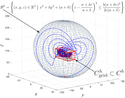
Figure 6: Localization of the hidden attractor of system (4) with $r=100$, $a=-9.965\cdot 10^{-3}$, $b=7.7454\cdot 10^{-2}$ by the absorbing set $\mathcal{B}^{h}$ with $\delta=-a+0.1$, cuboid $C^{h}=[-11,11]\times[-17,19]\times[80,117]$, and the corresponding grid of points $C^{h}_{\rm grid}$.

VI The finite-time Lyapunov dimension in the case of hidden attractor and multistability

Consider the dynamical system $\{\varphi^{t}\}_{t\geq 0}$ generated by system (4) with parameters (5) and its attractor $K$. Here $\varphi^{t}\big{(}(x_{0},y_{0},z_{0})\big{)}$ is a solution of (4) with the initial datum $(x_{0},y_{0},z_{0})$. Since the dynamical system $\{\varphi^{t}_{\rm R}\}_{t\geq 0}$, generated by the Rabinovich system (1), can be obtained from $\{\varphi^{t}\}_{t\geq 0}$ by the smooth transformation $\chi^{-1}$, inverse to (2), and inverse rescaling time (3) $t\to\nu_{1}t$, we have $\dim_{\rm L}(\{\varphi^{t}\}_{t\geq 0},K)=\dim_{\rm L}(\{\varphi^{t}_{\rm R}\}_{t\geq 0},\chi^{-1}(K))$. In our experiments, we consider system (4) with parameters $r=100$, $a=-9.965\cdot 10^{-3}$, $b=7.7454\cdot 10^{-2}$ corresponding to the hidden chaotic attractor.

Table 2: Numerical estimation of finite-time Lyapunov dimension in the case of hidden attractor (see Fig. 3)

	$t=100$
$u=(0,\,1,\,98)$	$t=100$
$u=(0.0099,\,0.0995,\,0)$	$t=100$
$\max_{u\in C^{h}_{\rm grid}}$	$\displaystyle\inf_{t\in[0,\,100]}\max_{u\in C^{h}_{\rm grid}}$
$\dim_{\rm L}(t,\,u)$ = ${\small{d}_{\rm L}^{\rm KY}(\{{\rm LE}_{i}(t,\,u)\}_{i=1}^{3})}$
	$2.1474$	$1.4987$	$2.2063$	$2.2050$
${\small{d}_{\rm L}^{\rm KY}(\{{\rm LCE}_{i}(t,\,u)\}_{i=1}^{3})}$
	$2.1338$	$1.1213$	$2.2105$	$2.2076$

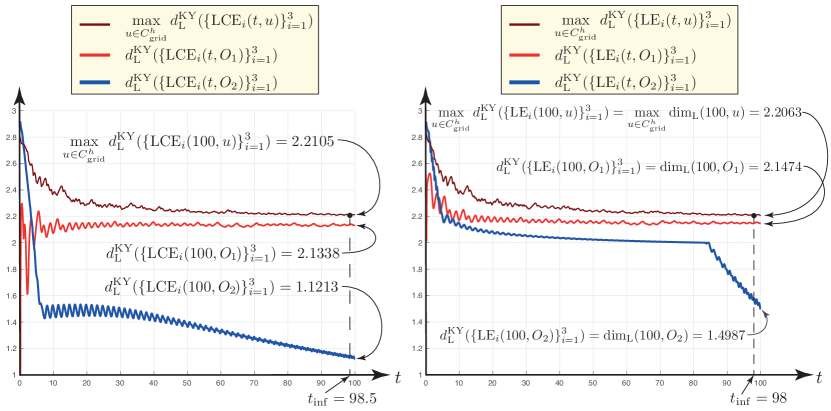
Figure 7: Dynamics of the finite-time local Lyapunov dimensions estimation on the time interval $t\in[0,100]$:
the maximum on the grid of points (dark red), at the point $O_{1}=(0,\,1,\,98)\in C^{h}_{\rm grid}$ (light red),
at the point $O_{2}=(0.0099,\,0.0995,\,0)$ from the one-dimensional unstable manifold of $S_{0}$ (blue).

In Fig. 6 it is shown the grid of points $C^{h}_{\rm grid}$ filling the hidden attractor: the grid of points fills cuboid $C^{h}=[-11,11]\times[-17,19]\times[80,117]$ with the distance between points equals to $0.5$. The time interval is $[0,\,T=100]$, $k=1000$, $\tau=0.1$, and the integration method is MATLAB ode45 with predefined parameters. The infimum on the time interval is computed at the points $\{t_{k}\}_{1}^{N}$ with time step $\tau=t_{i+1}-t_{i}=0.1$. Note that if for a certain time $t=t_{k}$ the computed trajectory is out of the cuboid, the corresponding value of finite-time local Lyapunov dimension is not taken into account in the computation of maximum of the finite-time local Lyapunov dimension (e.g. there are trajectories with initial data in cuboid, which are attracted to the zero equilibria, i.e. belong to its stable manifold, e.g. system (4) with $x=y=0$ is $\dot{z}=-bz$). For the finite-time Lyapunov exponents (FTLEs) computation we use MATLAB realization from LeonovKM-2015-EPJST based on (21) with $j=2$. For computation of the finite-time Lyapunov characteristic exponents (FTLCEs) we use MATLAB realization from KuznetsovMV-2014-CNSNS based on (23). For the considered set of parameters we compute:

1. finite-time local Lyapunov dimensions $\dim_{\rm L}(100,\cdot)$ at the point $O_{1}=(0,\,1,\,98)$, which belongs to the grid $C^{h}_{\rm grid}$, and at the point $O_{2}=(0.0099,\,0.0995,\,0)$ on the unstable manifold of zero equilibrium $S_{0}$;

2. maximum of the finite-time local Lyapunov dimensions at the points of grid, $\max_{u\in C^{h}_{\rm grid}}\dim_{\rm L}(t,u)$, for the time points $t=t_{k}=0.1\,k$ $(k=1,..,1000)$;

3. the corresponding values, given by the Kaplan-Yorke formula with respect to finite-time Lyapunov characteristic exponents.

The results are given in Table 2. The dynamics of finite-time local Lyapunov dimensions for different points and their maximums on a grid of points are shown in Fig. 7.

For the absorbing set $\mathcal{B}^{h}$ and the corresponding grid of points $\mathcal{B}^{h}_{\rm grid}$ (the distance between grid points is 5), by estimation (25) we get the following estimate:

$$\dim_{\rm H}K\leq\dim_{\rm L}K\leq\sup_{u\in\mathcal{B}^{h}}d_{\rm L}^{\rm KY}\big{(}\{\lambda_{j}(u)\}_{i=1}^{3}\big{)}\\ \approx\sup_{u\in\mathcal{B}^{h}_{\rm grid}}d_{\rm L}^{\rm KY}\big{(}\{\lambda_{j}(u)\}_{i=1}^{3}\big{)}=2.97001...\,.$$ (27)

Assuming $\sigma+1\geq b$, the eigenvalues of the unstable zero equilibrium $S_{0}$

$$\lambda_{1,3}(S_{0})=-\tfrac{1}{2}\left[(\sigma+1)\!\mp\!\sqrt{(\sigma-1)^{2}+4\sigma r}\right]\!,\,\lambda_{2}(S_{0})=-b$$

have the following order $\lambda_{1}(S_{0})>\lambda_{2}(S_{0})\geq\lambda_{3}(S_{0})$ and by (26) for the considered values of parameters we get

$$\dim_{\rm L}S_{0}=d_{\rm L}^{\rm KY}(\{\lambda_{i}(S_{0})\}_{i=1}^{3})=2+\tfrac{\lambda_{1}(S_{0})+\lambda_{2}(S_{0})}{|\lambda_{3}(S_{0})|}\\ \\ =3-\tfrac{2(\sigma+b+1)}{(\sigma+1)+\sqrt{(\sigma-1)^{2}+4\sigma r}}=2.8111...\ .$$ (28)

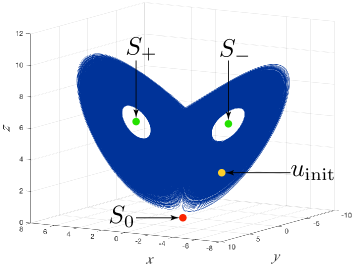
(a) Trajectory $u(t,u_{\rm init})$ for $t\in[0,\leavevmode\nobreak\ T_{1}]$,   $T_{1}\approx 15295$.

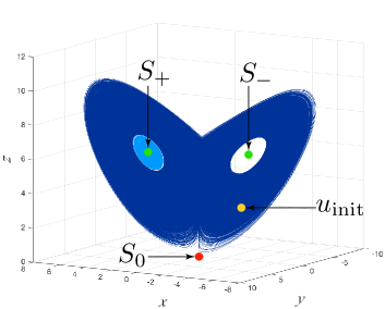
(b) Trajectory $u(t,u_{\rm init})$ for $t\in[0,\leavevmode\nobreak\ T]$,   $T=500000$

Figure 8: The trajectory forms a chaotic set, which looks like an “attractor” (navy blue) and then tends to $S_{+}$ (cyan).

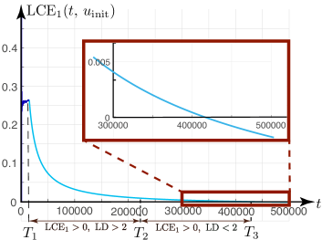
(a) $\operatorname{LCE}_{1}(t,\,u_{\rm init})$, $t\in[0,\leavevmode\nobreak\ T]$,   $T=5\cdot 10^{5}$.

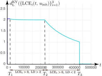
(b) ${d}_{\rm L}^{\rm KY}(\{\operatorname{LCE}_{i}(t,\,u_{\rm init})\}_{i=1}^{3})$, $t\in[0,\leavevmode\nobreak\ T]$,   $T=5\cdot 10^{5}$.

Figure 10: Numerical computation of $\operatorname{LCE}_{1}(t,\,u_{\rm init})$ and ${d}_{\rm L}^{\rm KY}(\{\operatorname{LCE}_{i}(t,\,u_{\rm init})\}_{i=1}^{3})$ for the time interval $[0,\,5\cdot 10^{5}]$.

The above numerical experiments lead to the following important remarks. While the Lyapunov dimension, unlike the Hausdorff dimension, is not a dimension in the rigorous sense HurewiczW-1941 (e.g. the Lyapunov dimension of the saddle point $S_{0}$ in (28) is noninteger), it gives an upper estimate of the Hausdorff dimension. If the attractor $K$ or the corresponding absorbing set $\mathcal{B}\supset K$ is known (see, e.g. (8)) and the purpose is to demonstrate that $\dim_{\rm H}K\leq\dim_{\rm L}K<3$, then it can be achieved without integration of the considered dynamical system (see, e.g. (27)). If the purpose is to get a precise estimation of the Hausdorff dimension, then one can use (18) and has to compute the finite-time Lyapunov dimension, i.e. to find the maximum of the finite-time local Lyapunov dimensions on a grid of points for a certain time. To be able to repeat a computation of finite-time Lyapunov dimension, one need to know the initial points of considered trajectories $\{u_{i}\}_{i=1}^{N}=K_{\rm grid}$ on the set $K$, time interval $(0,T]=\bigcup_{i=0}^{M-1}(t_{i},t_{i+1}]$, and the method of the finite-time Lyapunov estimation.

VII Computation of the Lyapunov dimension and transient chaos

Now we consider an example, which demonstrates difficulties in the reliable numerical computation of the Lyapunov dimension (i.e. numerical approximation of the limit value of the finite-time Lyapunov dimension).

Consider system (4) with parameters $r=6.485$, $a=-0.5$, $b=0.85$ for which equilibrium $S_{0}$ is a saddle point and equilibria $S_{\pm}$ are stable focus-nodes. We integrate numerically the trajectory with initial data $u_{0}=(0.5,\,0.5,\,0.5)$ in the vicinity of the $S_{0}$. We discard the part of the trajectory, corresponding to the initial transition process (for $[0,t_{\rm tp}=25000]$), and get the point $u_{\rm init}=($ $-2.089862710574761$, $-2.500837780529156$, $2.776106323157132).$ Further, we numerically approximate the finite-time Lyapunov exponents and dimension for the time interval $[0,\leavevmode\nobreak\ T]$ by Benettin’s algorithm (see approximation (23) and MATLAB code in (LET-1998, )).

The trajectory computed on the time interval $[0,T_{1}\approx 15295]$ traces a chaotic set in the phase space, which looks like an “attractor” (see Fig. 8a). Further integration with $t>T_{1}$ leads to the collapse of the “attractor” (see Fig. 8b), i.e. the “attractor” turns out to be a transient chaotic set. However on the time interval $t\in[0,\leavevmode\nobreak\ T_{3}\approx 431560]$ we have $\operatorname{LCE}_{1}(t,\,u_{\rm init})>0$ (see Fig. 10a) and, thus, one may conclude that the behavior is chaotic, and for the time interval $t\in[0,\leavevmode\nobreak\ T_{2}\approx 223447]$ we have ${d}_{\rm L}^{\rm KY}(\{\operatorname{LCE}_{i}(t,\,u_{\rm init})\}_{i=1}^{3})>2$ (see Fig. 10b). This effect is due to the fact that the finite-time Lyapunov exponents and finite-time Lyapunov dimension are averaged values over the considered time interval and, therefore, may reflect a change in the qualitative behavior of the trajectory with a delay. Since the lifetime of transient chaotic process can be extremely long and taking into account the limitations of reliable integration of chaotic ODEs, the long-time computation of the finite-time Lyapunov exponents and the finite-time Lyapunov dimension does not necessary lead to a more relevant approximation of the Lyapunov exponents and the Lyapunov dimension (see also effects in (24) for the approaches of Benettin et al. BenettinGGS-1980-Part2 and Wolf et al. WolfSSV-1985 ).

VIII Conclusion

In this work the Rabinovich system, describing the process of interaction between waves in plasma, is considered. We show that the methods of numerical continuation and perpetual point are helpful in localization and understanding of hidden attractor in the Rabinovich system. For the study of dimension of the hidden attractor the notion of the finite-time Lyapunov dimension is developed. An approach to reliable numerical estimation of the finite-time Lyapunov exponents (see relations (21)-(22)) and finite-time Lyapunov dimension (see relations (18)) is suggested. Various numerical estimates of the finite-time Lyapunov dimension for the hidden attractor in the case of multistability are given.

References

- (1) H. Poincare, Les methodes nouvelles de la mecanique celeste. Vol. 1-3, Gauthiers-Villars, Paris, 1892, 1893, 1899, [English transl. edited by D. Goroff: American Institute of Physics, NY, 1993].
- (2) A. M. Lyapunov, The General Problem of the Stability of Motion (in Russian), Kharkov, 1892, [English transl.: Academic Press, NY, 1966].
- (3) G. Leonov, V. Reitmann, Attraktoreingrenzung fur nichtlineare Systeme (in German), Teubner, Leipzig, 1987.
- (4) D. Hilbert, Mathematical problems, Bull. Amer. Math. Soc. (8) (1901-1902) 437–479.
- (5) G. Leonov, N. Kuznetsov, On differences and similarities in the analysis of Lorenz, Chen, and Lu systems, Applied Mathematics and Computation 256 (2015) 334–343. doi:10.1016/j.amc.2014.12.132.
- (6) A. Pisarchik, U. Feudel, Control of multistability, Physics Reports 540 (4) (2014) 167–218.
- (7) G. Leonov, N. Kuznetsov, Hidden attractors in dynamical systems. From hidden oscillations in Hilbert-Kolmogorov, Aizerman, and Kalman problems to hidden chaotic attractors in Chua circuits, International Journal of Bifurcation and Chaos 23 (1), art. no. 1330002. doi:10.1142/S0218127413300024.
- (8) N. Kuznetsov, G. Leonov, Hidden attractors in dynamical systems: systems with no equilibria, multistability and coexisting attractors, IFAC Proceedings Volumes 47 (2014) 5445–5454. doi:10.3182/20140824-6-ZA-1003.02501.
- (9) G. Leonov, N. Kuznetsov, T. Mokaev, Homoclinic orbits, and self-excited and hidden attractors in a Lorenz-like system describing convective fluid motion, Eur. Phys. J. Special Topics 224 (8) (2015) 1421–1458. doi:10.1140/epjst/e2015-02470-3.
- (10) N. Kuznetsov, Hidden attractors in fundamental problems and engineering models. A short survey, Lecture Notes in Electrical Engineering 371 (2016) 13–25, (Plenary lecture at International Conference on Advanced Engineering Theory and Applications 2015). doi:10.1007/978-3-319-27247-4\_2.
- (11) C. Grebogi, E. Ott, J. A. Yorke, Fractal basin boundaries, long-lived chaotic transients, and unstable-unstable pair bifurcation, Physical Review Letters 50 (13) (1983) 935.
- (12) D. Dudkowski, S. Jafari, T. Kapitaniak, N. Kuznetsov, G. Leonov, A. Prasad, Hidden attractors in dynamical systems, Physics Reports 637 (2016) 1–50. doi:10.1016/j.physrep.2016.05.002.
- (13) J. Kaplan, J. Yorke, Chaotic behavior of multidimensional difference equations, in: Functional Differential Equations and Approximations of Fixed Points, Springer, Berlin, 1979, pp. 204–227.
- (14) P. Grassberger, I. Procaccia, Measuring the strangeness of strange attractors, Physica D: Nonlinear Phenomena 9 (1-2) (1983) 189–208.
- (15) J.-P. Eckmann, D. Ruelle, Ergodic theory of chaos and strange attractors, Reviews of Modern Physics 57 (3) (1985) 617–656.
- (16) P. Constantin, C. Foias, R. Temam, Attractors representing turbulent flows, Memoirs of the American Mathematical Society 53 (314) (1985) 1–67.
- (17) H. Abarbanel, R. Brown, J. Sidorowich, L. Tsimring, The analysis of observed chaotic data in physical systems, Reviews of Modern Physics 65 (4) (1993) 1331–1392.
- (18) V. Boichenko, G. Leonov, V. Reitmann, Dimension Theory for Ordinary Differential Equations, Teubner, Stuttgart, 2005.
- (19) N. Kuznetsov, The Lyapunov dimension and its estimation via the Leonov method, Physics Letters A 380 (25–26) (2016) 2142–2149. doi:10.1016/j.physleta.2016.04.036.
- (20) M. I. Rabinovich, Stochastic autooscillations and turbulence, Uspehi Physicheskih Nauk 125 (1) (1978) 123–168.
- (21) A. Pikovski, M. Rabinovich, V. Trakhtengerts, Onset of stochasticity in decay confinement of parametric instability, Sov. Phys. JETP 47 (1978) 715–719.
- (22) G. Leonov, V. Boichenko, Lyapunov’s direct method in the estimation of the Hausdorff dimension of attractors, Acta Applicandae Mathematicae 26 (1) (1992) 1–60.
- (23) E. N. Lorenz, Deterministic nonperiodic flow, J. Atmos. Sci. 20 (2) (1963) 130–141.
- (24) I. Chueshov, Introduction to the Theory of Infinite-dimensional Dissipative Systems, Electronic library of mathematics, ACTA, 2002.
- (25) G. Leonov, N. Kuznetsov, V. Vagaitsev, Localization of hidden Chua’s attractors, Physics Letters A 375 (23) (2011) 2230–2233. doi:10.1016/j.physleta.2011.04.037.
- (26) H. Barkhausen, Textbook of Electron Tubes and their Technical Applications (in German), S. Hirzel, Leipzig, 1935.
- (27) L. Mandelstam, N. Papalexi, Über resonanzerscheinungen bei frequenzteilung, Zeitschrift für Physik (in German) 73 (3) (1932) 223–248. doi:10.1007/BF01351217.
- (28) A. A. Andronov, E. A. Vitt, S. E. Khaikin, Theory of Oscillators (in Russian), ONTI NKTP SSSR, 1937, [English transl.: 1966, Pergamon Press].
- (29) A. Jenkins, Self-oscillation, Physics Reports 525 (2) (2013) 167–222.
- (30) A. Sommerfeld, Beitrage zum dynamischen ausbau der festigkeitslehre, Zeitschrift des Vereins deutscher Ingenieure (in German) 46 (1902) 391–394.
- (31) M. Kiseleva, N. Kuznetsov, G. Leonov, Hidden attractors in electromechanical systems with and without equilibria, IFAC-PapersOnLine 49 (14) (2016) 51–55. doi:10.1016/j.ifacol.2016.07.975.
- (32) G. Leonov, N. Kuznetsov, Algorithms for searching for hidden oscillations in the Aizerman and Kalman problems, Doklady Mathematics 84 (1) (2011) 475–481. doi:10.1134/S1064562411040120.
- (33) M. A. Aizerman, On a problem concerning the stability in the large of dynamical systems, Uspekhi Mat. Nauk (in Russian) 4 (1949) 187–188.
- (34) R. E. Kalman, Physical and mathematical mechanisms of instability in nonlinear automatic control systems, Transactions of ASME 79 (3) (1957) 553–566.
- (35) N. N. Bautin, On the number of limit cycles generated on varying the coefficients from a focus or centre type equilibrium state, Doklady Akademii Nauk SSSR (in Russian) 24 (7) (1939) 668–671.
- (36) N. Kuznetsov, O. Kuznetsova, G. Leonov, Visualization of four normal size limit cycles in two-dimensional polynomial quadratic system, Differential equations and dynamical systems 21 (1-2) (2013) 29–34. doi:10.1007/s12591-012-0118-6.
- (37) N. Kuznetsov, G. Leonov, V. Vagaitsev, Analytical-numerical method for attractor localization of generalized Chua’s system, IFAC Proceedings Volumes 43 (11) (2010) 29–33. doi:10.3182/20100826-3-TR-4016.00009.
- (38) V. Bragin, V. Vagaitsev, N. Kuznetsov, G. Leonov, Algorithms for finding hidden oscillations in nonlinear systems. The Aizerman and Kalman conjectures and Chua’s circuits, Journal of Computer and Systems Sciences International 50 (4) (2011) 511–543. doi:10.1134/S106423071104006X.
- (39) G. Leonov, N. Kuznetsov, V. Vagaitsev, Hidden attractor in smooth Chua systems, Physica D: Nonlinear Phenomena 241 (18) (2012) 1482–1486. doi:10.1016/j.physd.2012.05.016.
- (40) N. Kuznetsov, O. Kuznetsova, G. Leonov, V. Vagaitsev, Analytical-numerical localization of hidden attractor in electrical Chua’s circuit, Lecture Notes in Electrical Engineering 174 (4) (2013) 149–158. doi:10.1007/978-3-642-31353-0\_11.
- (41) M. Kiseleva, E. Kudryashova, N. Kuznetsov, O. Kuznetsova, G. Leonov, M. Yuldashev, R. Yuldashev, Hidden and self-excited attractors in Chua circuit: synchronization and SPICE simulation, International Journal of Parallel, Emergent and Distributed Systems (2017) 1–11 doi:10.1080/17445760.2017.1334776.
- (42) N. Stankevich, N. Kuznetsov, G. Leonov, L. Chua, Scenario of the birth of hidden attractors in the Chua circuit, International Journal of Bifurcation and Chaos 27 (12), accepted.
- (43) I. Burkin, N. Khien, Analytical-numerical methods of finding hidden oscillations in multidimensional dynamical systems, Differential Equations 50 (13) (2014) 1695–1717.
- (44) C. Li, J. Sprott, Coexisting hidden attractors in a 4-D simplified Lorenz system, International Journal of Bifurcation and Chaos 24 (03), art. num. 1450034.
- (45) Q. Li, H. Zeng, X.-S. Yang, On hidden twin attractors and bifurcation in the Chua’s circuit, Nonlinear Dynamics 77 (1-2) (2014) 255–266.
- (46) V.-T. Pham, F. Rahma, M. Frasca, L. Fortuna, Dynamics and synchronization of a novel hyperchaotic system without equilibrium, International Journal of Bifurcation and Chaos 24 (06), art. num. 1450087.
- (47) M. Chen, M. Li, Q. Yu, B. Bao, Q. Xu, J. Wang, Dynamics of self-excited attractors and hidden attractors in generalized memristor-based Chua’s circuit, Nonlinear Dynamics 81 (2015) 215–226.
- (48) A. Kuznetsov, S. Kuznetsov, E. Mosekilde, N. Stankevich, Co-existing hidden attractors in a radio-physical oscillator system, Journal of Physics A: Mathematical and Theoretical 48 (2015) 125101.
- (49) P. Saha, D. Saha, A. Ray, A. Chowdhury, Memristive non-linear system and hidden attractor, European Physical Journal: Special Topics 224 (8) (2015) 1563–1574.
- (50) V. Semenov, I. Korneev, P. Arinushkin, G. Strelkova, T. Vadivasova, V. Anishchenko, Numerical and experimental studies of attractors in memristor-based Chua’s oscillator with a line of equilibria. Noise-induced effects, European Physical Journal: Special Topics 224 (8) (2015) 1553–1561.
- (51) P. Sharma, M. Shrimali, A. Prasad, N. Kuznetsov, G. Leonov, Control of multistability in hidden attractors, Eur. Phys. J. Special Topics 224 (8) (2015) 1485–1491.
- (52) Z. Zhusubaliyev, E. Mosekilde, A. Churilov, A. Medvedev, Multistability and hidden attractors in an impulsive Goodwin oscillator with time delay, European Physical Journal: Special Topics 224 (8) (2015) 1519–1539.
- (53) M.-F. Danca, N. Kuznetsov, G. Chen, Unusual dynamics and hidden attractors of the Rabinovich–Fabrikant system, Nonlinear Dynamics 88 (2017) 791–805. doi:10.1007/s11071-016-3276-1.
- (54) S. Jafari, V.-T. Pham, S. Golpayegani, M. Moghtadaei, S. Kingni, The relationship between chaotic maps and some chaotic systems with hidden attractors, Int. J. Bifurcat. Chaos 26 (13), art. num. 1650211.
- (55) T. Menacer, R. Lozi, L. Chua, Hidden bifurcations in the multispiral Chua attractor, International Journal of Bifurcation and Chaos 26 (14), art. num. 1630039.
- (56) O. Ojoniyi, A. Njah, A 5D hyperchaotic Sprott B system with coexisting hidden attractors, Chaos, Solitons & Fractals 87 (2016) 172–181.
- (57) V.-T. Pham, C. Volos, S. Jafari, S. Vaidyanathan, T. Kapitaniak, X. Wang, A chaotic system with different families of hidden attractors, International Journal of Bifurcation and Chaos 26 (08) (2016) 1650139.
- (58) R. Rocha, R. O. Medrano-T, Finding hidden oscillations in the operation of nonlinear electronic circuits, Electronics Letters 52 (12) (2016) 1010–1011.
- (59) Z. Wei, V.-T. Pham, T. Kapitaniak, Z. Wang, Bifurcation analysis and circuit realization for multiple-delayed Wang–Chen system with hidden chaotic attractors, Nonlinear Dynamics 85 (3) (2016) 1635–1650.
- (60) I. Zelinka, Evolutionary identification of hidden chaotic attractors, Engineering Applications of Artificial Intelligence 50 (2016) 159–167.
- (61) M. Borah, B. Roy, Hidden attractor dynamics of a novel non-equilibrium fractional-order chaotic system and its synchronisation control, in: 2017 Indian Control Conference (ICC), 2017, pp. 450–455.
- (62) P. Brzeski, J. Wojewoda, T. Kapitaniak, J. Kurths, P. Perlikowski, Sample-based approach can outperform the classical dynamical analysis - experimental confirmation of the basin stability method, Scientific Reports 7, art. num. 6121.
- (63) Y. Feng, W. Pan, Hidden attractors without equilibrium and adaptive reduced-order function projective synchronization from hyperchaotic Rikitake system, Pramana 88 (4) (2017) 62.
- (64) H. Jiang, Y. Liu, Z. Wei, L. Zhang, Hidden chaotic attractors in a class of two-dimensional maps, Nonlinear Dynamics 85 (4) (2016) 2719–2727.
- (65) N. Kuznetsov, G. Leonov, M. Yuldashev, R. Yuldashev, Hidden attractors in dynamical models of phase-locked loop circuits: limitations of simulation in MATLAB and SPICE, Commun Nonlinear Sci Numer Simulat 51 (2017) 39–49. doi:10.1016/j.cnsns.2017.03.010.
- (66) J. Ma, F. Wu, W. Jin, P. Zhou, T. Hayat, Calculation of Hamilton energy and control of dynamical systems with different types of attractors, Chaos: An Interdisciplinary Journal of Nonlinear Science 27 (5) (2017) 053108. doi:10.1063/1.4983469.
- (67) M. Messias, A. Reinol, On the formation of hidden chaotic attractors and nested invariant tori in the Sprott A system, Nonlinear Dynamics 88 (2) (2017) 807–821.
- (68) J. Singh, B. Roy, Multistability and hidden chaotic attractors in a new simple 4-D chaotic system with chaotic 2-torus behaviour, International Journal of Dynamics and Control doi: 10.1007/s40435-017-0332-8.
- (69) C. Volos, V.-T. Pham, E. Zambrano-Serrano, J. M. Munoz-Pacheco, S. Vaidyanathan, E. Tlelo-Cuautle, Advances in Memristors, Memristive Devices and Systems, Springer, 2017, Ch. Analysis of a 4-D hyperchaotic fractional-order memristive system with hidden attractors, pp. 207–235.
- (70) Z. Wei, I. Moroz, J. Sprott, A. Akgul, W. Zhang, Hidden hyperchaos and electronic circuit application in a 5D self-exciting homopolar disc dynamo, Chaos 27 (3), art. num. 033101.
- (71) G. Zhang, F. Wu, C. Wang, J. Ma, Synchronization behaviors of coupled systems composed of hidden attractors, International Journal of Modern Physics B 31, art. num. 1750180.
- (72) Y. Lai, T. Tel, Transient Chaos: Complex Dynamics on Finite Time Scales, Springer, New York, 2011.
- (73) M.-F. Danca, N. Kuznetsov, Hidden chaotic sets in a Hopfield neural system, Chaos, Solitons & Fractals 103 (2017) 144–150. doi:https://doi.org/10.1016/j.chaos.2017.06.002.
- (74) G. Chen, N. Kuznetsov, G. Leonov, T. Mokaev, Hidden attractors on one path: Glukhovsky-Dolzhansky, Lorenz, and Rabinovich systems, International Journal of Bifurcation and Chaos 27 (8), art. num. 1750115.
- (75) N. Kuznetsov, G. Leonov, T. Mokaev, S. Seledzhi, Hidden attractor in the Rabinovich system, Chua circuits and PLL, AIP Conference Proceedings 1738 (1), art. num. 210008.
- (76) G. Leonov, N. Kuznetsov, T. Mokaev, Hidden attractor and homoclinic orbit in Lorenz-like system describing convective fluid motion in rotating cavity, Communications in Nonlinear Science and Numerical Simulation 28 (2015) 166–174. doi:10.1016/j.cnsns.2015.04.007.
- (77) A. Prasad, Existence of perpetual points in nonlinear dynamical systems and its applications, International Journal of Bifurcation and Chaos 25 (2), art. num. 1530005.
- (78) D. Dudkowski, A. Prasad, T. Kapitaniak, Perpetual points and hidden attractors in dynamical systems, Physics Letters A 379 (40-41) (2015) 2591 – 2596.
- (79) A. Prasad, A note on topological conjugacy for perpetual points, International Journal of Nonlinear Science 21 (1) (2016) 60–64.
- (80) F. Nazarimehr, B. Saedi, S. Jafari, J. Sprott, Are perpetual points sufficient for locating hidden attractors?, International Journal of Bifurcation and Chaos 27 (03), art. num. 1750037.
- (81) A. Douady, J. Oesterle, Dimension de Hausdorff des attracteurs, C.R. Acad. Sci. Paris, Ser. A. (in French) 290 (24) (1980) 1135–1138.
- (82) B. Hunt, Maximum local Lyapunov dimension bounds the box dimension of chaotic attractors, Nonlinearity 9 (4) (1996) 845–852.
- (83) M. Rabinovich, A. Ezersky, P. Weidman, The Dynamics of Patterns, World Scientific, 2000.
- (84) N. Kuznetsov, T. Alexeeva, G. Leonov, Invariance of Lyapunov exponents and Lyapunov dimension for regular and irregular linearizations, Nonlinear Dynamics 85 (1) (2016) 195–201. doi:10.1007/s11071-016-2678-4.
- (85) F. Ledrappier, Some relations between dimension and Lyapounov exponents, Communications in Mathematical Physics 81 (2) (1981) 229–238.
- (86) P. Frederickson, J. Kaplan, E. Yorke, J. Yorke, The Liapunov dimension of strange attractors, Journal of Differential Equations 49 (2) (1983) 185–207.
- (87) J. Farmer, E. Ott, J. Yorke, The dimension of chaotic attractors, Physica D: Nonlinear Phenomena 7 (1-3) (1983) 153 – 180.
- (88) N. Bogoliubov, N. Krylov, La theorie generalie de la mesure dans son application a l’etude de systemes dynamiques de la mecanique non-lineaire, Ann. Math. II (in French) (Annals of Mathematics) 38 (1) (1937) 65–113.
- (89) M. Dellnitz, O. Junge, Set oriented numerical methods for dynamical systems, in: Handbook of Dynamical Systems, Vol. 2, Elsevier Science, 2002, pp. 221–264.
- (90) V. Oseledets, A multiplicative ergodic theorem. Characteristic Ljapunov, exponents of dynamical systems, Trudy Moskovskogo Matematicheskogo Obshchestva (in Russian) 19 (1968) 179–210.
- (91) L. Barreira, J. Schmeling, Sets of “Non-typical” points have full topological entropy and full Hausdorff dimension, Israel Journal of Mathematics 116 (1) (2000) 29–70.
- (92) P. Cvitanović, R. Artuso, R. Mainieri, G. Tanner, G. Vattay, Chaos: Classical and Quantum, Niels Bohr Institute, Copenhagen, 2016, http://ChaosBook.org.
- (93) W. Ott, J. Yorke, When Lyapunov exponents fail to exist, Phys. Rev. E 78 (2008) 056203.
- (94) L.-S. Young, Mathematical theory of Lyapunov exponents, Journal of Physics A: Mathematical and Theoretical 46 (25) (2013) 254001.
- (95) A. Pikovsky, A. Politi, Lyapunov Exponents: A Tool to Explore Complex Dynamics, Cambridge University Press, 2016.
- (96) N. Kuznetsov, G. Leonov, On stability by the first approximation for discrete systems, in: 2005 International Conference on Physics and Control, PhysCon 2005, Vol. Proceedings Volume 2005, IEEE, 2005, pp. 596–599. doi:10.1109/PHYCON.2005.1514053.
- (97) G. Leonov, N. Kuznetsov, Time-varying linearization and the Perron effects, International Journal of Bifurcation and Chaos 17 (4) (2007) 1079–1107. doi:10.1142/S0218127407017732.
- (98) J. Schmeling, A dimension formula for endomorphisms – the Belykh family, Ergodic Theory and Dynamical Systems 18 (1998) 1283–1309.
- (99) J. Vallejo, M. Sanjuan, Predictability of Chaotic Dynamics: A Finite-time Lyapunov Exponents Approach, Springer International Publishing, 2017.
- (100) B. Kehlet, A. Logg, Quantifying the computability of the Lorenz system using a posteriori analysis, in: Proceedings of the VI Int. conf. on Adaptive Modeling and Simulation (ADMOS 2013), 2013.
- (101) B. Kehlet, A. Logg, A posteriori error analysis of round-off errors in the numerical solution of ordinary differential equations, Numerical Algorithms (2015) 1–20.
- (102) S. Liao, P. Wang, On the mathematically reliable long-term simulation of chaotic solutions of Lorenz equation in the interval [0,10000], Science China Physics, Mechanics and Astronomy 57 (2) (2014) 330–335.
- (103) A. Eden, An abstract theory of L-exponents with applications to dimension analysis (PhD thesis), Indiana University, 1989.
- (104) K. Ramasubramanian, M. Sriram, A comparative study of computation of Lyapunov spectra with different algorithms, Physica D: Nonlinear Phenomena 139 (1-2) (2000) 72–86.
- (105) H. Rutishauser, H. Schwarz, The LR transformation method for symmetric matrices, Numerische Mathematik 5 (1) (1963) 273–289.
- (106) D. Stewart, A new algorithm for the SVD of a long product of matrices and the stability of products, Electronic Transactions on Numerical Analysis 5 (1997) 29–47.
- (107) G. Benettin, L. Galgani, A. Giorgilli, J.-M. Strelcyn, Lyapunov characteristic exponents for smooth dynamical systems and for hamiltonian systems. A method for computing all of them. Part 2: Numerical application, Meccanica 15 (1) (1980) 21–30.
- (108) A. Wolf, J. B. Swift, H. L. Swinney, J. A. Vastano, Determining Lyapunov exponents from a time series, Physica D: Nonlinear Phenomena 16 (D) (1985) 285–317.
- (109) B. E. Bylov, R. E. Vinograd, D. M. Grobman, V. V. Nemytskii, Theory of characteristic exponents and its applications to problems of stability (in Russian), Nauka, Moscow, 1966.
- (110) R. Smith, Some application of Hausdorff dimension inequalities for ordinary differential equation, Proc. Royal Society Edinburg 104A (1986) 235–259.
- (111) C. Doering, J. Gibbon, D. Holm, B. Nicolaenko, Exact Lyapunov dimension of the universal attractor for the complex Ginzburg-Landau equation, Phys. Rev. Lett. 59 (1987) 2911–2914.
- (112) N. Kuznetsov, G. Leonov, A short survey on Lyapunov dimension for finite dimensional dynamical systems in Euclidean space, arXiv https://arxiv.org/pdf/1510.03835.pdf.
- (113) G. Leonov, On estimations of Hausdorff dimension of attractors, Vestnik St. Petersburg University: Mathematics 24 (3) (1991) 38–41, [Transl. from Russian: Vestnik Leningradskogo Universiteta. Mathematika, 24(3), 1991, pp. 41-44].
- (114) V. Boichenko, G. Leonov, Lyapunov’s direct method in estimates of topological entropy, Journal of Mathematical Sciences 91 (6) (1998) 3370–3379.
- (115) A. Y. Pogromsky, A. S. Matveev, Estimation of topological entropy via the direct Lyapunov method, Nonlinearity 24 (7) (2011) 1937–1959.
- (116) N. Kuznetsov, T. Mokaev, P. Vasilyev, Numerical justification of Leonov conjecture on Lyapunov dimension of Rossler attractor, Commun Nonlinear Sci Numer Simulat 19 (2014) 1027–1034.
- (117) W. Hurewicz, H. Wallman, Dimension Theory, Princeton University Press, Princeton, 1941.
- (118) S. Siu, www.mathworks.com/matlabcentral/fileexchange/233-let (1998).