A Unified Energy-Reservoir Model Containing Contributions from ⁵⁶Ni and Neutron Stars and Its Implication to Luminous Type Ic Supernovae

Abstract

Most type-Ic core-collapse supernovae (CCSNe) produce ⁵⁶Ni and neutron stars (NSs) or black holes (BHs). The dipole radiation of nascent NSs has usually been neglected in explaining supernovae (SNe) with peak absolute magnitude $M_{\rm peak}$ in any band are $\gtrsim-19.5$ mag, while the ⁵⁶Ni can be neglected in fitting most type-Ic superluminous supernovae (SLSNe Ic) whose $M_{\rm peak}$ in any band are $\lesssim-21$ mag, since the luminosity from a magnetar (highly magnetized NS) can outshine that from a moderate amount of ⁵⁶Ni. For luminous SNe Ic with $-21\lesssim M_{\rm peak}\lesssim-19.5$ mag, however, both contributions from ⁵⁶Ni and NSs cannot be neglected without serious modeling, since they are not SLSNe and the ⁵⁶Ni mass could be up to $\sim 0.5M_{\odot}$. In this paper we propose a unified model that contain contributions from both ⁵⁶Ni and a nascent NS. We select three luminous SNe Ic-BL, SN 2010ay, SN 2006nx, and SN 14475, and show that, if these SNe are powered by ⁵⁶Ni, the ratio of $M_{\rm Ni}$ to $M_{\rm ej}$ are unrealistic. Alternatively, we invoke the magnetar model and the hybrid (⁵⁶Ni + NS) model and find that they can fit the observations, indicating that our models are valid and necessary for luminous SNe Ic. Owing to the lack of late-time photometric data, we cannot break the parameter degeneracy and thus distinguish among the model parameters, but we can expect that future multi-epoch observations of luminous SNe can provide stringent constraints on ⁵⁶Ni yields and the parameters of putative magnetars.

1 Introduction

It has long been believed that most aged massive (zero-age main-sequence mass $M_{\rm ZAMS}\gtrsim 8.0M_{\odot}$) stars terminate their lives as core-collapse supernovae (CCSNe) (Woosley et al., 2002; Janka et al., 2007), which are classified into type IIP, IIL, IIn, IIb, Ib and Ic according to their spectra and light curves (Filippenko, 1997), leaving neutron stars (NSs) or black holes (BHs) at the center and producing a moderate amount of ⁵⁶Ni which is generally regarded as the dominant power source for most supernovae (SNe) (Colgate & McKee, 1969; Colgate et al., 1980; Arnett, 1982) . Of all these subclasses, SNe Ic have attracted more and more attentions since a great number of these events have been discovered and confirmed in recent years that some SNe Ic with broad absorption line features (“broad-lined” or “BL”) have an accompanying gamma-ray burst (GRB) or X-ray flash (XRF) (Woosley & Bloom, 2006; Hjorth & Bloom, 2012). Main models of central engines of GRBs associated with SNe are the “collapsar” model (Woosley, 1993; MacFadyen & Woosley, 1999) involving “BH + disk” systems and the magnetar (highly magnetized neutron star) model (Usov, 1992; Metzger et al., 2007; Bucciantini et al., 2008; Metzger et al., 2011) proposing that the explosions may leave benind fast-rotating magnetars, being also regarded as the origin of the shallow decays and plateaus as well as rebrightenings in the multi-band afterglows of some GRBs (Dai & Lu, 1998a, b; Zhang & Mészáros, 2001; Dai, 2004; Dai & Liu, 2012).

On the other hand, in the last two decades, optical$-$NIR and radio observations have revealed that not every SN Ic-BL associates with a GRB or an XRF (Soderberg et al., 2005; Drout et al., 2011). Many SNe Ic-BL, no matter whether they are associated a(n) GRB/XRF or not, have very high kinetic energy $E_{\rm K}\gtrsim 1.0\times 10^{52}$ erg and have therefore been called “Hypernovae” (Iwamoto et al., 1998). Supposing that the optical$-$NIR emission is powered by radioactive ⁵⁶Ni decay, these SNe Ic need $\sim 0.1-0.5M_{\odot}$ of ⁵⁶Ni. All GRBs associated SNe Ic and most GRB-less SNe Ic are not very luminous, with peak absolute magnitude $M_{\rm peak}\gtrsim-19.5$.

Thanks to the unprecedented boom of targeted- and untargeted- sky survey programs, many superluminous SNe (SLSNe) whose $M_{\rm peak}$ in any band are $\lesssim-21$ mag (Gal-Yam, 2012) have been found in the past decade, most of which cannot be explained by the widely adopted ⁵⁶Ni decay model (Quimby et al., 2011; Inserra et al., 2013; Nicholl et al., 2013; McCrum et al., 2014; Nicholl et al., 2014), motivating researchers to consider alternative energy-reservoir models. Currently, main models explaining the SLSNe are SN ejecta - circumstellar medium (CSM) interaction model (Chevalier, 1982; Chevalier & Fransson, 1994; Chevalier & Irwin, 2011; Ginzburg & Balberg, 2012) that has been employed to explain many Type IIn luminous SNe (Chugai, 1994; Zhang et al., 2012; Ofek et al., 2013) and superluminous SNe IIn (Smith & McCray, 2007; Moriya et al., 2013) as well as some Type Ic SLSNe (Chatzopoulos et al., 2013; Nicholl et al., 2014), and the magnetar-powered SLSNe model (Kasen & Bildsten, 2010; Woosley, 2010) that has been used to explain many Type Ic SLSNe (Inserra et al., 2013; Nicholl et al., 2013; Howell et al., 2013; McCrum et al., 2014; Vreeswijk et al., 2014; Nicholl et al., 2014; Wang et al., 2015). In some cases, the magnetar-powered SLSNe model with the assumption of full energy trapping fails to fit the late-time light curves (Inserra et al., 2013; Nicholl et al., 2014). In Wang et al. (2015), we generalized the magnetar-powered SLSNe model by introducing the hard emission leakage and solved this problem, highlighting the importance of the leakage effect in this model.

Thus, the power sources of most normal SNe and SLSNe have been attributed to ⁵⁶Ni-decay and the magnetar spin-down or ejecta-CSM interaction, respectively. Within this picture, the dipole radiation of nascent magnetars has usually been neglected in explaining the SNe with $M_{\rm peak}\gtrsim-19.5$ (but see Maeda et al., 2007), while the ⁵⁶Ni decay energy have generally been ignored in fitting all Type Ic SLSNe ($M_{\rm peak}\lesssim-21$) because the peak-luminosity due to the energy injection from a newly born fast-rotating (initial period $\sim$ millisecond) magnetar can outshine that from a moderate amount of ⁵⁶Ni (see Inserra et al., 2013, for further analysis).

Besides normal SNe and SLSNe mentioned above, however, there are some SNe with $-21\lesssim M_{\rm peak}\lesssim-19.5$ mag, constituting a class of “gap-filler” events that bridge normal SNe and SLSNe, have been found by many telescopes. Most of these “gap-filler” SNe are explained by the ⁵⁶Ni decay model for SNe Ic as well as “Super-Chandrasekhar-Mass” SNe Ia, and the ejecta-CSM interaction model for SNe IIn.

Among these “gap-filler” SNe with $-21\lesssim M_{\rm peak}\lesssim-19.5$ mag, luminous Type Ic SNe and their energy-reservoir mechanisms have not attracted enough attentions yet, their high peak-luminosities are simply attributed to the ⁵⁶Ni cascade decay without any detailed modeling. It has recently been demonstrated that the ⁵⁶Ni-decay model cannot be arbitrarily used to explain all SNe Ic especially those very luminous ones (Inserra et al., 2013; Nicholl et al., 2013) since the production of ⁵⁶Ni is ineffective in CCSNe and more ⁵⁶Ni mass needs more mass of the ejecta, which could theoretically result in broad light curves that usually conflict with observations. While the CSM-interaction model can predict a wide range of peak luminosities and therefore explain the normal, luminous, and superluminous SNe IIn as a whole category, ⁵⁶Ni-decay model cannot explain luminous SNe Ic.

Here, we propose that for some luminous SNe Ic, there are other energy reservoirs that play a significant role in producing light curves. Since all hydrogen envelopes of progenitors of SNe Ic have been stripped and the spectra are lack of narrow and/or emission lines indicative of the interactions , we can exclude the ionized hydrogen re-combination (Falk & Arnett, 1977; Klein & Chevalier, 1978; Popov, 1993; Kasen & Woosley, 2009) and do not consider the ejecta-CSM interaction process. Therefore, like the cases of SLSNe Ic, the nascent magnetar embedded in the center of the explosion is the most promising candidate for the additional power source (Ostriker & Gunn, 1971). On the other hand, the production of ⁵⁶Ni is inevitable and cannot be neglected in modeling luminous SNe Ic because their peak luminosities are considerably lower than that of SLSNe and the contributions from a moderate amount of ⁵⁶Ni can be comparable with the contributions given by any other energy reservoirs. Furthermore, in principle, the contributions from ⁵⁶Ni and NSs cannot be directly neglected for CCSNe with a wide range of peak luminosities. Thus, it is necessary to consider a unified model containing contributions from both ⁵⁶Ni and NSs.

In this paper we construct the unified model which contain the contributions from both the ⁵⁶Ni cascade decay energy and the NS rotational energy, and apply it to explain the light curves of some luminous SNe Ic-BL, i.e., SN 2010ay, SN 2006nx, and SN 14475. The remainder of this paper is organized as follows. In Section 2, we give a unified semi-analytical model for Type Ic SNe. Based on this model, we fit the light curves of SN 2010ay, SN 2006nx, and SN 14475 in Section 3. Finally, some discussions and conclusions are presented in Section 4.

2 The unified semi-analytical model for SNe

In this section, we construct a unified semi-analytical model combining energy from a spin-down magnetar and an amount of ⁵⁶Ni to describe the SN luminosity evolution. In this unified model, ⁵⁶Ni release high energy photons via the cascade decay chain ⁵⁶Ni$\rightarrow$⁵⁶Co$\rightarrow$⁵⁶Fe, while the magnetar can inject its rotational energy into the SN ejecta as heat energy (Ostriker & Gunn, 1971).

Based on Arnett (1982), taking into account the $\gamma$-ray and X-ray leakage (e.g., Clocchiatti & Wheeler, 1997; Valenti et al., 2008; Chatzopoulos et al., 2009, 2012; Drout et al., 2013; Wang et al., 2015), the luminosity is given by

$$L(t) = \frac{2}{\tau_{m}}e^{-\left(\frac{t^{2}}{\tau_{m}^{2}}+\frac{2R_{0}t}{v\tau_{m}^{2}}\right)}~{}\left(1-e^{-\tau_{\gamma}(t)}\right)\int_{0}^{t}e^{\left(\frac{t^{\prime 2}}{\tau_{m}^{2}}+\frac{2R_{0}t^{\prime}}{v\tau_{m}^{2}}\right)}$$ (1)

$$\times\left(\frac{R_{0}}{v\tau_{m}}+\frac{t^{\prime}}{\tau_{m}}\right)P(t^{\prime})dt^{\prime}~{}\mbox{erg s}^{-1},$$

where $R_{0}$ is the initial radius of the progenitor, which is very small compared to the radius of the ejecta. We take the limit $R_{0}\rightarrow 0$, then the above equation can be largely simplified. With Equations (18), (19) and (22) of Arnett (1982), the effective light-curve timescale $\tau_{m}$ can be written as

$$\tau_{m}=\left(\frac{2\kappa M_{\rm ej}}{\beta vc}\right)^{1/2},$$ (2)

where $\kappa$ is the optical opacity to optical photons (i.e., the Thomson electron scattering opacity), $M_{\rm ej}$ and $v$ are the mass and expansion speed of the ejecta, respectively, and $c$ is the speed of light. $\beta\simeq 13.8$ is a constant that accounts for the density distribution of the ejecta. $P(t)$ is the power function. Here, $v$ is the scale velocity ($v_{\rm sc}$) in Arnett (1982) and approximates to the photospheric expansion velocity $v_{\rm ph}$. Hereafter, we let $v\simeq v_{\rm ph}$.

The factors $e^{-\tau_{\gamma}(t)}$ and $(1-e^{-\tau_{\gamma}(t)})$ in Equation (1) represent the $\gamma$-ray leakage and trapping rate, respectively. $\tau_{\gamma}(t)~{}=~{}At^{-2}$ is the optical depth to $\gamma$-rays (Chatzopoulos et al., 2009, 2012). If the SN ejecta has a uniform density distribution ($M_{\rm ej}~{}=~{}(4/3)\pi\rho R^{3}$, $E_{\rm K}~{}=~{}(3/10)M_{\rm ej}v^{2}$), $A$ depends on $\kappa_{\gamma}$ (the opacity to $\gamma$-rays), $M_{\rm ej}$ and $v$ as

$$A = \frac{3\kappa_{\gamma}M_{\rm ej}}{4\pi v^{2}}$$ (3)

$$= 4.75\times 10^{13}\left(\frac{\kappa_{\gamma}}{0.1~{}{\rm cm}^{2}~{}{\rm g}^{-1}}\right)$$

$$\times\left(\frac{M_{\rm ej}}{M_{\odot}}\right)\left(\frac{v}{10^{9}~{}{\rm cm}~{}{\rm s}^{-1}}\right)^{-2}~{}\mbox{s}^{2},$$

2.1 The ⁵⁶Ni-decay energy model

In the ⁵⁶Ni-decay energy model, the input power is

$$P(t)=P_{\rm Ni}(t)=\epsilon_{\rm Ni}M_{\rm Ni}e^{-{t}/{\tau_{\rm Ni}}}+\epsilon_{\rm Co}M_{\rm Ni}\frac{e^{-{t}/{\tau_{\rm Co}}}-e^{-{t}/{\tau_{\rm Ni}}}}{1-{\tau_{\rm Ni}}/{\tau_{\rm Co}}}~{}\mbox{erg s}^{-1},$$ (4)

where $\epsilon_{\rm Ni}~{}=~{}3.9\times 10^{10}$ erg s^-1 g^-1 is the energy generation rate per unit mass due to ⁵⁶Ni decay (⁵⁶Ni$\rightarrow$⁵⁶Co) (Cappellaro et al., 1997; Sutherland & Wheeler, 1984), $M_{\rm Ni}$ is the initial mass of ⁵⁶Ni, $\tau_{\rm Ni}~{}=~{}$8.8 days is the $e$-folding time of the ⁵⁶Ni decay, $\epsilon_{\rm Co}=6.8\times 10^{9}$ erg s^-1 g^-1 is the energy generation rate due to ⁵⁶Co decay (⁵⁶Co $\rightarrow$ ⁵⁶Fe) (Maeda et al., 2003), $\tau_{\rm Co}~{}=~{}$111.3 days is the $e$-folding time of the ⁵⁶Co decay.

2.2 The magnetar spin-down energy model

In the magnetar model, supposing that all the spin-down energy released can be converted into the heat energy of SN ejecta and the angle between the dipole magnetic fields and the magnetar’s spin axis is 45^∘, the power coming from the magnetar dipole radiation is (Ostriker & Gunn, 1971)

$$P(t)=P_{\rm NS}(t)=\frac{E_{\rm NS}}{\tau_{\rm NS}}\frac{1}{(1+t/\tau_{\rm NS})^{2}}~{}\mbox{erg s}^{-1},$$ (5)

$\tau_{\rm NS}={6I_{\rm NS}c^{3}}/{B^{2}R_{\rm NS}^{6}\Omega_{0}^{2}}=1.3~{}(B/10^{14}~{}{\rm G})^{-2}(P_{0}/10~{}{\rm ms})^{2}~{}{\rm yr}$ is the spin-down timescale of the magnetar (Kasen & Bildsten, 2010). $E_{\rm NS}$ is the rotational energy of the magnetar,

$$E_{\rm NS} \simeq ({1}/{2})I_{\rm NS}\Omega_{\rm NS}^{2}$$ (6)

$$\simeq 2\times 10^{52}\frac{M_{\rm NS}}{1.4~{}M_{\odot}}\left(\frac{P_{0}}{1~{}{\rm ms}}\right)^{-2}\left(\frac{R_{\rm NS}}{10~{}{\rm km}}\right)^{2}~{}\mbox{erg},$$

where $M_{\rm NS}$, $R_{\rm NS}$ and $P_{0}$ are the mass, radius and initial rotational period of the magnetar, respectively, while $I_{\rm NS}=(2/5)M_{\rm NS}R_{\rm NS}^{2}$ is the moment of inertia of the magnetar whose canonical value is $\sim 10^{45}$ g cm² (Woosley, 2010).

2.3 The hybrid (⁵⁶Ni + magnetar) model

If an amount of ⁵⁶Ni is synthesized and a fast-rotating magnetar is left after a SN explosion, both contributions from these two power sources must be taken into account, this is the hybrid model. In this model, the luminosity of a SN is

$$L_{\rm uni}(t)=L_{\rm Ni}(t)+L_{\rm NS}(t),$$ (7)

where $L_{\rm Ni}(t)$ and $L_{\rm NS}(t)$ are luminosities supplied by ⁵⁶Ni and the magnetar, respectively.

In this paper we propose the “unified” model that contains the above three models, i.e., the ⁵⁶Ni model, the magnetar model, and the hybrid model. If the contribution from the magnetar or ⁵⁶Ni can be neglected, this model would be simplified to the magnetar model or the ⁵⁶Ni-decay model, respectively. The parameter set for the unified model is ($M_{\rm ej}$, $v$, $M_{\rm Ni}$, $B$, $P_{0}$, $\kappa_{\gamma}$). When $M_{\rm Ni}=0$, the parameter set is ($M_{\rm ej}$, $v$, $B$, $P_{0}$, $\kappa_{\gamma}$), corresponding to the magnetar model; when the neutron star is non-rotational, the parameter set is ($M_{\rm ej}$, $v$, $M_{\rm Ni}$, $\kappa_{\gamma}$), corresponding to the ⁵⁶Ni-decay model; when the contributions from ⁵⁶Ni and the magnetar are both important, the model can be termed as the hybrid model. It should be noted that if the photospheric velocity $v_{\rm ph}$ is not measured, then $v\simeq v_{\rm ph}$ is also a free parameter.

3 Fits to the light curves of SN 2010ay, SN 2006nx, and SN 14475

To verify this unified model, we select three luminous SNe Ic-BL, SN 2010ay, SN 2006nx, and SN 14475. SN 2010ay was discovered by the Catalina Real-time Transient Survey (CRTS; Drake et al., 2009) with V-Band and R-Band peak absolute magnitudes, $M_{V}\approx-19.4$ mag and $M_{R}\approx-20.2\pm 0.2$ mag, respectively. We use the R$-$band light curve as a proxy for the bolometric light curve of SN 2010ay. Although the former is not a completely reliable proxy for the latter in some cases (e.g., Walker et al., 2014), Wheeler et al. (2014) pointed out that, for SN 1993J (Type IIb), SN 1998bw (Ic-BL) and SN 2002ap (Ic-BL), the discrepancies between the R$-$band light curves and the quasi$-$bolometric light curves are rather small and can be neglected.

SN 2006nx and SN 14475 were discovered by the SDSS-II (Taddia et al., 2015) with peak absolute bolometric magnitude $\approx-20.36$ mag and $\approx-20.1$ mag, respectively. Taddia et al. (2015) have constructed their bolometric light curves, so hereafter we adopt their data.

The peak luminosities of SN 2010ay, SN 2006nx, and SN 14475 are $\sim$ 4.2, 4.84, and 3.8 times that of SN 1998bw which is a well-studied SN Ic-BL with peak absolute magnitude $\sim-18.65$ and the ⁵⁶Ni mass $\sim 0.43^{+0.05}_{-0.05}~{}M_{\odot}$ (Mazzali et al., 2006), respectively. Hence, SN 2010ay, SN 2006nx, and SN 14475 are luminous SNe/HNe and brighter than all GRB-associated SNe/HNe confirmed to date.

The so-called Arnett law (Arnett, 1979, 1982) reports that the peak luminosity of a SN purely powered by ⁵⁶Ni decay is proportional to the instantaneous energy deposition, therefore is proportional to the initial ⁵⁶Ni mass , which is widely invoked to infer the ⁵⁶Ni yields of some SNe (Contardo et al., 2000; Strolger et al., 2002; Candia et al., 2003; Stritzinger & Leibundgut, 2005; Yuan et al., 2010; Cano et al., 2014). Comparing to the type Ic supernova SN 1998bw, the ⁵⁶Ni yields of SN 2010ay, SN 2006nx, and SN 14475 are estimated to be $1.81^{+0.21}_{-0.21}~{}M_{\odot}$, $2.08^{+0.24}_{-0.24}~{}M_{\odot}$, and $1.63^{+0.19}_{-0.19}~{}M_{\odot}$, respectively, when the Arnett law is applied. The value $M_{\rm Ni}~{}\sim~{}1.81^{+0.21}_{-0.21}~{}M_{\odot}$ for SN 2010ay is considerably larger than the value $0.9^{+0.1}_{-0.1}~{}M_{\odot}$ derived in Sanders et al. (2012) while the above values of $M_{\rm Ni}$, $2.08^{+0.24}_{-0.24}~{}M_{\odot}$ for SN 2006nx and $1.63^{+0.19}_{-0.19}~{}M_{\odot}$ for SN 14475 are roughly consistent with the values $M_{\rm Ni}=1.86^{+0.12}_{-0.12}~{}M_{\odot}$ and $M_{\rm Ni}=1.27^{+0.08}_{-0.09}~{}M_{\odot}$ for the two SNe derived in Taddia et al. (2015).

The inferred ejecta masses of SN 2010ay, SN 2006nx, and SN 14475 are $M_{\rm ej}\approx 4.7~{}M_{\odot}$ (Sanders et al., 2012), $7.52_{-1.74}^{+4.83}~{}M_{\odot}$ (Taddia et al., 2015), and $2.90_{-1.48}^{+3.38}~{}M_{\odot}$ (Taddia et al., 2015), respectively. Hence, the ratios of $M_{\rm Ni}$ to $M_{\rm ej}$ are $\sim 0.4$, $\sim 0.2$, and $\sim 0.2-0.4$ for SN 2010ay, SN 2006nx, and SN 14475, respectively. These values far exceed the values of all GRB-associated SNe, which are typically $\sim 0.05-0.1$ (Sanders et al., 2012) and larger than the upper limit ($\sim 0.2$) for CCSNe (Umeda & Nomoto, 2008). The above analysis suggests that there should be other energy sources aiding these three SNe to the high peak-luminosities. As mentioned above, power from ionized element re-combination and CSM-interaction can be safely neglected, we focus on the contributions of ⁵⁶Ni and the magnetar possibly leaved behind the stellar explosion.

In this section, we use equations given in Section 2 to reproduce the semi-analytical light curves and fit the observations of SN 2010ay, SN 2006nx, and SN 14475. We assume that the fiducial value of the optical opacity $\kappa$ is 0.07 (e.g., Taddia et al., 2015). The photospheric expansion velocity $v_{\rm ph}$ of SN 2010ay, SN 2006nx, and SN 14475 are $\approx 1.92\times 10^{4}$ km s^-1 ($0.064~{}c$) (Sanders et al., 2012), $\approx 1.54\times 10^{4}$ km s^-1 ($0.051~{}c$), and $\approx 1.87\times 10^{4}$ km s^-1 ($0.062~{}c$) (Taddia et al., 2015), respectively. Thus $v$ is no longer a free parameter in our fitting.

In many light-curve modeling, $\kappa_{\gamma}$ has been assumed to have a fiducial value 0.027 cm² g^-1 for the ⁵⁶Ni-powered SNe Ic (e.g., Cappellaro et al., 1997; Mazzali et al., 2000; Maeda et al., 2003) and $\gtrsim 0.01$ cm² g^-1 for the magnetar-powered SNe (see Kotera et al., 2013, Fig. 8), respectively. It is worth emphasizing that in the magnetar model, $\kappa_{\gamma}$ can vary between $\sim 0.01$ and 0.2 cm² g^-1 ($E_{\gamma}\gtrsim 10^{6}$ eV) while $\kappa_{\rm X}$ can vary between $\sim 0.2$ and $10^{4}$ cm² g^-1 ($10^{2}$ eV $\lesssim E_{\rm X}\lesssim 10^{6}$ eV) (see Kotera et al., 2013, Fig. 8). Therefore, $\kappa_{\gamma}$ is also a free parameter in our fitting.

3.1 The ⁵⁶Ni-decay energy model

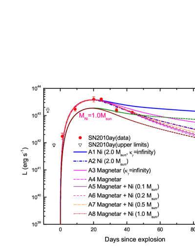
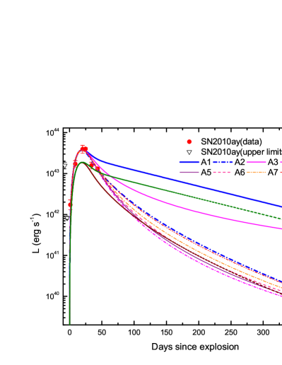
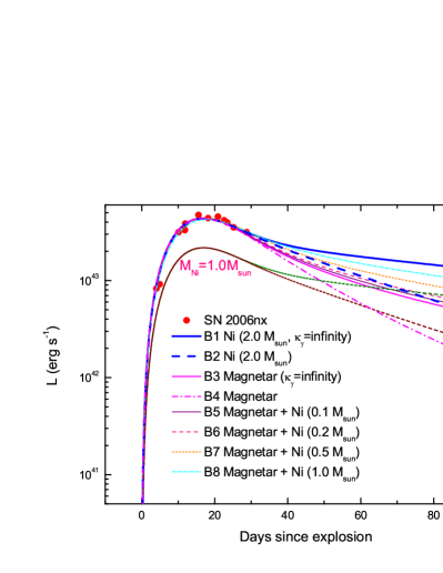
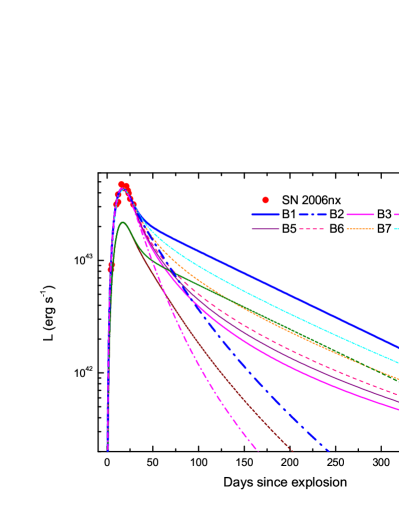
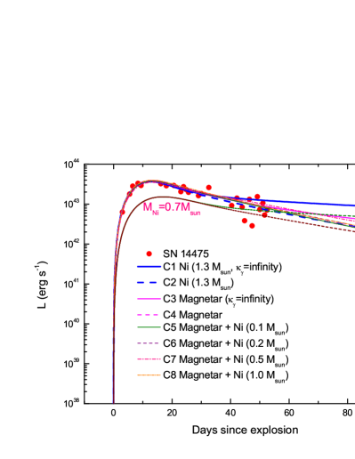
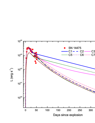
Figure 1: Model fits using the ⁵⁶Ni-decay models, the magnetar models as well as the hybrid (⁵⁶Ni-decay + magnetar) models for SN 2010ay ($top$), SN 2006nx ($middle$), and SN 14475 ($bottom$). Left panels: -10$-$100 days after the explosion; Right panels: -10$-$400 days after the explosion. Data and upper limits of SN 2010ay are obtained from Sanders et al. (2012), data of SN 2006nx and SN 14475 are obtained from Taddia et al. (2015). The horizontal axis represents the time since the explosion in the rest frame. Parameters for Models A1-A8, B1-B8, and C1-C8 are shown in Table 1. $\kappa$ = 0.07 cm² g^-1 is adopted. In all panels, we add two light curves reproduced by the ⁵⁶Ni-decay models with 1 $M_{\odot}$ and 0.7 $M_{\odot}$, without and with $\gamma$-ray leakage. It can be seen from these light curves that 1 $M_{\odot}$ or 0.7 $M_{\odot}$ of ⁵⁶Ni is inadequate to power these SNe.

The parameters for the ⁵⁶Ni-powered model are listed in Table 1 and the light curves reproduced by these sets of parameters are shown in Fig. 1 (Models A1 and A2 for SN 2010ay, B1 and B2 for SN 2006nx, C1 and C2 for SN 14475).

Using the empirical relation between the peak absolute magnitude and the mass of ⁵⁶Ni derived by Drout et al. (2011), Sanders et al. (2012) inferred that the ⁵⁶Ni mass of SN 2010ay is $~{}0.9_{-0.1}^{+0.1}~{}M_{\odot}$. However, it can be seen from Fig. 1 and Table 1 that $1.0~{}M_{\odot}$ of ⁵⁶Ni is inadequate to power the peak luminosity of SN 2010ay solely. To power the peak luminosity, $\sim 2.0~{}M_{\odot}$ of ⁵⁶Ni must be required. The value $2.0~{}M_{\odot}$ is consistent with the value $1.81^{+0.21}_{-0.21}~{}M_{\odot}$ derived by the Arnett law.

It can be seen from Fig. 1 and Table 1 that $2.0~{}M_{\odot}$ and $1.3~{}M_{\odot}$ of ⁵⁶Ni are required to power the peak luminosities of SN 2006nx and SN 14475, respectively. The values $2.0~{}M_{\odot}$ and $1.3~{}M_{\odot}$ are consistent with the value $1.86^{+0.12}_{-0.12}~{}M_{\odot}$ and $1.27^{+0.08}_{-0.09}~{}M_{\odot}$ derived by Taddia et al. (2015) as well as the values $2.08^{+0.24}_{-0.24}~{}M_{\odot}$ and $1.63^{+0.19}_{-0.19}~{}M_{\odot}$ derived by the Arnett law.

In this paper, we adopt a fiducial value of optical opacity 0.07 cm² g^-1. In many other papers, however, the fiducial values of opacity have also been assumed to be 0.06 cm² g^-1 (e.g., Valenti et al., 2011; Lyman et al., 2014), 0.08 cm² g^-1 (e.g., Arnett, 1982; Mazzali et al., 2000), 0.10 cm² g^-1 (e.g., Nugent et al., 2011; Inserra et al., 2013; Wheeler et al., 2014) and 0.2 cm² g^-1 (e.g., Kasen & Bildsten, 2010; Nicholl et al., 2014). It is necessary to point out that more ⁵⁶Ni for the ⁵⁶Ni model or smaller $P_{0}$ of the magnetar for the magnetar model is required to account for the peak luminosity of SN 2010ay, SN 2006nx, and SN 14475 when $\kappa$ is larger than 0.07 cm² g^-1 since larger $\kappa$ results in larger diffusion time and lower the peak luminosities. On the other hand, when $\kappa$ is smaller than 0.07 cm² g^-1, less ⁵⁶Ni or larger $P_{0}$ are required for the same peak luminosity. For example, If we assume that SN 2010ay is powered by ⁵⁶Ni and $\kappa=$ 0.06 cm² g^-1, then $\sim 1.8~{}M_{\odot}$ of ⁵⁶Ni must be synthesized, which is smaller than $2.0~{}M_{\odot}$ when $\kappa=$ 0.07 cm² g^-1.

To maintain the same peak luminosities and shapes of light curves, $\kappa M_{\rm ej}/v$ must be invariant. Because the photospheric velocities of SN 2010ay, SN 2006nx, and SN 14475 are fixed, so $\kappa M_{\rm ej}=$constant is required. Hence, smaller $\kappa$ requires larger $M_{\rm ej}$, as illustrated in Fig. 2.

3.2 The upper limits of ⁵⁶Ni mass

A consensus has been reached that iron$-$core-collapse SNe can synthesize a large amount of ⁵⁶Ni. However, could these 3 SN explosions produce $\sim 1.3~{}M_{\odot}$ or $\sim 2.0~{}M_{\odot}$ of ⁵⁶Ni? To get reasonable upper limits for the ⁵⁶Ni masses synthesized in the explosions of SN 2010ay, SN 2006nx, and SN 14475, we perform semi-quantitative estimates.

The radius of the ⁵⁶Ni layer can be given as

$$R_{\rm Ni} = \left(\frac{E_{\rm exp}+E_{\rm bin}}{\frac{4}{3}{\pi}aT^{4}}\right)^{1/3}$$ (8)

$$\simeq 4.0\times 10^{3}\left(\frac{E_{\rm exp}+E_{\rm bin}}{10^{51}{\rm\;erg}}\right)^{1/3}\left(\frac{T}{5\times 10^{9}{\rm\;K}}\right)^{-4/3}~{}\mbox{km}$$

where $E_{\rm exp}$, $E_{\rm bin}$ are the explosion energy and the binding energy of the progenitor, respectively, $T$ is the temperature of the ejecta, $a~{}=~{}7.56566\times 10^{15}$ erg cm^-3 K^-4 is the radiation energy density constant. Since $M_{\rm Ni}~{}={4/3}\rho_{\rm Ni}{\pi}R_{\rm Ni}^{3}$, $M_{\rm Ni}$ is therefore approximately proportional to ${E_{\rm exp}+E_{\rm bin}}\simeq{E_{\rm exp}}$ which in turn is approximately proportional to the kinetic energy $E_{\rm K}$, see, e.g., the bottom panel of Fig. 7 of Hamuy (2003) and the left panel of Fig. 23 of Pejcha & Thompson (2014). The masses of the progenitors also influence the yields of ⁵⁶Ni. These facts can also be seen in Fig. 7 and Table 3 in Umeda & Nomoto (2008). The typical masses of the ⁵⁶Ni synthesized during the explosive silicon burning are $\sim 0.1-0.5M_{\odot}$ for CCSNe.

We compare SN 2010ay, SN 2006nx, and SN 14475 with the prototype hypernova SN 1998bw. The kinetic energy of SN 2010ay ($\approx 1.1\times 10^{52}$ erg, Sanders et al., 2012) and SN 14475 ($\approx 4.71^{+12.29}_{-2.41}\times 10^{51}$ erg, Taddia et al., 2015) are about a factor of 3-5 smaller than that of SN 1998bw ($\approx 3-5\times 10^{52}$ erg, Iwamoto et al., 1998; Nakamura et al., 2001; Lyman et al., 2014), so we can infer that their ⁵⁶Ni yields must be $\lesssim 0.5~{}M_{\odot}$ and $\sim 0.1-0.2~{}M_{\odot}$ which are significantly smaller than $1~{}M_{\odot}$ . The kinetic energy of SN 2006nx ($\approx 2.160^{+3.753}_{-0.501}\times 10^{52}$ erg, Taddia et al., 2015) has rather significant uncertainty, but its upper limit ($\approx 5.91\times 10^{52}$ erg) is slightly larger than that of SN 1998bw ($\approx 5\times 10^{52}$ erg). Hence, the ⁵⁶Ni yield of SN 2006nx must be $\sim 0.5~{}M_{\odot}$ and smaller than $1~{}M_{\odot}$.

We can constrain the ⁵⁶Ni masses of SN 2010ay, SN 2006nx, and SN 14475 using another method. Umeda & Nomoto (2008) calculated the mass of the synthesized ⁵⁶Ni in CCSNe with progenitor Zero-Age Main-Sequence masses $M_{\rm ZAMS}\leq 100M_{\odot}$ and found that the typical ⁵⁶Ni mass is at most 20% of the ejecta mass. According to our light-curve modeling, the ejecta mass of SN 2010ay, SN 2006nx, and SN 14475 to be 6.5 $M_{\odot}$, 3.6 $M_{\odot}$, and 2.1  $M_{\odot}$, respectively, see Table 1. Combining these two results, $\lesssim$ 1.3, 0.7, and 0.4 $M_{\odot}$ of ⁵⁶Ni can be synthesized in the explosions, respectively. If the masses of ⁵⁶Ni are $\sim$ 2.0, 2.0, and 1.3 $M_{\odot}$, the values of $M_{\rm Ni}/M_{\rm ej}$ are $\sim$ 0.31, 0.56, and 0.62 (see Table 1) which (far) exceed the upper limit ($\sim 0.2$) of the mass ratio given by Umeda & Nomoto (2008) for CCSNe.

These results indicate that the ⁵⁶Ni-decay model cannot account for the light curves of SN 2010ay, SN 2006nx, and SN 14475 and these three SNe are probably solely or partly powered by other energy sources.

3.3 The magnetar spin-down energy model

Encountered by the above difficulty, alternative energy-reservoir models must be seriously considered. According to their inferred ratio of $M_{\rm Ni}$ to $M_{\rm ej}$, $\sim 0.2$, Sanders et al. (2012) suggested that SN ejecta-circumstellar medium interaction could also contribute to the high peak luminosity of SN 2010ay as well, yet they did not perform further investigation for this possibility. Owing to the lack of narrow and/or intermediate-width emission lines indicative of interactions between the SN ejecta and hydrogen- and helium-deficient CSM, we argue that ejecta-CSM interactions could hardly provide a reasonable interpretation for the excess luminosities of SN 2010ay, SN 2006nx, and SN 14475. Hence we attribute the luminosity excess instead to energy injection by the nascent magnetars and employ the magnetar model to explain the data for these SNe Ic.

The parameters for the magnetar model are listed in Table 1 and the light curves reproduced by the sets of parameters are shown in Fig. 1 (Models A3 and A4 for SN 2010ay, B3 and B4 for SN 2006nx, C3 and C4 for SN 14475). It can be seen from Fig. 1 that the magnetar model can well fit the data. These results indicate that this model can be responsible for the light curves of SN 2010ay, SN 2006nx, and SN 14475, i.e., SN 2010ay, SN 2006nx, and SN 14475 are probably powered by nascent millisecond (or $\sim$ 10 ms) magnetars.

3.4 The hybrid (⁵⁶Ni + magnetar) model

When the ejecta masses of CCSNe are not very large, e.g., $\lesssim 2~{}M_{\odot}$, the ⁵⁶Ni synthesized are generally $\lesssim 0.1~{}M_{\odot}$, which contribute a minor fraction of the luminosity of luminous SNe and can be neglected in the fit. Inserra et al. (2013) demonstrated that the magnetar models without ⁵⁶Ni and with $\sim 0.1~{}M_{\odot}$ of ⁵⁶Ni are similar and therefore neglected the contribution from ⁵⁶Ni for their six SLSNe Ic.

However, SN 2010ay, SN 2006nx, and SN 14475 are not SLSNe and their ejected ⁵⁶Ni might have a mass of $\sim 0.1-0.5M_{\odot}$, so the contribution from ⁵⁶Ni must be taken into account in our modeling.

Since the exact values of $M_{\rm Ni}$ of these three SNe are unknown when the contribution from magnetars is considered, we plot light curves corresponding to a variety of masses of ⁵⁶Ni. The typical values of $M_{\rm Ni}$ adopted here are 0.1, 0.2, 0.5 and 1.0 $M_{\odot}$ . The parameters for the hybrid (⁵⁶Ni + magnetar) model are also listed in Table 1 and a family of light curves reproduced by these sets of parameters are shown in Fig. 1 (Models A5$-$A8 for SN 2010ay, B5$-$B8 for SN 2006nx, C5$-$C8 for SN 14475).

The ⁵⁶Ni mass with $\lesssim 0.5~{}M_{\odot}$, the energy released by the rapidly spinning magnetar is still the dominant energy source in powering the optical light curves of SN 2010ay, SN 2006nx, and SN 14475. When the ⁵⁶Ni mass is $\sim 1~{}M_{\odot}$, the energy released by ⁵⁶Ni is comparable with or exceed the energy released by the magnetar. If the ⁵⁶Ni masses are $\lesssim 1~{}M_{\odot}$ and the magnetar parameters are adjusted, the light curves reproduced by the hybrid model are all in good agreement with observations, indicating that $\lesssim 1~{}M_{\odot}$ of ⁵⁶Ni is admitted to be synthesized in their explosions.

On the other hand, there are rather significant discrepancies in the late-time ($\gtrsim 50$ days) light curves reproduced by different masses of ⁵⁶Ni. These discrepancies cannot be eliminated by adjusting the magnetar parameters since the decline rate of late-time light curves is determined mainly by ⁵⁶Co decay rate and the value of $\kappa_{\gamma}$.

We cannot determine the precise masses of ⁵⁶Ni synthesized in the explosions of these SNe, because there is no precise late-time observation. Provided that there are some late-time data observed, it would be powerful enough to constrain the precise value of their ⁵⁶Ni mass.

To compare these models, we calculate the values of $\chi^{2}$/d.o.f for all these theoretical light curves , see Table 1. Since the ⁵⁶Ni-powered models are disfavored in explaining these three SNe, as discussed above, we do not discuss them here even if they give smaller $\chi^{2}$/d.o.f.. Therefore, we only consider the magnetar-powered models and hybrid models. It can be seen from the last column in Table 1 that Models A4 (magnetar-powered model with hard emission leakage), B7 (magnetar and 0.5 $M_{\odot}$ of ⁵⁶Ni), and C5 (magnetar and 0.1 $M_{\odot}$ of ⁵⁶Ni) have the smallest $\chi^{2}$/d.o.f. Nevertheless, due to the absence of late-time data, we still cannot conclude that these models are most favorable ones.

3.5 An analysis for the origin of the kinetic energy

It is necessary to take into account the kinetic energy coming from the $P$d$V$ work. The tapped rotational energy of a nascent magnetar ($E_{\rm NS}\simeq 2\times 10^{52}\left({P_{0}}/{1~{}{\rm ms}}\right)^{-2}$ erg) must be split into radiation energy ($E_{\rm rad}$) and kinetic energy ($E_{\rm K,mag}$). The former heat the ejecta, while the latter accelerate the ejecta. When $P_{0}\sim 9$ ms, $E_{\rm NS}\simeq 3.0~{}\times 10^{50}~{}{\rm erg}$. Even if all of the rotational energy of the putative magnetar is converted into kinetic energy of the ejecta , $E_{\rm K,mag}\approx E_{\rm NS}\simeq 3.0~{}\times 10^{50}~{}{\rm erg}$, it is still far less than the total kinetic energy ($E_{\rm K}\gtrsim 5\times 10^{51}$ erg) of SN 2010ay, SN 2006nx, as well SN 14475 and can therefore be completely neglected.

We now turn our attention to the neutrino-driven mechanism (Bethe & Wilson, 1985). Hydrodynamic supernova simulations suggest that the neutrino-driven mechanism can produce SN energies $\lesssim 2\times 10^{51}$ erg (Ugliano et al., 2012), far less than the observed kinetic energy of $E_{\rm K}\gtrsim 5\times 10^{51}$ erg, indicating that there must be another mechanism accounting for the additional energy of $\gtrsim 3\times 10^{51}$ erg. A popular scenario to explain energetic SNe with kinetic energies $\gtrsim 10^{52}$ erg is the “collapsar” model involving a “BH-disk” system, in which the “BH-disk” system generates bipolar jet/outflow while the “disk wind” ensures that the progenitor star explodes and synthesizes enough amount of ⁵⁶Ni. However, our fittings have demonstrated that the newly formed magnetar did not collapse to a black hole at least several days after the explosion. Hence, the huge kinetic energy might stem from some magnetohydrodynamic processes (e.g., magnetic buoyancy, magnetic pressure, hoop stresses, etc) related to the proto-NS themselves (Wheeler et al., 2000) after which the magnetars inject their rotational energy to heat the ejecta and generate the light curves.

4 Discussion and Conclusions

Most type Ic CCSNe produce ⁵⁶Ni which release energy to the ejecta via cascade decay and central NSs which convert a portion of their rotational energy into heating energy of the ejecta via the magnetic dipole radiation. For almost all normal CCSNe, $\sim$ 0.1$-$0.7 $M_{\odot}$ of ⁵⁶Ni are adequate to power the peak and post-peak decline of observational light curves and the contribution of NSs can be neglected . In contrast, for SLSNe Ic which are lack of evidence of interaction and cannot be explained by ⁵⁶Ni solely, millisecond NSs (magnetars) can supply almost all input power and the contribution of ⁵⁶Ni can be neglected.

For luminous SNe Ic with $-19.5\gtrsim M_{\rm peak}\gtrsim-21$ mag in any band, however, both contributions from ⁵⁶Ni and NSs cannot be neglected without detailed modeling since the ⁵⁶Ni permitted by completely explosive burning are usually inadequate to power the high peak luminosities while the production of $\sim 0.1-\sim 0.5M_{\odot}$ of ⁵⁶Ni is reasonable and may contribute a significant portion of the total luminosity. Therefore, these “gap-filler” events which bridge normal SNe and SLSNe must be explained by a unified model which contain contributions from ⁵⁶Ni and NSs.

To illustrate the necessity of constructing the unified model, we select and apply this model to three luminous SNe Ic-BL, SN 2010ay, SN 2006nx, and SN 14475. We tested the possibility that the luminosity evolutions of SN 2010ay, SN 2006nx, and SN 14475 are solely governed by radioactive ⁵⁶Ni cascade decay using the semi-analytical method and demonstrated that too large amounts, roughly 2.0, 2.0, and 1.3 $M_{\odot}$ of ⁵⁶Ni, are needed to power their peak luminosities, respectively. These results disfavor the ⁵⁶Ni model in explaining the light curves of SN 2010ay, SN 2006nx, and SN 14475, since the ratios of $M_{\rm Ni}$ to $M_{\rm ej}$ are 0.31, 0.56, and 0.62, respectively, significantly exceeding the upper limit ($\sim 0.2$) calculated for CCSNe (Umeda & Nomoto, 2008).

Then we alternatively invoke the magnetar model to reproduce the light curves of SN 2010ay, SN 2006nx, and SN 14475 and show that the light curves reproduced can be well consistent with the observations, suggesting that SN 2010ay, SN 2006nx, and SN 14475 are probably powered by spin-down energy injection from newly born millisecond magnetars. It seems that the magnetar model can account for the light curves of these SNe and ⁵⁶Ni is not necessary to be introduced. However, a moderate amount of ⁵⁶Ni, $\sim 0.1-0.5M_{\odot}$, can be expected in completely explosive burning of silicon shell and could give rather energy to those not very luminous SNe. So ⁵⁶Ni cannot be neglected when the SNe are not very luminous. Thus we use the hybrid model to fit these three SNe.

We set $M_{\rm Ni}$ = 0.1, 0.2, 0.5 and 1.0 $M_{\odot}$ and find that $\lesssim 0.2~{}M_{\odot}$ of ⁵⁶Ni can not significantly influence the theoretical light curves while $\gtrsim 0.5~{}M_{\odot}$ of ⁵⁶Ni can effectively alters the shapes of the light curves, leading us to adjust the magnetar parameters to fit the observations. Therefore, all these models (⁵⁶Ni, magnetar, and hybrid), with different amount of ⁵⁶Ni (from 0 to 2 or 1.3 $M_{\odot}$), fit the light curves equally well and can be unified into a unified model. Among these models, the ⁵⁶Ni model needs huge, unrealistic amounts of ⁵⁶Ni, resulting in over-high ratios of $M_{\rm Ni}$ to $M_{\rm ej}$. In contrast, the magnetar model needs no ⁵⁶Ni and conflict with the basic theory of nuclear synthesis. The hybrid model is reasonable in explaining these luminous SNe.

These facts suggest that these three luminous SNe Ic are all powered by both ⁵⁶Ni and magnetars, indicating that the magnetars contribute a large fraction of but not all power in driving their light curves. So we can conclude that, when $M_{\rm peak}$ (in any band) is $\lesssim-21$ mag, the contribution of ⁵⁶Ni can be neglected in light-curve modeling; when $-21\lesssim M_{\rm peak}\lesssim-19.5$ mag, the contribution from the magnetar cannot be omitted in modeling while the contribution from ⁵⁶Ni must be considered seriously; but when $M_{\rm peak}\gtrsim-19.5$ mag, the contribution of the magnetar can generally be neglected (but see Maeda et al., 2007).

It should be pointed out that the “fiducial cutoffs” $-19.5$ mag and $-21$ mag that divide the normal SNe, luminous SNe and SLSNe are artificially given and do not have unambiguous physical meanings. Although no consistent picture of these SNe Ic with rather different peak luminosities has emerged so far, it seems that they have similar physical nature and similar power sources, e.g., ⁵⁶Ni and newly born NSs (magnetars), while the former result in a relative narrow range of peak-luminosities owing to the existence of the upper limit of ⁵⁶Ni yields and thus the peak luminosities, the latter might produce a wide range of peak-luminosities since the period of newly born NSs can vary from several milliseconds to several seconds, and magnetic field strength of them can be up to $10^{15}$ G. These two power sources could result in a continuous sequence of peak-luminosities, covering normal, luminous, and very luminous SNe Ic and unifying most of them into a whole category in which normal SNe are powered by slow-spinning NSs and ⁵⁶Ni, while luminous SNe and SLSNe are mainly powered by fast-spinning (millisecond) magnetar and ⁵⁶Ni. The similarity between late-time spectra of SLSNe Ic and spectra of normal SNe Ic-BL (Pastorello et al., 2010; Gal-Yam, 2012; Inserra et al., 2013) also supports this unified picture.

Furthermore, we suggest that many SNe Ic with $M_{\rm peak}\lesssim-19.5$ mag might be partly powered by a nascent magnetar, i.e., the very young SN remnants of the explosions may harbor magnetars. The discrepancy in brightness between luminous SNe Ic and SLSNe Ic stem mainly from the initial spin periods of the magnetars, the former have $P_{0}~{}\sim 7-15$ ms, while the latter have $P_{0}~{}\sim 1-6$ ms (Inserra et al., 2013; Nicholl et al., 2014). For luminous SNe Ic, power from magnetars with $P_{0}~{}\sim 10$ ms can become comparable to or exceed that from ⁵⁶Ni, and vice versa; for SLSNe Ic, millisecond magnetars usually overwhelm ⁵⁶Ni in powering them.

For the sake of completeness, both these two power sources must be taken into account in light-curve modeling. Nevertheless, we still emphasize that this unified scenario is especially important for the gap-filler SNe Ic since they, as aforementioned, are hardly powered solely by ⁵⁶Ni but ⁵⁶Ni can contribute a non-negligible portion of the luminosity and must be considered in modeling. Modeling for these luminous SNe can also help us to understand how normal SNe Ic relate to SLSNe Ic. Besides, even if a SN or superluminous SN that can be solely explained by the magnetar model, Fe line in its spectrum, if observed, must be explained by introducing a moderate amount of ⁵⁶Ni, because the magnetar model cannot explain Fe line (Kasen & Bildsten, 2010). This is another advantage of the unified model. In the recent excellent review for SLSNe, Gal-Yam (2012) already noticed these “gap-filler” SNe and reckoned that they are likely to be intermediate events between radioactivity-powered SNe/SLSNe Ic and the SLSNe Ic powered by some other processes. Our analysis has confirmed this conjecture and furthermore demonstrated that these “intermediate events” are likely to have the same power sources and the difference between them and their lower-luminosity and higher-luminosity cousins are mainly due to the physical properties of the nascent neutron stars embedded in their debris.

While this unified energy-reservoir model seems reasonable for SN 2010ay, SN 2006nx, and SN 14475, the precise value of ⁵⁶Ni yields cannot be determined, indicating that the traditional method that suppose all power given by ⁵⁶Ni cascade decay is not always reliable in inferring the ⁵⁶Ni yields of CCSNe, especially for those luminous and very luminous ones. To discriminate these models and roughly determine the ⁵⁶Ni mass as well as the parameters of the putative NSs, late-time ($\gtrsim 100-200$ d) data are required. Unfortunately, these three SNe are all lacking late-time observations, especially for SN 14475 whose luminosity measurements in the period between 25 and 35 days after the peak are rather uncertain.

Spectral analysis would be of outstanding importance in determining the precise values of ⁵⁶Ni and $M_{\rm ej}$ as well as the parameters of the NS parameters. In practice, detection and analysis of nebular emission from ⁵⁶Fe resulted from the ⁵⁶Ni cascade decay and other heavy elements are necessary for precise measurement of ⁵⁶Ni yields. The ejecta mass $M_{\rm ej}$ can significantly influence the rise time, shape, and peak luminosity as well as the ratio of $M_{\rm Ni}$ to $M_{\rm ej}$ of a SN, so it is also a very important quantity in modeling. Due to the uncertainty of optical opacity $\kappa$, $M_{\rm ej}$ cannot be precisely determined using solely the light-curve modeling (see Fig.2). To get more precise value of the ejecta mass or at least a rigorous upper/lower limit, as performed by Gal-Yam et al. (2009) for SN 2007bi, nebular modeling are required.

The above procedures need very precise observations and spectral analysis lasting several hundred days after the detection of the first light. Unfortunately, no late-time photometric data and spectra have been observed for these three SNe, especially for SN 2006nx and SN 14475. We cannot get enough information to determine the precise masses of ⁵⁶Ni and the real values of magnetar parameters. Hence, we cannot distinguish among these model parameters and therefore to have a more precise scenario. We can expect that future high cadence multi-epoch UV$-$optical$-$NIR observations of the luminous SNe can pose stringent constraints on the parameters of the nascent NSs and ⁵⁶Ni yields.

Table 1: Parameters for unified (⁵⁶Ni-decay, magnetar spin-down, and hybrid (⁵⁶Ni + magnetar)) modeling

	$M_{\rm ej}$	$B$	$P$	$v$	$\kappa$	$\kappa_{\gamma}$	$M_{\rm Ni}$	$M_{\rm Ni}/M_{\rm ej}$	$\chi^{2}$/d.o.f
	($M_{\odot}$)	($10^{14}$ G)	(ms)	($c$)	(cm2 g-1)	(cm2 g-1)	($M_{\odot}$)
SN 2010ay
Model A1 a	6.5	0	$\infty$	0.064	0.07	$\infty$	2.0	0.308	5.41
Model A2 a	6.5	0	$\infty$	0.064	0.07	$0.014$	2.0	0.308	1.05
Model A3 b	6.5	4.5	8.8	0.064	0.07	$\infty$	0	0	2.36
Model A4 b	6.5	4.5	8.8	0.064	0.07	$0.021$	0	0	1.34
Model A5 c	6.5	4.5	9.0	0.064	0.07	$0.021$	0.1	0.015	2.00
Model A6 c	6.5	4.5	9.3	0.064	0.07	$0.021$	0.2	0.031	2.05
Model A7 c	6.5	5.2	10.3	0.064	0.07	$0.021$	0.5	0.077	2.11
Model A8 c	6.5	7.2	12.5	0.064	0.07	$0.021$	1.0	0.154	2.12
SN 2006nx
Model B1 a	3.6	0	$\infty$	0.051	0.07	$\infty$	2.0	0.556	1.24
Model B2 a	3.6	0	$\infty$	0.051	0.07	$0.037$	2.0	0.556	1.22
Model B3 b	3.6	4.5	8.8	0.051	0.07	$\infty$	0	0	1.58
Model B4 b	3.6	4.5	8.8	0.051	0.07	$0.037$	0	0	1.56
Model B5 c	3.6	4.5	9.0	0.051	0.07	$\infty$	0.1	0.028	1.60
Model B6 c	3.6	4.5	9.2	0.051	0.07	$\infty$	0.2	0.056	1.44
Model B7 c	3.6	4.5	9.8	0.051	0.07	$\infty$	0.5	0.139	1.11
Model B8 c	3.6	4.8	11.9	0.051	0.07	$\infty$	1.0	0.278	1.60
SN 14475
Model C1 a	2.1	0	$\infty$	0.062	0.07	$\infty$	1.3	0.619	4.10
Model C2 a	2.1	0	$\infty$	0.062	0.07	$0.063$	1.3	0.619	2.78
Model C3 b	2.1	4.8	10.4	0.062	0.07	$\infty$	0	0	3.03
Model C4 b	2.1	4.8	10.4	0.062	0.07	$0.133$	0	0	3.30
Model C5 c	2.1	4.8	10.7	0.062	0.07	$0.133$	0.1	0.048	2.97
Model C6 c	2.1	4.8	10.9	0.062	0.07	$0.133$	0.2	0.095	3.53
Model C7 c	2.1	4.8	12.6	0.062	0.07	$0.133$	0.5	0.238	3.54
Model C8 c	2.1	4.8	15.2	0.062	0.07	$0.063$	1.0	0.476	4.03

^a The ⁵⁶Ni-decay model.
^b The magnetar model.
^c The hybrid (⁵⁶Ni + magnetar) model.

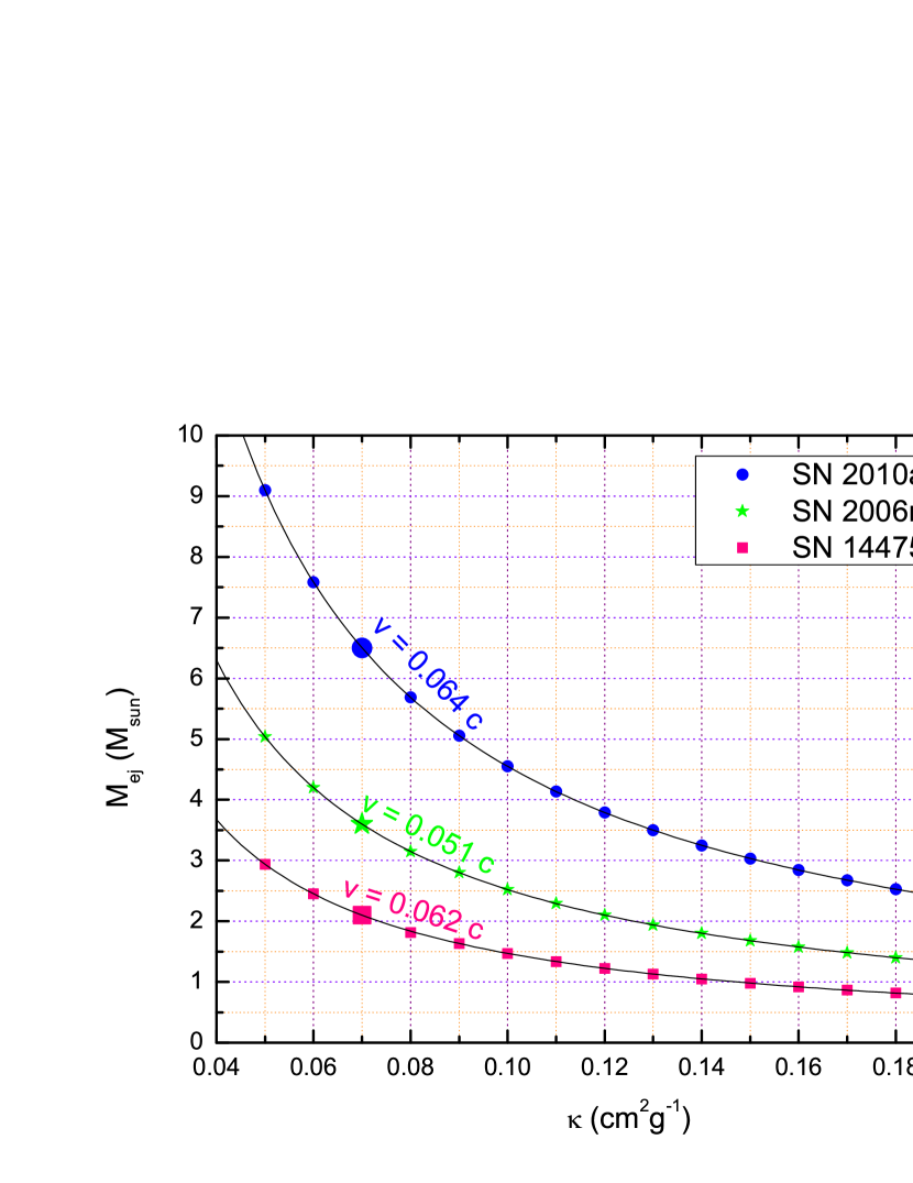
Figure 2: The values of $\kappa$ vs. the values of $M_{\rm ej}$ for SN 2010ay, SN 2006nx, and SN 14475. The values of $\kappa$ vary from 0.05 cm² g^-1 to 0.20 cm² g^-1, resulting in rather different values of $M_{\rm ej}$ required. Big Circle, Star, and Square correspond to SN 2010ay, SN 2006nx, and SN 14475 with $\kappa=0.07$ cm² g^-1, respectively.

References

- Arnett (1979) Arnett, W. D. 1979, ApJL, 230, L37
- Arnett (1982) Arnett, W. D. 1982, ApJ, 253, 785
- Ben-Ami et al. (2014) Ben-Ami, S., Gal-Yam, A., Mazzali, P. A., et al. 2014, ApJ, 785, 37
- Bethe & Wilson (1985) Bethe, H. A., & Wilson, J. R. 1985, ApJ, 295, 14
- Bucciantini et al. (2008) Bucciantini, N., Quataert, E., Arons, J., Metzger, B. D., & Thompson, T. A. 2008, MNRAS, 383, L25
- Cano et al. (2014) Cano, Z., de Ugarte Postigo, A., Pozanenko, A., et al. 2014, A&A, 568, 19
- Cappellaro et al. (1997) Cappellaro, E., Mazzali, P. A., Benetti, S., et al. 1997, A&A, 328, 203
- Candia et al. (2003) Candia, P., Krisciunas, K., Suntzeff, N. B., et al. 2003, PASP, 115, 277
- Chatzopoulos et al. (2009) Chatzopoulos, E., Wheeler, J. C., & Vinko, J. 2009, ApJ, 704, 1251
- Chatzopoulos et al. (2012) Chatzopoulos, E., Wheeler, J. C., & Vinko, J. 2012, ApJ, 746, 121
- Chatzopoulos et al. (2013) Chatzopoulos, E., Wheeler, J. C., Vinko, J., Horvath, Z. L., & Nagy, A. 2013, ApJ, 773, 76
- Chevalier (1982) Chevalier, R. A. 1982, ApJ, 258, 790
- Chevalier & Fransson (1994) Chevalier, R. A., & Fransson, C. 1994, ApJ, 420, 268
- Chevalier & Irwin (2011) Chevalier, R. A., & Irwin, C. M. 2011, ApJL, 729, L6
- Chugai (1994) Chugai, N. N. 1994, MNRAS, 326, 1448
- Clocchiatti & Wheeler (1997) Clocchiatti, A., & Wheeler, J. C. 1997, ApJ, 491, 375
- Contardo et al. (2000) Contardo, G., Leibundgut, B., & Vacca, W. D. 2000, A&A, 359, 876
- Colgate & McKee (1969) Colgate, S. A., & McKee, C. 1969, ApJ, 157, 623
- Colgate et al. (1980) Colgate, S. A., Petschek, A. G., & Kriese, J. T. 1980, ApJL, 237, L81
- Dai & Lu (1998a) Dai, Z. G., & Lu, T. 1998a, A&A, 333, L87
- Dai & Lu (1998b) Dai, Z. G., & Lu, T. 1998b, PhRvL, 81, 4301
- Dai (2004) Dai, Z. G. 2004, ApJ, 606, 1000
- Dai & Liu (2012) Dai, Z. G., & Liu, R. Y. 2012, ApJ, 759, 58
- Drake et al. (2009) Drake, A. J., Djorgovski, S. G., Mahabal, A., et al. 2009, ApJ, 696, 870
- Drout et al. (2011) Drout, M. R., Soderberg, A. M., Gal-Yam, A., et al. 2011, ApJ, 741, 97
- Drout et al. (2013) Drout, M. R. , Soderberg, A. M., Mazzali P. A., et al. 2013, ApJ, 774, 58
- Falk & Arnett (1977) Falk, S. W., & Arnett, W. D. 1977, ApJS, 33, 515
- Filippenko (1997) Filippenko, A. V. 1997, ARA&A, 35, 309
- Gal-Yam et al. (2009) Gal-Yam, A., Mazzali, P., Ofek, E. O., et al. 2009, Natur, 462, 624
- Gal-Yam (2012) Gal-Yam, A. 2012, Science, 337, 927
- Ginzburg & Balberg (2012) Ginzburg, S., & Balberg, S. 2012, ApJ, 757, 178
- Hamuy (2003) Hamuy, M. 2003, ApJ, 582, 905
- Heger & Woosley (2002) Heger, A., & Woosley, S. E. 2002, ApJ, 567, 532
- Hjorth & Bloom (2012) Hjorth, J., & Bloom, J. S., 2012, in Chapter 9 in Gamma-Ray Bursts, ed. C. Kouveliotou, R. A. M. J. Wijers, & S. Woosley (Cambridge Astrophysics Series, Vol. 51; Cambridge: Cambridge Univ. Press), 169
- Howell et al. (2013) Howell, D. A., Kasen, D., Lidman, C., et al. 2013, ApJ, 779, 98
- Inserra et al. (2013) Inserra, C., Smartt, S. J., Jerkstrand, A., et al. 2013, ApJ, 770, 128
- Iwamoto et al. (1998) Iwamoto, K., Mazzali, P. A., Nomoto, K., et al. 1998, Natur, 395, 672
- Janka et al. (2007) Janka, H.-T., Langanke, K., Marek, A., Martinez-Pinedo, G., & Müller, B. 2007, Physics Reports, 442, 1-6, 38
- Kasen & Woosley (2009) Kasen, D., & Woosley, S. E. 2009, ApJ, 703, 2205
- Kasen & Bildsten (2010) Kasen, D., & Bildsten, L. 2010, ApJ, 717, 245
- Klein & Chevalier (1978) Klein, R. I., & Chevalier, R. A. 1978, ApJL, 223, L109
- Kotera et al. (2013) Kotera, K., Phinney, E. S., & Olinto, A. V. 2013, MNRAS, 432, 3228
- Lundqvist et al. (2001) Lundqvist, P., Kozma, C., Sollerman, J., & Fransson, C. 2001, A&A, 374, 629
- Lyman et al. (2014) Lyman, J. D., Bersier, D., James, P. A., Mazzali, P. A., Eldridge, J., Fraser, M., & Pian, E. 2014, arXiv:1406.3667
- MacFadyen & Woosley (1999) MacFadyen, A. I., & Woosley, S. E. 1999, ApJ, 524, 262
- Maeda et al. (2003) Maeda, K., Mazzali, P. A., Deng, J., Nomoto, K., Yoshii, Y., Tomita, H., & Kobayashi, Y. 2003, ApJ, 593, 931
- Maeda et al. (2007) Maeda, K., Tanaka, M., Nomoto, K., Tominaga, N., Kawabata, K., Mazzali, P. A., Umeda, H., Suzuki, T., & Hattori, T. 2007, ApJ, 666, 1069
- Mazzali et al. (2000) Mazzali, P. A., Iwamoto, K., & Nomoto, K. 2000, ApJ, 545, 407
- Mazzali et al. (2006) Mazzali, P. A., Deng, J., Pian, E., et al. 2006, ApJ, 645, 1323
- McCrum et al. (2014) McCrum, M., Smartt, S. J., Kotak, R., et al. 2014, MNRAS, 437, 656
- Metzger et al. (2007) Metzger, B. D., Thompson, T. A., & Quataert, E. 2007, ApJ, 659, 561
- Metzger et al. (2011) Metzger, B. D., Giannios, D., Thompson, T. A., Bucciantini, N., & Quataert, E. 2011, MNRAS, 413, 2031
- Moriya et al. (2013) Moriya, T. J., Blinnikov, S. I., Tominaga, N., Yoshida, N., Tanaka, M., Maeda, K., & Nomoto, K. 2013, MNRAS, 428, 1020
- Nakamura et al. (2001) Nakamura, T., Mazzali, P. A., Nomoto, K., & Iwamoto, K. 2001, ApJ, 550, 991
- Nicholl et al. (2013) Nicholl, M., Smartt, S. J., Jerkstrand, A., et al. 2013, Natur, 502, 346
- Nicholl et al. (2014) Nicholl, M., Jerkstrand, A., Inserra, C., et al. 2014, MNRAS, 444, 2096
- Nugent et al. (2011) Nugent, P. E., Sullivan, M., Cenko, S. B., et al. 2011, Natur, 480, 344
- Ofek et al. (2013) Ofek, E. O., Sullivan, M., Cenko, S. B., et al. 2013, Natur, 494, 65
- Ostriker & Gunn (1971) Ostriker, J. P., & Gunn, J. E. 1971, ApJL, 164, L95
- Pastorello et al. (2010) Pastorello, A., Smartt, S. J., Botticella, M. T., et al. 2010, ApJL, 724, L16
- Pejcha & Thompson (2014) Pejcha, O., & Thompson, T. A. 2014, accepted to ApJ, arXiv:1409.0540
- Popov (1993) Popov, D. V. 1993, ApJ, 414, 712
- Quimby et al. (2011) Quimby, R. M., Kulkarni, S. R., Kasliwal, M. M., et al. 2011, Natur, 474, 487 and Gamma-Ray Bursts, ed. P. W.A. Roming, N. Kawai, & E. Pian (Cambridge: Cambridge Univ. Press), 22
- Sanders et al. (2012) Sanders, N. E., Soderberg, A. M., Valenti, S., et al. 2012, ApJ, 756, 184
- Soderberg et al. (2005) Soderberg, A. M., Kulkarni, S. R., Fox, D. B., et al. 2005, ApJ, 627, 877
- Sollerman et al. (2002) Sollerman, J., Holland, S. T., Challis, P., et al. 2002, A&A, 386, 944
- Smith & McCray (2007) Smith, N, & McCray, R. 2007, ApJL, 671, L17
- Stritzinger & Leibundgut (2005) Stritzinger, M., & Leibundgut, B. 2005, A&A, 431, 423
- Strolger et al. (2002) Strolger, L. G., Smith, R. C., Suntzeff, N. B., et al. 2002, AJ, 124, 2905
- Sutherland & Wheeler (1984) Sutherland, P. G., & Wheeler, J. C., 1984, ApJ, 280, 282
- Taddia et al. (2015) Taddia, F., Sollerman, J., Leloudas, G., Stritzinger, M. D., Valenti, S., Galbany, L., Kessler, R., Schneider, D. P., & Wheeler, J. C. 2015, A&A, 574, A60
- Ugliano et al. (2012) Ugliano, M., Janka, H.-T., Marek, A., & Arcones, A. 2012, ApJ, 757, 69
- Umeda & Nomoto (2008) Umeda, H., & Nomoto, K. 2008, ApJ, 673, 1014
- Usov (1992) Usov, V V. 1992, Natur, 357, 472
- Valenti et al. (2008) Valenti, S., Benetti, S., Cappellaro, E., et al. 2008, MNRAS, 383, 1485
- Valenti et al. (2011) Valenti, S., Fraser, M., Benetti, S., et al. 2011, MNRAS, 416, 3138
- Vreeswijk et al. (2014) Vreeswijk, P. M., Savaglio, S, Gal-Yam, A., et al. 2014, ApJ, 797, 24
- Walker et al. (2014) Walker, E. S., Mazzali, P. A., Pian, E., et al. 2014, MNRAS, 442, 2768
- Wang et al. (2015) Wang, S. Q., Wang, L. J., Dai, Z. G., & Wu, X. F. 2015, ApJ, 799, 107
- Wheeler et al. (2000) Wheeler, J. C., Yi, I., Höflich, P., & Wang, L. 2000, ApJ, 537, 810
- Wheeler et al. (2014) Wheeler, J. C., Johnson, V., & Clocchiatti, A. 2014, arXiv:1411.5975
- Woosley (1993) Woosley, S. E. 1993, ApJ, 405, 273
- Woosley (2010) Woosley, S. E. 2010, ApJL, 719, L204
- Woosley et al. (2002) Woosley, S. E., Heger, A., & Weaver, T. A. 2002, Reviews of Modern Physics, 74, 4, 1015
- Woosley & Bloom (2006) Woosley, S. E., & Bloom, J. S. 2006, ARA&A, 44, 507
- Yuan et al. (2010) Yuan, F., Quimby, R. M., Wheeler, J. C., et al. 2010, ApJ, 715, 1338
- Zhang & Mészáros (2001) Zhang, B., & Mészáros, P. 2001, ApJL, 552, L35
- Zhang et al. (2012) Zhang, T. M., Wang, X. F., Wu, C., et al. 2012, AJ, 144, 131