On estimation of the diagonal elements of a sparse precision matrix

Abstract

In this paper, we present several estimators of the diagonal elements of the inverse of the covariance matrix, called precision matrix, of a sample of independent and identically distributed random vectors. The main focus is on the case of high dimensional vectors having a sparse precision matrix. It is now well understood that when the underlying distribution is Gaussian, the columns of the precision matrix can be estimated independently form one another by solving linear regression problems under sparsity constraints. This approach leads to a computationally efficient strategy for estimating the precision matrix that starts by estimating the regression vectors, then estimates the diagonal entries of the precision matrix and, in a final step, combines these estimators for getting estimators of the off-diagonal entries. While the step of estimating the regression vector has been intensively studied over the past decade, the problem of deriving statistically accurate estimators of the diagonal entries has received much less attention. The goal of the present paper is to fill this gap by presenting four estimators—that seem the most natural ones—of the diagonal entries of the precision matrix and then performing a comprehensive empirical evaluation of these estimators. The estimators under consideration are the residual variance, the relaxed maximum likelihood, the symmetry-enforced maximum likelihood and the penalized maximum likelihood. We show, both theoretically and empirically, that when the aforementioned regression vectors are estimated without error, the symmetry-enforced maximum likelihood estimator has the smallest estimation error. However, in a more realistic setting when the regression vector is estimated by a sparsity-favoring computationally efficient method, the qualities of the estimators become relatively comparable with a slight advantage for the residual variance estimator.

math.ST/1504.04696

and

1 Introduction

We consider the problem of precision matrix estimation that has been extensively studied in recent years partly because of its tight relation with the graphical models. More precisely, assuming that we observe $p$ features on $n$ individuals, an interesting object to display is the graph of associations between the features, especially when the number of features is large. The associations may be of different type: linear correlations, partial correlations, measures of independence and so on. A measure of association between the features, which is particularly relevant for Gaussian (Lauritzen, 1996) and, more generally, non paranormal distributions (Liu et al., 2009; Lafferty et al., 2012) is the partial correlation. This leads to a Gaussian graphical model in which two nodes are connected by an edge if the partial correlation between the features corresponding to these two nodes is nonzero, which is equivalent to the nonzeroness of the corresponding entry of the precision matrix (Lauritzen, 1996, Proposition 5.2). The graph constructed in such a way relies on the population precision matrix, which is not available in practice. Therefore, an important statistical problem is to infer this graph from $n$ iid observations of the $p$-dimensional feature-vector. In view of the aforementioned connection with the precision matrix, the estimated graph may be deduced from the estimated precision matrix by comparing its entries with a suitably chosen threshold.

Another important problem for which the precision matrix estimation is relevant is the linear (Fisher, 1936) or quadratic discriminant analysis (Anderson, 2003). Indeed, the decision boundary in the binary or multi-class classification problem—under the assumption that the conditional distributions of the features given the class are Gaussian—is defined in terms of the precision matrix. In order to infer this decision boundary from data, it is therefore relevant to start with estimating the precision matrix. The simplest way of estimating the latter is by inverting the sample covariance matrix or, if the inverse does not exist, by computing the pseudo-inverse of the sample covariance matrix. However, when the dimension $p$ is such that the number of unknown parameters $p(p+1)$ is comparable to or larger than the sample-size $n$, the (pseudo-)inversion of the sample covariance matrix leads to very poor results. To circumvent this shortcoming, additional assumptions on the precision matrix should be imposed which should preferably be realistic, interpretable and lead to statistically and computationally efficient estimation procedures. The sparsity of the precision matrix offers a convenient setting in which these criteria are met.

To present in a more concrete fashion the content of the present work, let ${\mathbf{X}}$ be a $n\times p$ random matrix representing the values of $p$ variables observed on $n$ individuals. Assume that the rows of the matrix ${\mathbf{X}}$ are independent and Gaussian with mean $\boldsymbol{\mu}^{*}$ and covariance matrix $\mathbf{\Sigma}^{*}$. The inverse of $\mathbf{\Sigma}^{*}$, called the precision matrix and denoted by $\mathbf{\Omega}^{*}=(\omega^{*}_{ij})$, is an object of central interest since—as mentioned earlier—it encodes the conditional dependencies between pairs of variables given the values of all the other variables. Based on the precision matrix, the graph $\mathscr{G}^{*}$ of relationships between the $p$ variables is constructed as follows: each node of the graph represents a variable and two nodes $i$ and $j$ are connected by an edge if and only if $\omega^{*}_{ij}\not=0$. Estimating this graph from a sample of size $n$ represented by the rows of ${\mathbf{X}}$ is a challenging statistical problem that has attracted a lot of attention in the past decade. In a frequently encountered situation of the dimension $p$ comparable to or even larger than $n$, a commonly used assumption is the sparsity of the graph $\mathscr{G}^{*}$. Namely, it is assumed that the maximal degree of the nodes of $\mathscr{G}^{*}$ is much smaller than $p$ (see, for instance, Meinshausen and Bühlmann (2006); Yuan and Lin (2007) for early references).

Most approaches of estimating sparse precision matrices that gained popularity in recent years rely on weighted $\ell_{1}$-penalization of the off-diagonal elements of the precision matrix; recent contributions on the statistical aspects of this approach can be found in Yuan (2010); Cai et al. (2011); Sun and Zhang (2013); Cai et al. (2016) and the references therein. The rationale behind this approach is that the weighted $\ell_{1}$-penalty can be viewed as a convexified version of the $\ell_{0}$-penalty, the latter being understood as the number of nonzero elements. The convexity of the penalty in conjunction with the convexity of the data fidelity term leads to estimators that can be efficiently computed by convex programming (Friedman et al., 2008; Banerjee et al., 2008).

To further improve the computational complexity, it is possible to split the problem of estimating $p^{2}$ entries of the precision matrix into $p$ independent problems of estimating the $p$-dimensional columns of it (Meinshausen and Bühlmann, 2006). To this end, the matrix $\mathbf{\Omega}^{*}$ is written as ${\mathbf{B}}^{*}{\mathbf{D}}^{*}$, where ${\mathbf{D}}^{*}$ is a diagonal matrix while ${\mathbf{B}}^{*}$ is a $p\times p$ matrix with all diagonal entries equal to one. Each columns of the matrix ${\mathbf{B}}^{*}$ can be estimated by regressing one column of the data matrix ${\mathbf{X}}$ on all the remaining columns. In the context of high dimensionality and sparse precision matrix, this can be performed by sparsity favoring methods (Bühlmann and van de Geer, 2011) such as the Lasso (Tibshirani, 1996), the Dantzig selector (Candes and Tao, 2007), the square-root Lasso (Belloni et al., 2011), etc. A crucial observation at this stage is that the sparsity patterns, i.e., the locations of nonzero entries, of the matrices ${\mathbf{B}}^{*}$ and $\mathbf{\Omega}^{*}$ coincide. In particular, the degree of the $j$-th node in the graph $\mathscr{G}^{*}$ is equal to the number of nonzero entries of the $j$-th column of ${\mathbf{B}}^{*}$, for every $j=1,\ldots,p$.

Once the columns of ${\mathbf{B}}^{*}$ successfully estimated, one needs to estimate the diagonal matrix ${\mathbf{D}}^{*}$, the diagonal entries of which coincide with those of the precision matrix $\mathbf{\Omega}^{*}$. This step is necessary for recovering the precision matrix (both diagonal and nondiagonal entries) but it is also important for constructing the graph of conditional dependencies. Of course, the latter can be estimated by thresholding the entries of the estimator of ${\mathbf{B}}^{*}$ without resorting to an estimator of ${\mathbf{D}}^{*}$, but the choice of the threshold is in this case a difficult issue deprived of clear statistical interpretation. In contrast with this, if along with an estimator of ${\mathbf{B}}^{*}$, an estimator of ${\mathbf{D}}^{*}$ is available, then one may straightforwardly estimate the partial correlations and threshold them to infer the graph of conditional dependencies. In this case, the threshold has a more clear statistical meaning since the partial correlations are in absolute value bounded by one.

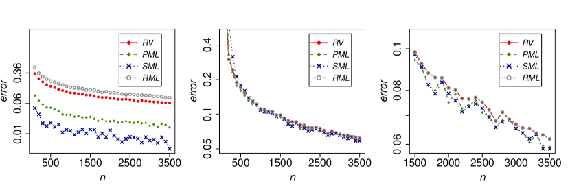
$\widehat{\mathbf{B}}$ coincides with ${\mathbf{B}}^{*}$ $\widehat{\mathbf{B}}$ estimated by SqRL$+$OLS $\widehat{\mathbf{B}}$ estimated by SqRL$+$OLS: zoom

Figure 1: The average $\ell_{2}$-error (computed from 50 independent trials) of the four estimators considered in this work as a function of the sample size. The plots concern Model 2 described in Section 4.1 and dimension $p=60$. One can observe, in particular, that when ${\mathbf{B}}^{*}$ is estimated without error (left panel), the estimators SML and PML improve on the residual variance and relaxed maximum likelihood estimators.

It follows from the above discussion that the problem of estimating the matrix ${\mathbf{D}}^{*}$ built from the diagonal entries of the precision matrix is an important ingredient of the estimation of the precision matrix and the graph of conditional dependencies between the features. The purpose of the present work is to propose several natural estimators of ${\mathbf{D}}^{*}$ and to study their statistical properties, essentially from an empirical point of view. Combining standard arguments, we present four estimators, termed residual variance (RV), relaxed maximum likelihood (RML), symmetry-enforced maximum likelihood (SML) and penalized maximum likelihood (PML). The first one, residual variance, is the most commonly used estimator when the matrix ${\mathbf{B}}^{*}$ is estimated column-wise by a sparse linear regression approach briefly mentioned in the foregoing discussion. The other three methods considered in this paper are based on the principle of likelihood maximization under various approaches for handling the prior information. In order to give the reader a foretaste of the content of next sections, we present in Figure 1 the accuracy of the four methods of estimating the diagonal elements of the precision matrix on a synthetic data-set. More details are given in Section 4.1.

2 Notation and preliminaries on precision matrix estimation

This section introduces notation used throughout the paper and presents some preliminary material on sparse precision matrix estimation.

2.1 Notation

For an unknown parameter $\theta$ we note $\theta^{*}$ its true value. As usual, $\mathcal{N}_{p}(\boldsymbol{\mu}^{*},\mathbf{\Sigma}^{*})$ is the Gaussian distribution in $\mathbb{R}^{p}$ with mean $\boldsymbol{\mu}^{*}$ and covariance matrix $\mathbf{\Sigma}^{*}$. The expectation of a random vector ${\mathbf{X}}$ is denoted by ${\mathbf{E}}({\mathbf{X}})$ and its covariance matrix by ${\mathbf{V}}({\mathbf{X}})$. We denote by ${\mathbf{1}}_{n}$ the vector from $\mathbb{R}^{n}$ with all the entries equal to $1$ and by ${\mathbf{I}}_{n}$ the $n\times n$ identity matrix. We write $\mathds{1}$ for the indicator function, which is equal to 1 if the considered condition is satisfied and 0 otherwise. The smallest integer greater than or equal to $x\in\mathbb{R}$ is denoted by $\lceil x\rceil$. In what follows, $[p]:=\{1,\ldots,p\}$ is the set of positive integers from $1$ to $p$. For $i\in[p]$, the complement of the singleton $\{i\}$ in $[p]$ is denoted by $i^{c}$. For a vector ${\boldsymbol{v}}\in\mathbb{R}^{p}$, ${\mathbf{D}}_{\boldsymbol{v}}$ stands for the $p\times p$ diagonal matrix satisfying $({\mathbf{D}}_{\boldsymbol{v}})_{j}={\boldsymbol{v}}_{j}$ for every $j\in[p]$. The matrix build keeping only the diagonal of a square matrix ${\mathbf{M}}$ is denoted by ${\rm diag}({\mathbf{M}})$.

The transpose of the matrix ${\mathbf{M}}$ is denoted by ${\mathbf{M}}^{\top}$. If this matrix is square, we note $|{\mathbf{M}}|$ its determinant. For a $n\times p$ matrix ${\mathbf{M}}$, the vector of the elements of the $k$th row (resp. the $j$th column) whose indices are given by the subset $J$ of $[p]$ (resp. $K$ of $[n]$) is denoted by ${\mathbf{M}}_{k,J}$ (resp. ${\mathbf{M}}_{K,j}$). In particular, the vector made of all the elements of the $j$th column of the matrix ${\mathbf{M}}$ at the exception of the element of the $k$th row is given by ${\mathbf{M}}_{k^{c},j}$. Moreover, the whole $k$th row (resp. $j$th column) of ${\mathbf{M}}$ is denoted by ${\mathbf{M}}_{k,\bullet}$ (resp. ${\mathbf{M}}_{\bullet,j}$). We use the following notation for the (pseudo-)norms of matrices: if $q_{1},q_{2}>0$, then

$${\|{\mathbf{M}}\|}_{q_{1},q_{2}}=\left\{\sum_{i=1}^{n}\|{\mathbf{M}}_{i,\bullet}\|_{q_{1}}^{q_{2}}\right\}^{1/q_{2}}.$$

With this notation, $\|{\mathbf{M}}\|_{2,2}$ and $\|{\mathbf{M}}\|_{1,1}$ are the Frobenius and the element-wise $\ell_{1}$-norm of ${\mathbf{M}}$, respectively. The sample covariance matrix of the data points $\{{\mathbf{X}}_{k,\bullet}\}_{k\in[n]}$ is defined by

$${\mathbf{S}}_{n}=\frac{1}{n}\sum_{k=1}^{n}({\mathbf{X}}_{k,\bullet}^{\top}-\widehat{\boldsymbol{\mu}})({\mathbf{X}}_{k,\bullet}^{\top}-\widehat{\boldsymbol{\mu}})^{\top}=\frac{1}{n}({\mathbf{X}}-{\mathbf{1}}_{n}\widehat{\boldsymbol{\mu}}^{\top})^{\top}({\mathbf{X}}-{\mathbf{1}}_{n}\widehat{\boldsymbol{\mu}}^{\top}),$$

where $\widehat{\boldsymbol{\mu}}$ is either the sample mean $\frac{1}{n}({\mathbf{1}}_{n}^{\top}{\mathbf{X}})^{\top}$ (when the mean $\boldsymbol{\mu}^{*}$ is unknown) or the theoretical mean $\boldsymbol{\mu}^{*}$ (when it is considered as known).

2.2 Preliminaries

Throughout the paper we will present estimators of the diagonal elements of the precision matrix in the case of a general multidimensional Gaussian distribution, but in all theoretical developments we will assume that the marginals of ${\mathbf{X}}$ are standard Gaussian distributions, i.e., $\boldsymbol{\mu}^{*}=0$ and $\mathbf{\Sigma}_{jj}^{*}=1$ for every $j\in[p]$. This assumption is reasonable, since we are concerned with the problems in which the sample size is large enough to consistently estimate the individual means and the individual variances of the variables. So, one can always center the variables by the sample mean and divide by the sample standard deviation to get close to the assumption that random variables ${\mathbf{X}}_{1,j},\ldots,{\mathbf{X}}_{n,j}$ are i.i.d. $\mathcal{N}(0,1)$ for every $j$.

Let us recall that the precision matrix is closely related to the problem of regression of one feature on all the others. Indeed, there exists a $p\times p$ matrix ${\mathbf{B}}^{*}$ and two vectors ${\mathbf{c}}^{*},\boldsymbol{\phi}^{*}\in\mathbb{R}^{p}$ such that

$${\mathbf{X}}_{\bullet,j}=c_{j}^{*}{\mathbf{1}}_{n}-{\mathbf{X}}_{\bullet,j^{c}}{\mathbf{B}}^{*}_{j^{c},j}+\phi_{j}^{*}{}^{1/2}\,\boldsymbol{\xi}_{j},$$ (1)

where $\boldsymbol{\xi}_{j}$ is drawn from $\mathcal{N}_{n}(0,{\mathbf{I}}_{n})$ and is independent of ${\mathbf{X}}_{\bullet,j^{c}}$. According to the theorem on normal correlations (Marsaglia, 1964), the regression coefficients ${\mathbf{B}}^{*}_{j^{c},j}\in\mathbb{R}^{p-1}$ and the variance $\phi^{*}_{j}\in\mathbb{R}$ of residuals can be expressed in terms of the elements of the precision matrix $\mathbf{\Omega}^{*}$ as follows:

$${\mathbf{B}}^{*}_{ij}={\omega^{*}_{ij}}/{\omega^{*}_{jj}},\qquad\phi^{*}_{j}=1/{\omega^{*}_{jj}},$$ (NC)

whereas $c_{j}^{*}=\mu_{j}^{*}+(\boldsymbol{\mu}_{j^{c}}^{*})^{\top}{\mathbf{B}}^{*}_{j^{c},j}=(\boldsymbol{\mu}^{*})^{\top}{\mathbf{B}}^{*}_{\bullet,j}$. If we assume that $\boldsymbol{\mu}^{*}=0$ then $c^{*}_{j}=0$ for any $j$. With these notation, the precision matrix can be written as $\mathbf{\Omega}^{*}={\mathbf{B}}^{*}{\mathbf{D}}_{\boldsymbol{\phi}^{*}}^{-1}$.

Several state-of-the-art methods for estimating sparse precision matrices proceed in two steps (Meinshausen and Bühlmann, 2006; Cai et al., 2011; Liu and Wang, 2012; Sun and Zhang, 2013). The first step consists in estimating the matrix ${\mathbf{B}}^{*}$ and the vector $\boldsymbol{\phi}^{*}$ by solving the sparse linear regression problems (1) for each $j$, while in the second step an estimator of the matrix $\mathbf{\Omega}^{*}$ is inferred from the estimators of ${\mathbf{B}}^{*}$ and $\boldsymbol{\phi}^{*}$ using relations (NC). The goal of the present work is to explore both theoretically and empirically different possible strategies for this second step.

The square-root Lasso is perhaps the method of estimating the matrix ${\mathbf{B}}^{*}$ that offers the best trade-off between the computational and the statistical complexities. It can be redefined as follows: scaled Lasso estimates the matrix ${\mathbf{B}}^{*}$ by solving the convex optimization problem

$$\widehat{\mathbf{B}}=\operatorname*{arg\,min}_{\begin{subarray}{c}{\mathbf{B}}\in\mathbb{R}^{p\times p}\\ {\mathbf{B}}_{jj}=1\end{subarray}}\limits\min_{{\mathbf{c}}\in\mathbb{R}^{p}}\Big{\{}{\|{\mathbf{X}}{\mathbf{B}}-{\mathbf{1}}_{n}{\mathbf{c}}^{\top}\|}_{2,1}+\lambda{\|{\mathbf{B}}\|}_{1,1}\Big{\}},$$ (2)

where the first $\min$ is over all matrices ${\mathbf{B}}$ having all their diagonal entries equal to $1$. The tuning parameter $\lambda>0$ corresponds to the penalty level. The purpose of the penalization is indeed to get a precision matrix estimate which fits the sparsity assumption. As the penalty of a matrix ${\mathbf{B}}$ is its $\|\cdot\|_{1,1}$ norm, the resulting precision matrix estimator is expected to be sparse in the sense that its overall number of non-zero elements should be small. In addition, one can check that computing a solution to problem (2) is equivalent to computing each column of $\widehat{\mathbf{B}}$ separately (and independently) by solving the optimization problem

$$\widehat{\mathbf{B}}_{\bullet,j}=\operatorname*{arg\,min}_{\begin{subarray}{c}\boldsymbol{\beta}\in\mathbb{R}^{p}\\ \boldsymbol{\beta}_{j}=1\end{subarray}}\limits\min_{c_{j}\in\mathbb{R}}\Big{\{}{\|{\mathbf{X}}\boldsymbol{\beta}_{j}-c_{j}{\mathbf{1}}_{n}\|}_{2}+\lambda{\|\boldsymbol{\beta}\|}_{1}\Big{\}},\quad j\in[p].$$ (3)

In addition to being efficiently computable even for large $p$, this estimator has the following appealing property that makes it preferable, for instance, to the column-wise Lasso (Meinshausen and Bühlmann, 2006) and the CLIME (Cai et al., 2011). The choice of the parameter $\lambda$ in (2-3) is scale free: it can be chosen independently of the noise variance in linear regression (1). This fact has been first established by Belloni et al. (2011) and then further investigated in (Sun and Zhang, 2012; Belloni et al., 2014a). In the context of precision matrix estimation, this method has been explored by Sun and Zhang (2013).

3 Four estimators of ${\mathbf{\phi}^{*}}$

As mentioned earlier, the aim of this work is to compare different estimators of the vector $\boldsymbol{\phi}^{*}$ based on an initial estimator of the matrix ${\mathbf{B}}^{*}$. Clearly, the error of the estimation of ${\mathbf{B}}^{*}$ impacts the error of the estimation of $\boldsymbol{\phi}^{*}$ and, therefore, the latter is not easy to assess in full generality. In order to gain some insight on the behavior of various natural estimators, in theoretical results we will consider the ideal situation where the matrix ${\mathbf{B}}^{*}$ is estimated without error.

3.1 Residual variance estimator

In view of the regression equation (1), a standard and natural method—used, in particular, by the square-root Lasso of Sun and Zhang (2013)—to deduce estimators $\widehat{\boldsymbol{\phi}}$ and $\widehat{\mathbf{\Omega}}$ from an estimator $\widehat{\mathbf{B}}$ is to set

$$\widehat{\phi}_{j}=\frac{1}{n}{\|({\mathbf{I}}_{n}-n^{-1}{\mathbf{1}}_{n}{\mathbf{1}}^{\top}_{n}){\mathbf{X}}\widehat{\mathbf{B}}_{\bullet,j}\|}_{2}^{2};\qquad\widehat{\mathbf{\Omega}}=\widehat{\mathbf{B}}\cdot{\mathbf{D}}_{\widehat{\boldsymbol{\phi}}}^{-1}.$$ (4)

Note that the matrix $({\mathbf{I}}_{n}-n^{-1}{\mathbf{1}}_{n}{\mathbf{1}}^{\top}_{n})$ present in this expression is the orthogonal projector in $\mathbb{R}^{n}$ onto the orthogonal complement of the linear subspace $\text{Span}({\mathbf{1}}_{n})$ of all constant vectors. The multiplication by this matrix annihilates the intercept $c_{j}^{*}$ in (1) and is a standard way of reducing the affine regression to the linear regression. In what follows, we refer to $\widehat{\boldsymbol{\phi}}$ defined by (4) as the residual variance estimator and denote it by $\widehat{\boldsymbol{\phi}}{}^{{\,\rm RV}}$. Using the sample covariance matrix ${\mathbf{S}}_{n}$, the residual variance estimator of $\boldsymbol{\phi}^{*}$ can be written as

$$\widehat{\phi}^{{\,\rm RV}}_{j}=\widehat{\mathbf{B}}_{\bullet,j}^{\top}{\mathbf{S}}_{n}\widehat{\mathbf{B}}_{\bullet,j}.$$

Note also that if we consider the linear regression model (1) conditionally to ${\mathbf{X}}_{\bullet,j^{c}}$, then the residual variance estimator of $\phi_{j}^{*}$ coincides with the maximum likelihood estimator.

Proposition 1.

If $\widehat{\mathbf{B}}_{\bullet,j}$ estimates ${\mathbf{B}}^{*}_{\bullet,j}$ without error, then the residual variance estimator of $\phi^{*}_{j}$ has a quadratic risk equal to $\frac{2}{n}{\phi_{j}^{*}}^{2}$, that is

$${\mathbf{E}}[(\widehat{\phi}^{{\,\rm RV}}_{j}-\phi^{*}_{j})^{2}]=\frac{2\phi_{j}^{*}{}^{2}}{n}.$$

Furthermore, for every $t>0$, the following bound on the tails of the maximal error holds true:

$${\mathbf{P}}\bigg{(}\max_{j\in[p]}\frac{|\widehat{\phi}^{{\,\rm RV}}_{j}-\phi^{*}_{j}|}{\phi^{*}_{j}}>2\Big{(}\frac{t+\log p}{n}\Big{)}^{1/2}+\frac{2(t+\log p)}{n}\bigg{)}\leq 2e^{-t}.$$

Proof.

Using equation (1) and the assumption $\widehat{\mathbf{B}}_{\bullet,j}={\mathbf{B}}^{*}_{\bullet,j}$, we get

$$\widehat{\phi}^{{\,\rm RV}}_{j}=\frac{1}{n}{\|{\mathbf{X}}{\mathbf{B}}^{*}_{\bullet,j}\|}_{2}^{2}=\frac{\phi_{j}^{*}}{n}{\|\boldsymbol{\xi}_{j}\|}_{2}^{2}.$$ (5)

Since $\boldsymbol{\xi}_{j}$ is a standard Gaussian vector, the random variable $\zeta={\|\boldsymbol{\xi}_{j}\|}_{2}^{2}$ is drawn from a $\chi^{2}_{n}$ distribution. This implies that ${\mathbf{E}}(\zeta)=n$ and ${\mathbf{V}}(\zeta)=2n$. Therefore,

$${\mathbf{E}}[(\widehat{\phi}^{{\,\rm RV}}_{j}-\phi^{*}_{j})^{2}]={\mathbf{E}}\Big{[}\Big{(}\frac{\phi_{j}^{*}\zeta}{n}-\phi^{*}_{j}\Big{)}^{2}\Big{]}=\frac{\phi^{*}_{j}{}^{2}}{n^{2}}\Big{(}{\mathbf{V}}(\zeta)+\big{(}{\mathbf{E}}(\zeta)-n\big{)}^{2}\Big{)}=\frac{2\phi^{*}_{j}{}^{2}}{n}.$$

This completes the proof of the first claim. To prove the second claim, we set $z=t+\log p$ and use the union bound to get

$${\mathbf{P}}\bigg{(}\max_{j\in[p]}\frac{|\widehat{\phi}^{{\,\rm RV}}_{j}-\phi^{*}_{j}|}{\phi^{*}_{j}}>2\sqrt{\frac{z}{n}}+\frac{2z}{n}\bigg{)} \leq p\max_{j\in[p]}{\mathbf{P}}\bigg{(}\frac{|\widehat{\phi}^{{\,\rm RV}}_{j}-\phi^{*}_{j}|}{\phi^{*}_{j}}>2\sqrt{\frac{z}{n}}+\frac{2z}{n}\bigg{)}$$

$$=p{\mathbf{P}}\big{(}|\zeta-n|>2\sqrt{zn}+2z\big{)}.$$

The second claim follows from the tail bound of the $\chi^{2}$ distribution established, for instance, in (Laurent and Massart, 2000, Lemma 1). ∎

Note that in this result, the case of known means $\mu_{j}^{*}$ is considered. The case of unknown $\mu_{j}$ can be handled similarly, the estimation bias is then $\phi_{j}^{*}/n$ and the resulting mean squared error is $(2n-1)\phi_{j}^{*}{}^{2}/n^{2}$. One may observe that, as expected, the rate of convergence of the quadratic risk is the usual parametric rate $1/n$ and that the asymptotic variance is $2\phi_{j}^{*}{}^{2}$.

3.2 Relaxed maximum likelihood estimator

One could expect that the global maximum likelihood estimator of $\boldsymbol{\phi}^{*}$ would be better than the maximum of the conditional likelihood, since it is well known that under proper regularity conditions, the quadratic risk of the maximum likelihood estimator is the smallest, at least asymptotically. Since the vectors ${\mathbf{X}}_{k,\bullet}\sim\mathcal{N}_{p}(\boldsymbol{\mu}^{*},\mathbf{\Omega}^{*}{}^{-1})$ are independent, the log-likelihood is given by (up to irrelevant additive terms independent of the unknown parameters $\boldsymbol{\mu}^{*}$ and $\mathbf{\Omega}^{*}$)

$$\mathcal{L}({\mathbf{X}}|\boldsymbol{\mu},\mathbf{\Omega})=\frac{n}{2}\log|\mathbf{\Omega}|-\frac{1}{2}\sum_{k=1}^{n}({\mathbf{X}}_{k,\bullet}-\boldsymbol{\mu}^{\top})\mathbf{\Omega}({\mathbf{X}}_{k,\bullet}-\boldsymbol{\mu}^{\top})^{\top}.$$ (6)

Maximizing the log-likelihood with respect to $\boldsymbol{\mu}\in\mathbb{R}^{p}$ leads to

$$\max_{\boldsymbol{\mu}\in\mathbb{R}^{p}}\mathcal{L}({\mathbf{X}}|\boldsymbol{\mu},\mathbf{\Omega})=\frac{n}{2}\Big{(}\log|\mathbf{\Omega}|-\text{\rm trace}\big{[}{\mathbf{S}}_{n}\mathbf{\Omega}\big{]}\Big{)}.$$ (7)

Recall now that in view of (NC), we have $\mathbf{\Omega}^{*}={\mathbf{B}}^{*}{\mathbf{D}}_{\boldsymbol{\phi}^{*}}^{-1}$. Therefore, the profiled log-likelihood (w.r.t. $\boldsymbol{\mu}$) of ${\mathbf{X}}$ given the parameters ${\mathbf{B}}$ and $\boldsymbol{\phi}$ is

$$\max_{\boldsymbol{\mu}\in\mathbb{R}^{p}}\mathcal{L}({\mathbf{X}}|\boldsymbol{\mu},{\mathbf{B}},\boldsymbol{\phi})=\frac{n}{2}\Big{(}\log|{\mathbf{B}}|-\sum_{j=1}^{p}\big{\{}\log(\phi_{j})+{({\mathbf{S}}_{n}{\mathbf{B}})}_{jj}\phi_{j}^{-1}\big{\}}\Big{)}.$$ (8)

For a given ${\mathbf{B}}$, this profiled log-likelihood is a decomposable function of $\boldsymbol{\phi}$ and, therefore, can be easily maximized with respect to $\boldsymbol{\phi}$. This leads to

$$\text{arg}\max_{\boldsymbol{\phi}\in\mathbb{R}_{+}^{p}}\max_{\boldsymbol{\mu}\in\mathbb{R}^{p}}\mathcal{L}({\mathbf{X}}|\boldsymbol{\mu},{\mathbf{B}},\boldsymbol{\phi})=\big{(}({\mathbf{S}}_{n}{\mathbf{B}})_{jj}\vee 0\big{)}_{j\in[p]}.$$ (9)

Thus, when an estimator $\widehat{\mathbf{B}}$ of ${\mathbf{B}}^{*}$ is available, one possible approach for estimating $\boldsymbol{\phi}^{*}$ is to set

$$\widehat{\phi}^{\,\rm RML}_{j}=({\mathbf{S}}_{n}\widehat{\mathbf{B}})_{jj}\vee 0,\qquad j\in[p].$$ (10)

We call this estimator relaxed maximum likelihood (RML) estimator. It will be clear a little bit later why it is called relaxed. The analysis of the risk of the RML estimator is more involved than that of the RV estimator considered in the previous section. This is due to the truncation at the level $0$. For this reason, the next result does not provide the precise value of the risk, but just an inequality which is sufficient for our purposes.

Proposition 2.

If $\widehat{\mathbf{B}}$ estimates ${\mathbf{B}}^{*}_{\bullet,j}$ without error, then the risk of the RML estimator of $\phi_{j}^{*}$ satisfies ${\mathbf{E}}[(\widehat{\phi}^{\,\rm RML}_{j}-\phi^{*}_{j})^{2}]\geq\frac{1}{n}\big{(}{\phi_{j}^{*}}^{2}+\phi_{j}^{*}\mathbf{\Sigma}^{*}_{jj}-O(n^{-1/2})\big{)}$.

Before providing the proof of this result, let us present a brief discussion. Note that in view of (1), $\mathbf{\Sigma}^{*}_{jj}$ is always not smaller than $\phi_{j}^{*}$. Furthermore, $\mathbf{\Sigma}^{*}_{jj}>\phi_{j}^{*}$ if ${\mathbf{B}}^{*}_{j^{c},j}$ has at least one nonzero entry. Therefore, the last proposition, combined with Proposition 1, establishes that the residual variance estimator has an asymptotic variance which is smaller (and, in many cases, strictly smaller) than the asymptotic variance of the maximum likelihood estimator. At a first sight, this is very surprising and seems to be in contradiction with the well established theory (Le Cam and Yang, 2000; Ibragimov and Has^′minskiĭ, 1981) of asymptotic efficiency of the maximum likelihood estimator for regular models. Our explanation of this inefficiency of $\widehat{\phi}^{\,\rm RML}_{j}$ is that it is not really the maximum likelihood estimator. It maximizes the likelihood, certainly, but not over the correct set of parameters. Indeed, when we defined the RML we neglected an important property of the vector $\boldsymbol{\phi}^{*}$: the fact that ${\mathbf{B}}^{*}{\mathbf{D}}_{\boldsymbol{\phi}^{*}}^{-1}={\mathbf{D}}_{\boldsymbol{\phi}^{*}}^{-1}{\mathbf{B}}^{*}{}^{\top}$ (this follows from the symmetry of $\mathbf{\Omega}^{*}$). Ignoring this constraint allowed us to get a tractable optimization problem but caused the loss of the (asymptotic) efficiency of the estimator. This also explains why we call $\widehat{\boldsymbol{\phi}}{}^{\,\rm RML}$ relaxed maximum likelihood estimator.

Proof of Proposition 2.

Since $\boldsymbol{\mu}^{*}$ is assumed to be known and equal to zero, according to (1), we have

$$({\mathbf{S}}_{n}\widehat{\mathbf{B}})_{jj}=\frac{1}{n}{\mathbf{X}}_{\bullet,j}^{\top}{\mathbf{X}}{\mathbf{B}}^{*}_{\bullet,j}=\frac{\phi_{j}^{*}{}^{1/2}}{n}{\mathbf{X}}_{\bullet,j}^{\top}\boldsymbol{\xi}_{j}=\frac{\phi_{j}^{*}{}^{1/2}}{n}\big{(}-{\mathbf{X}}_{\bullet,j^{c}}{\mathbf{B}}^{*}_{j^{c},j}+\phi_{j}^{*}{}^{1/2}\;\boldsymbol{\xi}_{j}\big{)}^{\top}\boldsymbol{\xi}_{j}.$$

Denoting $\eta_{1}=-\boldsymbol{\xi}_{j}^{\top}{\mathbf{X}}_{\bullet,j^{c}}{\mathbf{B}}^{*}_{j^{c},j}$, we get $({\mathbf{S}}_{n}\widehat{\mathbf{B}})_{jj}=\frac{1}{n}({\phi_{j}^{*}{}^{1/2}}\;\eta_{1}+{{\phi_{j}^{*}}}\;\|\boldsymbol{\xi}_{j}\|_{2}^{2})$. Furthermore, it follows from (1) that ${\mathbf{E}}[({\mathbf{X}}_{k,j^{c}}{\mathbf{B}}^{*}_{j^{c},j})^{2}]=\mathbf{\Sigma}_{jj}^{*}-\phi_{j}^{*}$ for each $k$. Since, in addition, for different $k$s the random variables ${\mathbf{X}}_{k,j^{c}}{\mathbf{B}}^{*}_{j^{c},j}$ are independent, centered and Gaussian, we get that—in view of the independence of $\boldsymbol{\xi}_{j}$ and ${\mathbf{X}}_{\bullet,j^{c}}$—the conditional distribution of $\eta_{1}$ given $\boldsymbol{\xi}_{j}$ is Gaussian with zero mean and variance $\|\boldsymbol{\xi}_{j}\|_{2}^{2}(\mathbf{\Sigma}^{*}_{jj}-\phi_{j}^{*})$. Hence, the random variable $\eta=\eta_{1}/(\|\boldsymbol{\xi}_{j}\|_{2}(\mathbf{\Sigma}^{*}_{jj}-\phi_{j}^{*})^{1/2})$ is standard Gaussian, independent of $\|\boldsymbol{\xi}_{j}\|_{2}^{2}$ and

$$({\mathbf{S}}_{n}\widehat{\mathbf{B}})_{jj}=\frac{\sqrt{\phi_{j}^{*}\|\boldsymbol{\xi}_{j}\|_{2}^{2}(\mathbf{\Sigma}^{*}_{jj}-\phi_{j}^{*})}}{n}\;\eta+\frac{{\phi_{j}^{*}}}{n}\;\|\boldsymbol{\xi}_{j}\|_{2}^{2}.$$

This relation readily implies that ${\mathbf{E}}[({\mathbf{S}}_{n}\widehat{\mathbf{B}})_{jj}]=\phi_{j}^{*}$ and

$${\mathbf{E}}[(({\mathbf{S}}_{n}\widehat{\mathbf{B}})_{jj}-\phi_{j}^{*})^{2}]={\mathbf{V}}[({\mathbf{S}}_{n}\widehat{\mathbf{B}})_{jj}]=\frac{\mathbf{\Sigma}_{jj}^{*}\phi_{j}^{*}+\phi_{j}^{*}{}^{2}}{n}.$$

Furthermore, for the fourth moment, we have

$${\mathbf{E}}[(({\mathbf{S}}_{n}\widehat{\mathbf{B}})_{jj}-\phi_{j}^{*})^{4}] \leq\frac{8\phi_{j}^{*}{}^{2}(\mathbf{\Sigma}^{*}_{jj}-\phi_{j}^{*})^{2}}{n^{4}}{\mathbf{E}}[\|\boldsymbol{\xi}_{j}\|_{2}^{4}]{\mathbf{E}}[\eta^{4}]+\frac{8\phi_{j}^{*}{}^{4}}{n^{4}}\;{\mathbf{E}}[(\|\boldsymbol{\xi}_{j}\|_{2}^{2}-n)^{4}]$$

$$\leq\frac{72\phi_{j}^{*}{}^{2}(\mathbf{\Sigma}^{*}_{jj}-\phi_{j}^{*})^{2}}{n^{2}}+\frac{8\phi_{j}^{*}{}^{4}}{n^{4}}(60n+12n^{2}).$$

To analyze the truncated estimator, we set $\zeta=({\mathbf{S}}_{n}\widehat{\mathbf{B}})_{jj}$. Then $\widehat{\phi}^{\,\rm RML}_{j}=\zeta\cdot\mathds{1}(\zeta>0)$ and hence,

$${\mathbf{E}}[(\widehat{\phi}^{\,\rm RML}_{j}-\phi_{j}^{*})^{2}] ={\mathbf{E}}[(\zeta-\phi_{j}^{*})^{2}\mathds{1}(\zeta>0)]+\phi_{j}^{*}{}^{2}{\mathbf{P}}(\zeta\leq 0)$$

$$={\mathbf{E}}[(\zeta-\phi_{j}^{*})^{2}]-{\mathbf{E}}[(\zeta-\phi_{j}^{*})^{2}\mathds{1}(\zeta\leq 0)]+\phi_{j}^{*}{}^{2}{\mathbf{P}}(\zeta\leq 0)$$

$$\geq{\mathbf{E}}[(\zeta-\phi_{j}^{*})^{2}]-{\mathbf{E}}[(\zeta-\phi_{j}^{*})^{4}]^{1/2}{\mathbf{P}}(\zeta\leq 0)^{1/2}.$$

We have already computed the first expectation in the right-hand side, as well as upper bounded the second one. Let us show that the probability of the event $\zeta\leq 0$ goes to zero as $n$ increases to $\infty$. This follows from the Tchebychev inequality, since ${\mathbf{P}}(\zeta\leq 0)={\mathbf{P}}(\phi_{j}^{*}-\zeta\geq\phi_{j}^{*})\leq{\mathbf{V}}[\zeta]/\phi_{j}^{*}{}^{2}=O(1/n)$. This completes the proof of the proposition. ∎

3.3 MLE taking into account the symmetry constraints

As we have seen in previous sections, the relaxed maximum likelihood estimator is suboptimal; in particular, it is less accurate than the residual variance estimator. To check that this lack of efficiency is indeed due to the relaxation of the symmetry constraints, we propose here to analyze the constrained maximum likelihood estimator in the following idealized set-up. We will consider, as in Propositions 1 and 2, that $\widehat{\mathbf{B}}$ estimates ${\mathbf{B}}^{*}$ without error, and that there is a column ${\mathbf{B}}^{*}_{\bullet,i}$ in ${\mathbf{B}}^{*}$ such that all the elements of ${\mathbf{B}}^{*}_{\bullet,i}$ are different from zero. Without loss of generality, we suppose that $i=1$ and, consequently, for every $j\in[p]$, we have ${\mathbf{B}}^{*}_{j1}\neq 0$ which is equivalent to $\omega^{*}_{j1}\neq 0$. Therefore, the symmetry constraint ${\mathbf{B}}^{*}{\mathbf{D}}_{\boldsymbol{\phi}^{*}}^{-1}=\mathbf{\Omega}^{*}=\mathbf{\Omega}^{*}{}^{\top}={\mathbf{D}}_{\boldsymbol{\phi}^{*}}^{-1}{\mathbf{B}}^{*}{}^{\top}$ implies that ${\mathbf{D}}_{\boldsymbol{\phi}^{*}}{\mathbf{B}}^{*}={\mathbf{B}}^{*}{}^{\top}{\mathbf{D}}_{\boldsymbol{\phi}^{*}}$ and, in particular, that

$${\mathbf{B}}^{*}_{1j}\phi_{1}^{*}={\mathbf{B}}^{*}_{j1}\phi_{j}^{*},\qquad\forall j\in[p].$$

This relation entails that in the case of known matrix ${\mathbf{B}}^{*}$ and unknown vector $\boldsymbol{\phi}^{*}$, only the first entry of $\boldsymbol{\phi}^{*}$ needs to be estimated, all the remaining entries can be computed using the first one by the formula $\widehat{\phi}_{j}=({\mathbf{B}}^{*}_{1j}/{\mathbf{B}}^{*}_{j1})\widehat{\phi}_{1}$.

Proposition 3.

Under the assumption that the rows of ${\mathbf{X}}$ are i.i.d. Gaussian vectors with precision matrix $\mathbf{\Omega}^{*}={\mathbf{B}}^{*}{\mathbf{D}}_{\boldsymbol{\phi}^{*}}^{-1}$, the maximum likelihood estimator of $\boldsymbol{\phi}^{*}$ is defined by

$$\widehat{\phi}^{\,\rm SML}_{j}=\frac{1}{p}({\mathbf{B}}^{*}_{1j}/{\mathbf{B}}^{*}_{j1})\text{\rm trace}\big{(}{\mathbf{S}}_{n}{\mathbf{B}}^{*}{\mathbf{D}}_{{\mathbf{B}}^{*}_{\bullet,1}}{\mathbf{D}}_{{\mathbf{B}}^{*}_{1,\bullet}}^{-1}\big{)}.$$ (11)

The quadratic risk of this estimator is given by

$${\mathbf{E}}[(\widehat{\phi}^{\,\rm SML}_{j}-\phi_{j}^{*})^{2}]=\frac{2}{np}\;\phi_{j}^{*}{}^{2}.$$ (12)

Furthermore, for every $t>0$, the following bound on the tails of the maximal error holds true:

$${\mathbf{P}}\bigg{(}\max_{j\in[p]}\frac{|\widehat{\phi}^{\,\rm SML}_{j}-\phi^{*}_{j}|}{\phi^{*}_{j}}>2\Big{(}\frac{t+\log p}{np}\Big{)}^{1/2}+\frac{2(t+\log p)}{np}\bigg{)}\leq 2e^{-t}.$$

Proof.

To ease notation, we denote by ${\mathbf{D}}^{*}$ the diagonal matrix whose $j$th element is ${\mathbf{B}}^{*}_{j,1}/{\mathbf{B}}^{*}_{1,j}$. Then, applying (8) for a given ${\mathbf{B}}^{*}$, the profiled Gaussian log-likelihood can be written as

$$\max_{\boldsymbol{\mu}\in\mathbb{R}^{p}}\mathcal{L}({\mathbf{X}}|\boldsymbol{\mu},{\mathbf{B}}^{*},\boldsymbol{\phi})=\frac{n}{2}\log|{\mathbf{B}}^{*}|-\frac{n}{2}\sum_{j=1}^{p}\big{\{}\log(\phi_{j})+({\mathbf{S}}_{n}{\mathbf{B}}^{*})_{jj}\phi_{j}^{-1}\big{\}}.$$

The goal is to maximize the right-hand side over all the vectors $\boldsymbol{\phi}\in\mathbb{R}^{p}$ such that ${\mathbf{B}}^{*}{\mathbf{D}}_{\boldsymbol{\phi}}^{-1}$ is a valid precision matrix.

Let us first check that under the conditions of the proposition, for ${\mathbf{B}}^{*}{\mathbf{D}}_{\boldsymbol{\phi}}^{-1}$ to be a valid precision matrix it is necessary and sufficient that $\phi_{1}>0$ and $\phi_{j}=({\mathbf{B}}^{*}_{1j}/{\mathbf{B}}^{*}_{j1})\phi_{1}$ for every $j\in[p]$. The necessary part follows from that fact that a precision matrix is symmetric and positive-semidefinite, which entails that $({\mathbf{B}}^{*}{\mathbf{D}}_{\boldsymbol{\phi}}^{-1})_{1j}=({\mathbf{B}}^{*}{\mathbf{D}}_{\boldsymbol{\phi}}^{-1})_{j1}$ and $({\mathbf{B}}^{*}{\mathbf{D}}_{\boldsymbol{\phi}}^{-1})_{jj}=\boldsymbol{\phi}_{j}^{-1}>0$. Therefore, $\phi_{j}=({\mathbf{B}}^{*}_{1j}/{\mathbf{B}}^{*}_{j1})\phi_{1}$ and $\phi_{1}>0$. To check the sufficient part, we remark that if $\boldsymbol{\phi}$ satisfies $\phi_{j}=({\mathbf{B}}^{*}_{1j}/{\mathbf{B}}^{*}_{j1})\phi_{1}$ with $\phi_{1}>0$, then ${\mathbf{B}}^{*}{\mathbf{D}}_{\boldsymbol{\phi}}^{-1}=(\phi^{*}_{1}/\phi_{1}){\mathbf{B}}^{*}{\mathbf{D}}_{\boldsymbol{\phi}^{*}}^{-1}=(\phi^{*}_{1}/\phi_{1})\mathbf{\Omega}^{*}$. This implies that ${\mathbf{B}}^{*}{\mathbf{D}}_{\boldsymbol{\phi}}^{-1}$ is symmetric and positive-semidefinite, hence a valid precision matrix.

The maximum likelihood estimator $\widehat{\boldsymbol{\phi}}{}^{\,\rm SML}$ is thus given by

$$\widehat{\boldsymbol{\phi}}{}^{\,\rm SML}\in\text{arg}\min_{\begin{subarray}{c}\boldsymbol{\phi}\in\mathbb{R}^{p}_{+}\\ \phi_{j}=({\mathbf{B}}^{*}_{1j}/{\mathbf{B}}^{*}_{j1})\phi_{1}\end{subarray}}\sum_{j=1}^{p}\big{\{}\log(\phi_{j})+({\mathbf{S}}_{n}{\mathbf{B}}^{*})_{jj}\phi_{j}^{-1}\big{\}},$$

which leads to $\widehat{\phi}^{\,\rm SML}_{1}\in\text{arg}\min_{\phi_{1}>0}\big{\{}p\log(\phi_{1})+\phi_{1}^{-1}\sum_{j}({\mathbf{S}}_{n}{\mathbf{B}}^{*})_{jj}{\mathbf{B}}_{j1}^{*}/{\mathbf{B}}^{*}_{1j}\big{\}}$. The cost function of the last minimization problem is convex, since we have $({\mathbf{S}}_{n}{\mathbf{B}}^{*})_{jj}{\mathbf{B}}_{j1}^{*}/{\mathbf{B}}^{*}_{1j}=({\mathbf{S}}_{n}{\mathbf{B}}^{*})_{jj}\phi_{1}^{*}/\phi^{*}_{j}=\phi_{1}^{*}({\mathbf{S}}_{n}\mathbf{\Omega}^{*})_{jj}$. This implies that

$$\sum_{j}({\mathbf{S}}_{n}{\mathbf{B}}^{*})_{jj}{\mathbf{B}}_{j1}^{*}/{\mathbf{B}}^{*}_{1j}=\phi_{1}^{*}\text{\rm trace}({\mathbf{S}}_{n}\mathbf{\Omega}^{*})=\phi_{1}^{*}\text{\rm trace}(\mathbf{\Omega}^{*}{}^{1/2}{\mathbf{S}}_{n}\mathbf{\Omega}^{*}{}^{1/2})\geq 0.$$

The aforementioned cost function is continuously differentiable and convex, its minimum is attained at the point where the derivative vanishes, which provides $\widehat{\phi}^{\,\rm SML}_{1}=\frac{1}{p}\sum_{j}({\mathbf{S}}_{n}{\mathbf{B}}^{*})_{jj}{\mathbf{B}}_{j1}^{*}/{\mathbf{B}}^{*}_{1j}$. Combining with the relation $\widehat{\phi}^{\,\rm SML}_{j}=({\mathbf{B}}^{*}_{1j}/{\mathbf{B}}^{*}_{j1})\widehat{\phi}^{\,\rm SML}_{1}$, this leads to (11).

To check (12), we start by noting that

$$\widehat{\phi}^{\,\rm SML}_{j}=\frac{1}{p}\phi^{*}_{j}\text{\rm trace}({\mathbf{S}}_{n}\mathbf{\Omega}^{*})=\frac{1}{np}\phi^{*}_{j}\text{\rm trace}({\mathbf{X}}^{\top}{\mathbf{X}}\mathbf{\Sigma}^{*}{}^{-1}).$$

Using the well-known commutativity property of the trace operator and setting ${\mathbf{Y}}=\mathbf{\Sigma}^{*}{}^{-1/2}{\mathbf{X}}^{\top}$, we get $\text{\rm trace}({\mathbf{X}}^{\top}{\mathbf{X}}\mathbf{\Sigma}^{*}{}^{-1})=\text{\rm trace}({\mathbf{Y}}^{\top}{\mathbf{Y}})$. Since ${\mathbf{X}}$ has iid rows drawn from a $\mathcal{N}_{p}(0,\mathbf{\Sigma}^{*})$ distribution, ${\mathbf{Y}}$ has iid columns drawn from $\mathcal{N}_{p}(0,{\mathbf{I}}_{p})$ distribution. Hence, the random variable $\text{\rm trace}({\mathbf{Y}}^{\top}{\mathbf{Y}})=\sum_{j\in[p],k\in[n]}{\mathbf{Y}}_{jk}^{2}$ is distributed according to $\chi^{2}_{np}$ distribution. This readily implies that $\widehat{\phi}^{\,\rm SML}_{j}$ is an unbiased estimator of $\phi_{j}^{*}$ and, therefore, its quadratic risk coincides with its variance and is given by (12).

The proof of the last claim of the proposition is very similar to that of the second claim of Proposition 1. ∎

Assuming that there exists $i\in[p]$ such that for any $j\in[p]$, $\omega^{*}_{ij}\neq 0$, put differently that the $i$-th node of the graph $\mathscr{G}^{*}$ is connected by an edge to any other node is quite restrictive. Among other implications, it entails that the graph $\mathscr{G}^{*}$ is connected which might be a strong assumption. It is therefore useful to adapt what precedes to the case where the graph $\mathscr{G}^{*}$ has more than one connected component. The rest of this subsection is devoted to the description of this adaptation.

We note $\mathscr{C}$ the set of the connected components of the graph $\mathscr{G}^{*}$. Each connected component $c\in\mathscr{C}$ is a subset of vertices of $\mathscr{G}^{*}$ whose cardinality is denoted by $p_{c}$. Clearly, the sum of $p_{c}$ over all $c\in\mathscr{C}$ equals $p$. For two vertices $i$ and $j$, we will write $i\sim_{\mathscr{G}^{*}\!}j$ for indicating that they belong to the same connected component. Thus, each connected component is a class of equivalence with respect to the relation $\sim_{\mathscr{G}^{*}\!}$. Let $i\sim_{\mathscr{G}^{*}\!}j$ be two vertices from $c\in\mathscr{C}$ and let $C_{ji}$ be a path connecting these two vertices,i.e., $C_{ji}$ is a sequence of $q$ distinct vertices $\{v_{1},\ldots,v_{q}\}$ such that $v_{1}=j$, $v_{q}=i$, $q\leq p_{c}$ and each pair $(v_{h},v_{h+1})$ is connected by an edge in $\mathscr{G}^{*}$. Recall that the symmetry of the precision matrix $\mathbf{\Omega}^{*}={\mathbf{B}}^{*}{\mathbf{D}}^{-1}_{\boldsymbol{\phi}^{*}}$ implies that ${\mathbf{B}}^{*}_{v_{h},v_{h+1}}\phi^{*}_{v_{h}}={\mathbf{B}}^{*}_{v_{h+1},v_{h}}\phi^{*}_{v_{h+1}}$ for every $h\in[q-1]$. This readily yields

$$\phi^{*}_{j}=\phi^{*}_{i}\prod_{1\leq h<q}\big{(}{\mathbf{B}}^{*}_{v_{h+1},v_{h}}/{\mathbf{B}}^{*}_{v_{h},v_{h+1}}\big{)}.$$

To ease notation, we introduce the $p\times p$ diagonal matrix $\mathbf{\Delta}_{j}^{*}$ the diagonal entries of which are defined by

$$(\mathbf{\Delta}_{j}^{*})_{ii}=\mathds{1}(i\sim_{\mathscr{G}^{*}}\!j)\prod_{1\leq h<q}\big{(}{\mathbf{B}}^{*}_{v_{h+1},v_{h}}/{\mathbf{B}}^{*}_{v_{h},v_{h+1}}\big{)},$$ (13)

where $\{v_{1},\ldots,v_{q}\}=C_{ji}$ is any path connecting $j$ to $i$ in $\mathscr{G}^{*}$. With this notation, $\phi^{*}_{j}=(\mathbf{\Delta}_{j}^{*})_{ii}\phi^{*}_{i}$. One can reproduce the arguments of the proof of Proposition 3 to check that the maximum likelihood estimator of $\boldsymbol{\phi}^{*}$, if ${\mathbf{B}}^{*}$ is known (and therefore so is $\mathbf{\Delta}_{j}^{*}$), is defined by

$$\widehat{\phi}^{\,\rm SML}_{j}=\frac{1}{p_{c}}\text{\rm trace}\big{(}\mathbf{\Delta}_{j}^{*}{\mathbf{S}}_{n}{\mathbf{B}}^{*}\big{)},$$ (14)

for $j$ belonging to the connected component $c$.

Comparing the results of Propositions 1, 2 and 3, we observe that the RV-estimator outperforms the RML estimator, but—at least in the case where there is a column in ${\mathbf{B}}^{*}$ which has only nonzero entries—they are both dominated by the maximum likelihood estimator that takes advantage of the symmetry constraints. Furthermore, using the same type of arguments as those of Proposition 3, one can check that if the vertex $j$ of the graph $\mathscr{G}^{*}$ belongs to a connected component of cardinal $p_{c}$ then the risk of the MLE in the ideal case of known ${\mathbf{B}}^{*}$ is equal to $\frac{2}{np_{c}}\phi_{j}^{*}{}^{2}$. This shows that in the ideal case the MLE systematically outperforms the widely used residual variance estimator, and the gain in the risk may be huge for vertices belonging to large connected components. On the other extreme, all the three estimators discussed in the previous section coincide when the matrix ${\mathbf{B}}^{*}$ is diagonal.

In order to apply equation (14) for estimating $\boldsymbol{\phi}^{*}$ when an estimator $\widehat{\mathbf{B}}$ of ${\mathbf{B}}^{*}$ is available, we need to construct an estimator $\widehat{\mathscr{G}}$ of the graph $\mathscr{G}^{*}$. We propose here an original approach for deriving $\widehat{\mathscr{G}}$ from $\widehat{\mathbf{B}}$. It is based on the observation that ${\mathbf{B}}^{*}_{ij}{\mathbf{B}}^{*}_{ji}={\omega^{*}_{ij}}^{2}/(\omega_{ii}^{*}\omega_{jj}^{*})^{2}$, the square of the partial correlation between the $i$-th and $j$-th variables. As mentioned earlier, this quantity is always between 0 and 1 and provides a convenient rule of selection for the edges to keep in the graph. More precisely, we connect $i$ to $j$ if the estimated squared partial correlation $\widehat{\mathbf{B}}_{ij}\widehat{\mathbf{B}}_{ji}$ is larger than a prescribed threshold $t\in(0,1)$. In our implementation, we chose (somewhat arbitrarily) the threshold $t=0.01\wedge n^{-1/2}$.

Note that when ${\mathbf{B}}^{*}$ is replaced by an estimator, the right-hand side of (14) is not necessarily invariant with respect to the choice of the path connecting $i$ to $j$. Therefore, even when $\widehat{\mathbf{B}}$ and $\widehat{\mathscr{G}}$ are fixed, if $\widehat{\mathscr{G}}$ contains loops there are different ways of estimating $\boldsymbol{\phi}^{*}$ based on (14) depending on how the paths are chosen. We have tried two possible approaches: the minimum spanning tree and the shortest path tree based on the following weight function defined on the edges:

$${\mathbf{W}}_{ij}=\left\{\begin{array}[]{ll}\exp\big{(}-\widehat{\mathbf{B}}_{ij}\widehat{\mathbf{B}}_{ji}\big{)}\mathds{1}(\widehat{\mathbf{B}}_{ij}\widehat{\mathbf{B}}_{ji}>t),&\qquad\text{for }i\neq j,\\ 0,&\qquad\text{otherwise.}\end{array}\right.$$

Combining these ingredients, we get the algorithm summarized in Algorithm 1.

Algorithm 1 Estimator $\widehat{\boldsymbol{\phi}}{}^{\,\rm SML}$ based on shortest path trees or minimum spanning trees

  Input: matrices ${\mathbf{X}}$ and $\widehat{\mathbf{B}}$, threshold $t$.

  Output: vector $\widehat{\boldsymbol{\phi}}{}^{\,\rm SML}$.

  1: compute the matrix of weights ${\mathbf{W}}$.

  2: initialize $k$ to 1.

  repeat

     3: choose the node with the largest degree as root.

     4: compute the shortest path tree (or the minimum spanning tree) $\mathscr{T}_{k}$ from the chosen root.

     5: estimate $\widehat{\boldsymbol{\phi}}{}^{\,\rm SML}$’s elements related to $\mathscr{T}_{k}$ using Eq. (14)

     6: remove all the nodes of the tree $\mathscr{T}_{k}$ from the initial graph.

     7: increment $k$.

  until graph is empty

The rationale behind the foregoing definition of the weights and the use of the minimum spanning tree or shortest path tree algorithm is to favor the paths that are short and contain edges corresponding to large (in absolute value) partial correlations. The aim is to reduce the risk of propagating the estimation error of $\widehat{\mathbf{B}}$. We have implemented both versions of the algorithm and have observed that the version using the minimum spanning tree leads to better results. More details on the implementation and computational complexity are given in the next section.

$p$	30			60			90
$n$	200	800	2000	200	800	2000	200	800	2000
${\mathbf{B}}^{*}$ estimated by square-root Lasso
RV	0.883	0.399	0.224	1.425	0.649	0.374	1.849	0.853	0.495
	(.077)	(.036)	(.016)	(.075)	(.030)	(.022)	(.085)	(.029)	(.019)
RML	1.356	0.786	0.532	2.114	1.234	0.841	2.705	1.590	1.086
	(.079)	(.040)	(.017)	(.082)	(.032)	(.022)	(.090)	(.029)	(.019)
SML	1.476	0.805	0.548	2.388	1.250	0.852	3.104	1.608	1.096
	(.098)	(.040)	(.018)	(.164)	(.032)	(.021)	(.188)	(.028)	(.020)
PML	1.371	0.792	0.539	2.134	1.236	0.846	2.728	1.593	1.089
	(.079)	(.041)	(.017)	(.078)	(.032)	(.021)	(.091)	(.030)	(.019)
${\mathbf{B}}^{*}$ estimated by square-root Lasso followed by OLS
RV	0.726	0.340	0.241	1.088	0.616	0.354	1.365	0.854	0.443
	(.079)	(.045)	(.016)	(.076)	(.051)	(.020)	(.080)	(.046)	(.018)
RML	0.726	0.340	0.241	1.088	0.616	0.354	1.365	0.854	0.443
	(.079)	(.045)	(.016)	(.076)	(.051)	(.020)	(.080)	(.046)	(.018)
SML	0.807	0.440	0.280	1.193	0.793	0.381	1.557	1.116	0.468
	(.082)	(.058)	(.018)	(.088)	(.066)	(.018)	(.170)	(.089)	(.018)
PML	0.737	0.419	0.302	1.095	0.722	0.405	1.377	0.984	0.494
	(.074)	(.051)	(.018)	(.071)	(.052)	(.019)	(.081)	(.044)	(.019)
${\mathbf{B}}^{*}$ is estimated without error
RV	0.263	0.132	0.081	0.370	0.179	0.115	0.455	0.222	0.143
	(.034)	(.017)	(.012)	(.038)	(.017)	(.008)	(.038)	(.019)	(.012)
RML	0.322	0.165	0.104	0.463	0.227	0.144	0.562	0.280	0.178
	(.042)	(.018)	(.013)	(.038)	(.022)	(.011)	(.040)	(.020)	(.015)
SML	0.043	0.024	0.010	0.042	0.018	0.011	0.042	0.015	0.010
	(.030)	(.018)	(.010)	(.030)	(.014)	(.009)	(.037)	(.013)	(.007)
PML	0.079	0.043	0.023	0.107	0.049	0.030	0.128	0.059	0.039
	(.025)	(.015)	(.007)	(.028)	(.012)	(.007)	(.027)	(.011)	(.007)

Table 1: Performance of the estimators of diagonal elements of the precision matrix in Model 1. The number of replications in each case is $R=50$. More details on the experimental set-up are presented in Section 4.1.

3.4 Penalized maximum likelihood estimation

We have seen that enforcing symmetry constraints is beneficial when the matrix $\widehat{\mathbf{B}}$ has a small error, but raises intricate issues related to the graph estimation and, more importantly, path selection in the graph. A workaround to this issue is to replace the hard constraints by a penalty term that measures the degree of violation of the constraints. This provides an intermediate solution between the SML and the RML. More precisely, we propose a penalized maximum likelihood (PML) estimator of $\boldsymbol{\phi}^{*}$ defined by

$$\widehat{\boldsymbol{\phi}}{}^{\,\rm PML}\in\operatorname*{arg\,min}_{\boldsymbol{\phi}\in(0,1]^{p}}\bigg{\{}\sum_{j=1}^{p}\{\log(\phi_{j})+({\mathbf{S}}_{n}\widehat{\mathbf{B}})_{j,j}\phi_{j}^{-1}\}+\kappa\sum_{i<j\atop\widehat{\mathbf{B}}_{ji}\widehat{\mathbf{B}}_{ij}>t}\frac{(\widehat{\mathbf{B}}_{ji}\phi_{i}^{-1}-\widehat{\mathbf{B}}_{ij}\phi_{j}^{-1})^{2}}{\widehat{\mathbf{B}}_{ij}^{2}+\widehat{\mathbf{B}}_{ji}^{2}}\bigg{\}},$$ (15)

where $\kappa>0$ is a tuning parameter responsible for the trade-off between the likelihood and the constraint violation. The choice $\kappa=\infty$ corresponds to enforcing the symmetry constraints: its main shortcoming is that the feasible set might very well be empty. On the other extreme, when $\kappa=0$, PML coincides with the RML. The PML estimator also coincides with the previous ones if $\widehat{\mathbf{B}}$ is known to be diagonal.

Note that the parameter $t$ appearing in the penalty term of the PML plays the same role as the one used in the SML. The definition of the feasible set in the above optimization problem is justified by the fact that we assume all the individual variances of the features to be equal to one. In other terms, the assumption ${\mathbf{V}}({\mathbf{X}}_{1,j})=1$ in (1) implies that $\phi_{j}^{*}\leq 1$. Making the change of variable ${\boldsymbol{v}}=(1/\phi_{j})_{j\in[p]}$, the optimization problem of Eq. (15) becomes convex with the feasible set ${\boldsymbol{v}}\in[1+\infty)^{p}$ and the objective function:

$$f({\boldsymbol{v}})=\sum_{j=1}^{p}\big{\{}-\log(v_{j})+({\mathbf{S}}_{n}\widehat{\mathbf{B}})_{j,j}v_{j}\big{\}}+\kappa\sum_{i<j\atop\widehat{\mathbf{B}}_{ji}\widehat{\mathbf{B}}_{ij}>t}\frac{(\widehat{\mathbf{B}}_{ji}v_{i}-\widehat{\mathbf{B}}_{ij}v_{j})^{2}}{\widehat{\mathbf{B}}_{ij}^{2}+\widehat{\mathbf{B}}_{ji}^{2}}$$ (16)

Furthermore, if we restrict the feasible set to ${\boldsymbol{v}}\in\mathcal{V}=[1,n^{1/2}]^{p}$, the problem becomes strongly convex. In addition, on this restricted feasible set the gradient of the objective function is Lipschitz-continuous.

It is possible to use the standard steepest gradient descent algorithm with a fixed step-size for efficiently approximating the solution $\widehat{\boldsymbol{\phi}}{}^{\,\rm PML}$. Indeed, in the optimization problem (16), if $\nabla f$ is Lipschitz-continuous with constant $L<\infty$ and strongly convex with constant $l>0$, the gradient descent algorithm with a constant step-size $t=2/(l+L)$ converges at a linear rate (see Nesterov (2004) for a detailed proof). Note that the convergence rate depends on ${L}/{l}$ which is an upper bound on the condition number of the Hessian matrix $\nabla^{2}f({\boldsymbol{v}})$; this ratio should not be too high for the algorithm to converge fast. Unfortunately, the values of $l$ and $L$ that we manage to obtain in our problem are far too loose. That is why we resort to a steepest descent algorithm with adaptive step-size and scaled descent direction $-\nabla f({\boldsymbol{v}}_{h})/\|\nabla f({\boldsymbol{v}}_{h})\|_{2}$. More details on the implementation are provided in Section 4.2.

4 Experimental evaluation

In this section, we describe the experimental set-up and report the results of the numerical experiments performed on synthetic data-sets. We also provide detailed explanation of the implementation used for the symmetry-enforced and the penalized maximum-likelihood estimators. A companion R package called DESP (for estimation of Diagonal Elements of Sparse Precision-matrices) is created and uploaded on CRAN.

$p$	30			60			90
$n$	200	800	2000	200	800	2000	200	800	2000
${\mathbf{B}}^{*}$ estimated by square-root Lasso
RV	0.400	0.125	0.070	0.632	0.174	0.094	0.821	0.215	0.113
	(.059)	(.020)	(.009)	(.047)	(.023)	(.011)	(.051)	(.020)	(.012)
RML	1.048	0.508	0.320	1.644	0.780	0.491	2.120	0.997	0.626
	(.061)	(.020)	(.015)	(.048)	(.023)	(.014)	(.053)	(.023)	(.014)
SML	1.334	0.539	0.340	2.246	0.824	0.520	3.243	1.047	0.653
	(.221)	(.028)	(.018)	(.277)	(.039)	(.023)	(.516)	(.034)	(.020)
PML	1.130	0.530	0.333	1.790	0.813	0.508	2.311	1.036	0.645
	(.068)	(.020)	(.016)	(.049)	(.026)	(.016)	(.054)	(.024)	(.015)
${\mathbf{B}}^{*}$ estimated by square-root Lasso followed by OLS
RV	0.247	0.101	0.065	0.322	0.129	0.081	0.381	0.150	0.095
	(.053)	(.015)	(.009)	(.057)	(.019)	(.007)	(.061)	(.017)	(.009)
RML	0.247	0.101	0.065	0.322	0.129	0.081	0.381	0.150	0.095
	(.053)	(.015)	(.009)	(.057)	(.019)	(.007)	(.061)	(.017)	(.009)
SML	0.329	0.096	0.065	0.622	0.129	0.076	0.882	0.147	0.090
	(.107)	(.016)	(.010)	(.299)	(.021)	(.010)	(.501)	(.020)	(.011)
PML	0.247	0.098	0.064	0.337	0.125	0.077	0.441	0.142	0.089
	(.068)	(.017)	(.011)	(.075)	(.021)	(.009)	(.101)	(.017)	(.011)
${\mathbf{B}}^{*}$ is estimated without error
RV	0.204	0.101	0.065	0.258	0.129	0.081	0.300	0.149	0.095
	(.032)	(.015)	(.008)	(.033)	(.019)	(.007)	(.030)	(.015)	(.009)
RML	0.280	0.136	0.086	0.354	0.177	0.113	0.429	0.214	0.135
RML	(.038)	(.017)	(.011)	(.032)	(.019)	(.010)	(.038)	(.021)	(.012)
SML	0.033	0.012	0.008	0.024	0.012	0.008	0.027	0.011	0.007
SML	(.022)	(.008)	(.007)	(.017)	(.009)	(.006)	(.019)	(.008)	(.006)
PML	0.065	0.027 (	0.019	0.065	0.031	0.021	0.073	0.035	0.023
PML	(.021)	(.011)	(.006)	(.020)	(.009)	(.006)	(.022)	(.010)	(.006)

Table 2: Performance of the estimators of diagonal elements of the precision matrix in Model 2. The number of replications in each case is $R=50$. More details on the experimental set-up are presented in Section 4.1.

4.1 Experiments on synthetic datasets

We conducted a comprehensive experimental evaluation of the accuracy of different estimates of diagonal elements of the precision matrix. In order to cover as many situations as possible, we used in experiments our six different forms of precision matrices along with various values for $n$ and $p$. In each configuration, we considered several methods of estimating the matrix ${\mathbf{B}}^{*}$.

Let us first describe in a precise manner the precision matrices used in our experiments. It is worthwhile to underline here that all the precision matrices are normalized in such a way that all the diagonal entries of the corresponding covariance matrix $\mathbf{\Sigma}^{*}=(\mathbf{\Omega}^{*})^{-1}$ are equal to one. To this end, we first define a $p\times p$ positive semidefinite matrix ${\mathbf{A}}$ and then set $\mathbf{\Omega}^{*}=({\rm diag}({\mathbf{A}}^{-1}))^{\frac{1}{2}}{\mathbf{A}}({\rm diag}({\mathbf{A}}^{-1}))^{\frac{1}{2}}$. The matrices ${\mathbf{A}}$ used in the six models for which the experiments are carried out are defined as follows.

Model 1:

${\mathbf{A}}$ is a Toeplitz matrix with the entries ${\mathbf{A}}_{ij}=0.6^{|i-j|}$ for any $i,j\in[p]$.

Model 2:

We start by defining a $p\times p$ pentadiagonal matrix with the entries

$$\bar{\mathbf{A}}_{ij}=\left\{\begin{array}[]{cl}1&,\text{ for }|i-j|=0,\\ -1/3&,\text{ for }|i-j|=1,\\ -1/10&,\text{ for }|i-j|=2,\\ 0&,\text{ otherwise}.\\ \end{array}\right.$$

Then, we denote by ${\mathbf{A}}$ the matrix with the entries ${\mathbf{A}}_{ij}=(\bar{\mathbf{A}}^{-1})_{ij}\mathds{1}(|i-j|\leq 2)$. One can check that the matrix ${\mathbf{A}}$ defined in such a way is positive semidefinite.

Model 3:

We set ${\mathbf{A}}_{ij}=0$ for all the off-diagonal entries that are neither on the first row nor on the first column of ${\mathbf{A}}$. The diagonal entries of ${\mathbf{A}}$ are

$${\mathbf{A}}_{11}=p,\qquad{\mathbf{A}}_{ii}=2,\quad\text{for any}\quad i\in\{2,\ldots,p\},$$

whereas the off-diagonal entries located either on the first row or on the first column are ${\mathbf{A}}_{1i}={\mathbf{A}}_{i1}=\sqrt{2}$ for $i\in\{2,\ldots,p\}$.

Model 4:

We introduce the integer $k=\lceil\sqrt{p}\rceil$ and define a sparse $k\times k$ matrix $\bar{\mathbf{A}}$ so that its only non-zero elements are $\bar{\mathbf{A}}_{11}=k$ and, for any $i\in[2;k]$, $\bar{\mathbf{A}}_{ii}=2k$ and $\bar{\mathbf{A}}_{1i}=\bar{\mathbf{A}}_{i1}=\sqrt{2}$. Then, we set

$${\mathbf{A}}=\left(\begin{array}[]{cc}\bar{\mathbf{A}}&0\\ 0&{\mathbf{I}}_{p-k}\end{array}\right).$$

Model 5:

We introduce $k=\lceil\sqrt{p}\rceil$ and define a sparse $k\times k$ matrix $\bar{\mathbf{A}}$ so that its only non-zero elements are $\bar{\mathbf{A}}_{11}=50$ and, for any $i\in[2;k]$, $\bar{\mathbf{A}}_{ii}=5$ and $\bar{\mathbf{A}}_{1i}=\bar{\mathbf{A}}_{i1}=5/2$. Then, similarly to previous model, we set

$${\mathbf{A}}=\left(\begin{array}[]{cc}\bar{\mathbf{A}}&0\\ 0&{\mathbf{I}}_{p-k}\end{array}\right).$$

Model 6:

We set $k=6$, $p^{\prime}=k\lceil{p}/{k}\rceil$ and define the $k\times k$ matrix $\bar{\mathbf{A}}$ as in model 5 above. Then, we build the $p^{\prime}\times p^{\prime}$ block-diagonal matrix ${\mathbf{A}}$ by

$${\mathbf{A}}=\underbrace{\left({\begin{array}[]{ccc}\bar{\mathbf{A}}&&0\\ &\ddots&\\ 0&&\bar{\mathbf{A}}\\ \end{array}}\right)}_{\lceil{p}/{k}\rceil-\text{times}}.$$

Note that, in general, the resulting precision matrix in this model is not of size $p\times p$ but of size $p^{\prime}\times p^{\prime}$ with $p^{\prime}=6\lceil{p}/{6}\rceil$. However, since in the experiments reported in this section $p$ is always a multiple of $6$, we have $p=p^{\prime}$.

In this experimental evaluation, we compare the performance of the following four estimators—introduced in previous sections—of the diagonal elements of the precision matrix:

• RV corresponds to the residual variance estimator defined in Section 3.1.

• RML corresponds to the relaxed maximum likelihood estimator described by equation (10).

• SML corresponds to the symmetry-enforced maximum likelihood estimator described in Algorithm 1.

• PML corresponds to the penalized maximum likelihood estimator described by equation (15).

Note that all these algorithms need an estimator of the matrix ${\mathbf{B}}^{*}$ to produce an estimator of the diagonal entries of the precision matrix. We conducted experiments in three different scenarios. The first scenario is when the matrix ${\mathbf{B}}^{*}$ is estimated column-by-column by the square-root Lasso, using the penalization parameter $\lambda=\sqrt{2\log p}$. This value for $\lambda$ is commonly called the universal choice and has proved to lead to optimal theoretical results and fairly good empirical results (Dalalyan and Chen, 2012; Sun and Zhang, 2012; Dalalyan et al., 2013). The second scenario is when the matrix ${\mathbf{B}}^{*}$ is estimated column-by-column by the ordinary least squares estimator applied to the covariates that correspond to nonzero entries of the square-root Lasso estimator with the aforementioned value of $\lambda$. Finally, the third scenario is an unrealistic one; it corresponds to the case of a known matrix ${\mathbf{B}}^{*}$. This scenario is included in the experimental evaluation in order to check the consistency between the theoretical and the empirical results as well as in order to better understand how the error in estimating ${\mathbf{B}}^{*}$ impacts the quality of estimation of the diagonal entries of the precision matrix.

Thus, each configuration of our empirical study corresponds to choosing

• a model out of 6 models described above

• a dimension $p\in\{30,60,90\}$

• a sample size $n\in\{200,800,2000\}$

• a method of estimating ${\mathbf{B}}^{*}$.

In each configuration, we computed the estimators RV, RML, SML and PML for 50 independent datasets. Using these $R=50$ replications, we estimate the expected risk of estimating $\boldsymbol{\phi}^{*}$, ${\mathbf{E}}(\|\boldsymbol{\phi}^{*}-\widehat{\boldsymbol{\phi}}\|_{2})$, by the average $\frac{1}{R}\sum_{r=1}^{R}\|\boldsymbol{\phi}^{*}-\widehat{\boldsymbol{\phi}}_{(r)}\|_{2}$. In Tables 1-6, we report these averages along with the standard deviations of the errors measured by $\ell_{2}$-vector norm. All the experiments were conducted in R, using the Mosek solver (see Andersen and Andersen (2000)) for computing the square-root Lasso estimator by second-order cone programming.

$p$	30			60			90
$n$	200	800	2000	200	800	2000	200	800	2000
${\mathbf{B}}^{*}$ estimated by square-root Lasso
RV	0.273	0.138	0.084	0.402	0.194	0.123	0.524	0.243	0.150
	(.042)	(.016)	(.010)	(.036)	(.014)	(.012)	(.037)	(.017)	(.011)
RML	0.509	0.272	0.173	0.722	0.395	0.261	0.880	0.496	0.321
	(.062)	(.022)	(.018)	(.061)	(.026)	(.013)	(.069)	(.028)	(.014)
SML	1.080	0.678	0.375	1.276	0.802	0.641	1.235	0.651	0.454
	(.132)	(.095)	(.045)	(.146)	(.075)	(.050)	(.137)	(.052)	(.029)
PML	0.509	0.272	0.173	0.722	0.395	0.261	0.880	0.496	0.322
	(.062)	(.021)	(.017)	(.061)	(.026)	(.013)	(.069)	(.028)	(.014)
${\mathbf{B}}^{*}$ estimated by square-root Lasso followed by OLS
RV	0.792	0.144	0.084	2.251	1.857	0.943	3.261	3.815	3.689
	(.192)	(.051)	(.010)	(.203)	(.161)	(.221)	(.184)	(.157)	(.120)
RML	0.792	0.144	0.084	2.251	1.857	0.943	3.261	3.815	3.689
	(.192)	(.051)	(.010)	(.203)	(.161)	(.221)	(.184)	(.157)	(.120)
SML	1.211	0.610	0.336	2.515	1.956	1.095	3.415	3.832	3.700
	(.131)	(.106)	(.057)	(.189)	(.143)	(.194)	(.175)	(.152)	(.118)
PML	0.879	0.150	0.084	2.366	1.857	0.943	3.342	3.816	3.689
	(.175)	(.051)	(.011)	(.207)	(.160)	(.221)	(.176)	(.157)	(.120)
${\mathbf{B}}^{*}$ is estimated without error
RV	0.267	0.138	0.084	0.380	0.192	0.122	0.476	0.237	0.148
	(.041)	(.016)	(.010)	(.036)	(.014)	(.011)	(.033)	(.018)	(.011)
RML	0.330	0.163	0.104	0.469	0.229	0.151	0.584	0.289	0.178
	(.046)	(.016)	(.013)	(.044)	(.023)	(.013)	(.048)	(.020)	(.014)
SML	0.042	0.019	0.012	0.044	0.021	0.011	0.048	0.021	0.011
	(.035)	(.013)	(.009)	(.033)	(.015)	(.007)	(.041)	(.017)	(.010)
PML	0.330	0.163	0.104	0.470	0.229	0.151	0.584	0.289	0.178
	(.046)	(.016)	(.013)	(.044)	(.023)	(.012)	(.048)	(.020)	(.014)

Table 3: Performance of the estimators of diagonal elements of the precision matrix in Model 3. The number of replications in each case is $R=50$. More details on the experimental set-up are presented in Section 4.1.

$p$	30			60			90
$n$	200	800	2000	200	800	2000	200	800	2000
${\mathbf{B}}^{*}$ estimated by square-root Lasso
RV	0.372	0.184	0.113	0.526	0.269	0.161	0.655	0.327	0.206
	(.066)	(.036)	(.023)	(.066)	(.035)	(.024)	(.076)	(.046)	(.025)
RML	0.419	0.212	0.134	0.583	0.301	0.183	0.722	0.361	0.228
	(.067)	(.033)	(.020)	(.065)	(.033)	(.023)	(.074)	(.045)	(.024)
SML	0.468	0.228	0.144	0.664	0.334	0.201	0.843	0.405	0.252
	(.076)	(.033)	(.020)	(.079)	(.032)	(.024)	(.095)	(.042)	(.024)
PML	0.450	0.224	0.142	0.622	0.326	0.198	0.763	0.394	0.247
	(.070)	(.032)	(.020)	(.069)	(.032)	(.024)	(.073)	(.042)	(.023)
${\mathbf{B}}^{*}$ estimated by square-root Lasso followed by OLS
RV	0.368	0.182	0.113	0.516	0.267	0.160	0.641	0.324	0.205
	(.065)	(.036)	(.023)	(.064)	(.035)	(.024)	(.075)	(.046)	(.025)
RML	0.368	0.182	0.113	0.516)	0.267	0.160	0.641	0.324	0.205
	(.065)	(.036)	(.023)	(.064)	(.035)	(.024)	(.075)	(.046)	(.025)
SML	0.392	0.191	0.118	0.558	0.286	0.173	0.712	0.351	0.220
	(.069)	(.037)	(.025)	(.078)	(.033)	(.025)	(.084)	(.043)	(.025)
PML	0.383	0.188	0.116	0.539	0.280	0.169	0.680	0.343	0.215
	(.067)	(.037)	(.024)	(.067)	(.033)	(.024)	(.077)	(.043)	(.025)
${\mathbf{B}}^{*}$ is estimated without error
RV	0.366	0.182	0.113	0.515	0.267	0.160	0.640	0.324	0.204
	(.066)	(.036)	(.023)	(.065)	(.035)	(.024)	(.074)	(.046)	(.025)
RML	0.374	0.187	0.116	0.524	0.271	0.163	0.649	0.330	0.208
	(.065)	(.035)	(.023)	(.066)	(.035)	(.024)	(.073)	(.046)	(.025)
SML	0.352	0.173	0.108	0.500	0.259	0.156	0.624	0.316	0.199
SML	(.065)	(.039)	(.024)	(.066)	(.036)	(.025)	(.074)	(.046)	(.025)
PML	0.353	0.174	0.109	0.500	0.259	0.156	0.625	0.317	0.200
	(.065)	(.039)	(.024)	(.066)	(.036)	(.025)	(.074)	(.046)	(.025)

Table 4: Performance of the estimators of diagonal elements of the precision matrix in Model 4. The number of replications in each case is $R=50$. More details on the experimental set-up are presented in Section 4.1.

In the ideal case when ${\mathbf{B}}^{*}$ is estimated without error (by itself), the empirical results reflect perfectly the theoretical results of the previous sections. The comparison of the performance of the estimators indicates that the maximum likelihood estimators SML and PML are preferable to the residual variance estimator. The maximum likelihood estimator considering symmetry constraints outperforms all the other estimators. However, in practice when $\widehat{\mathbf{B}}$ is obtained by the square-root Lasso without any refinement, $\widehat{\boldsymbol{\phi}}{}^{{\,\rm RV}}$ outperforms all the other estimators in the vast majority of configurations. Some exceptions can be observed in Models 5 and 6 (see the top part of Tables 5 and 6, where RV is slightly worse than the other procedures for small sample sizes ($n=200$). It should be, however, acknowledged that the difference of the quality between the estimators in these cases is not large enough to advocate for using RML, SML or PML. Note also that the RV estimator satisfies the following simple inequality:

$$(\widehat{\phi}^{{\,\rm RV}}_{j}-\phi_{j}^{*})^{2} =\big{(}\frac{1}{n}\|{\mathbf{X}}\widehat{\mathbf{B}}_{\bullet,j}\|_{2}^{2}-\phi_{j}^{*})^{2}$$

$$\leq\frac{2}{n^{2}}\big{(}\|{\mathbf{X}}\widehat{\mathbf{B}}_{\bullet,j}\|_{2}^{2}-\|{\mathbf{X}}{\mathbf{B}}_{\bullet,j}^{*}\|_{2}^{2})^{2}+2\big{(}\frac{1}{n}\|{\mathbf{X}}{\mathbf{B}}_{\bullet,j}^{*}\|_{2}^{2}-\phi_{j}^{*})^{2}.$$

The second term of the right-hand side is the error evaluated theoretically in the previous sections, while the first term can be further bounded from above by $2\big{(}\frac{1}{n}\{\|{\mathbf{X}}\widehat{\mathbf{B}}_{\bullet,j}\|_{2}^{2}\vee\|{\mathbf{X}}{\mathbf{B}}_{\bullet,j}^{*}\|_{2}^{2}\}\big{)}\big{(}\frac{1}{n}\|{\mathbf{X}}(\widehat{\mathbf{B}}_{\bullet,j}-{\mathbf{B}}^{*}_{\bullet,j})\|_{2}^{2}\big{)}$. This inequality partly explains the behavior of the RV-estimator in the reported numerical results. More importantly, it shows that the error of estimating the matrix ${\mathbf{B}}^{*}$ might have a strong impact on the quality of estimating the diagonal elements.

It is interesting to observe what happens when an additional step of estimation of ${\mathbf{B}}^{*}$ using the ordinary least squares on the sparsity pattern provided by the square-root Lasso is performed. The impact of this step is not the same in all the models under consideration. In particular, the quality of estimation is mostly improved for all the four estimators in models 1 and 2. Furthermore, thanks to this variable selection step, the maximum-likelihood-type estimators perform nearly as well as the residual variance estimator RV. In model 3, the variable selection step deteriorates the quality of estimation in most configurations, whereas in models 4-6 this step has almost no consequence on the estimation accuracy.

The graphics of Figure 1 are drawn for Model 2 with $p=60$. The left plot corresponds to the estimation error—measured by $\ell_{2}$-vector norm—as a function of the sample size in the scenario $\widehat{\mathbf{B}}={\mathbf{B}}^{*}$, whereas the central plot corresponds to the same error when ${\mathbf{B}}^{*}$ is estimated by the OLS on the sparsity pattern furnished by the square-root Lasso. The right plot is just a zoom on the center plot. These plots illustrate the convergence to zero of the error of estimation for the estimators considered in this paper. The speed of convergence in these empirical results, as expected, is nearly $n^{-1/2}$ for fixed dimension $p$.

$p$	30			60			90
$n$	200	800	2000	200	800	2000	200	800	2000
${\mathbf{B}}^{*}$ estimated by square-root Lasso
RV	0.384	0.202	0.125	0.543	0.279	0.185	0.701	0.342	0.222
	(.077)	(.029)	(.023)	(.060)	(.039)	(.024)	(.064)	(.040)	(.021)
RML	0.380	0.206	0.128	0.539	0.287	0.190	0.697	0.352	0.230
	(.076)	(.027)	(.023)	(.060)	(.040)	(.025)	(.064)	(.041)	(.021)
SML	0.380	0.205	0.131	0.539	0.290	0.194	0.697	0.353	0.233
	(.076)	(.029)	(.024)	(.060)	(.042)	(.024)	(.064)	(.041)	(.024)
PML	0.380	0.206	0.128	0.539	0.287	0.190	0.697	0.352	0.230
	(.076)	(.027)	(.023)	(.060)	(.040)	(.025)	(.064)	(.041)	(.021)
${\mathbf{B}}^{*}$ estimated by square-root Lasso followed by OLS
RV	0.379	0.209	0.130	0.534	0.295	0.194	0.693	0.367	0.235
	(.076)	(.029)	(.025)	(.061)	(.040)	(.027)	(.064)	(.044)	(.025)
RML	0.379	0.209	0.130	0.534	0.295	0.194	0.693	0.367	0.235
	(.076)	(.029)	(.025)	(.061)	(.040)	(.027)	(.064)	(.044)	(.025)
SML	0.379	0.209	0.134	0.534	0.297	0.199	0.693	0.368	0.241
	(.076)	(.031)	(.026)	(.061)	(.041)	(.027)	(.064)	(.043)	(.027)
PML	0.379	0.209	0.130	0.534	0.295	0.194	0.693	0.367	0.236
	(.076)	(.029)	(.025)	(.061)	(.040)	(.027)	(.063)	(.043)	(.025)
${\mathbf{B}}^{*}$ is estimated without error
RV	0.384	0.201	0.125	0.530	0.275	0.184	0.686	0.339	0.221
	(.075)	(.030)	(.022)	(.060)	(.038)	(.023)	(.066)	(.040)	(.022)
RML	0.383	0.201	0.126	0.531	0.277	0.184	0.687	0.339	0.221
	(.076)	(.029)	(.022)	(.061)	(.037)	(.023)	(.066)	(.040)	(.022)
SML	0.347	0.180	0.112	0.498	0.257	0.170	0.647	0.319	0.206
	(.078)	(.032)	(.024)	(.061)	(.042)	(.025)	(.067)	(.042)	(.023)
PML	0.383	0.201	0.126	0.531	0.277	0.184	0.687	0.339	0.221
	(.076)	(.029)	(.022)	(.061)	(.037)	(.023)	(.066)	(.040)	(.022)

Table 5: Performance of the estimators of diagonal elements of the precision matrix in Model 5. The number of replications in each case is $R=50$. More details on the experimental set-up are presented in Section 4.1.

$p$	30			60			90
$n$	200	800	2000	200	800	2000	200	800	2000
${\mathbf{B}}^{*}$ estimated by square-root Lasso
RV	0.383	0.207	0.140	0.534	0.310	0.205	0.651	0.374	0.255
	(.059)	(.031)	(.018)	(.054)	(.031)	(.017)	(.057)	(.034)	(.018)
RML	0.378	0.223	0.157	0.531	0.335	0.236	0.648	0.408	0.299
	(.058)	(.030)	(.020)	(.052)	(.033)	(.020)	(.055)	(.036)	(.019)
SML	0.378	0.229	0.169	0.531	0.339	0.249	0.649	0.410	0.312
	(.058)	(.030)	(.022)	(.052)	(.036)	(.021)	(.055)	(.036)	(.019)
PML	0.378	0.223	0.157	0.531	0.335	0.236	0.648	0.408	0.299
	(.058)	(.030)	(.020)	(.052)	(.033)	(.020)	(.055)	(.036)	(.019)
${\mathbf{B}}^{*}$ estimated by square-root Lasso followed by OLS
RV	0.383	0.245	0.170	0.534	0.373	0.262	0.649	0.453	0.341
	(.058)	(.030)	(.019)	(.053)	(.030)	(.024)	(.053)	(.033)	(.025)
RML	0.383	0.245	0.170	0.534	0.373	0.262	0.649	0.453	0.341
	(.058)	(.030)	(.019)	(.053)	(.030)	(.024)	(.053)	(.033)	(.025)
SML	0.383	0.251	0.186	0.534	0.375	0.281	0.649	0.454	0.357
	(.058)	(.027)	(.022)	(.053)	(.030)	(.023)	(.053)	(.033)	(.026)
PML	0.385	0.245	0.170	0.534	0.373	0.262	0.650	0.453	0.341
	(.057)	(.029)	(.019)	(.053)	(.030)	(.024)	(.053)	(.033)	(.025)
${\mathbf{B}}^{*}$ is estimated without error
RV	0.408	0.210	0.141	0.569	0.309	0.205	0.697	0.370	0.251
	(.068)	(.030)	(.018)	(.068)	(.031)	(.018)	(.063)	(.030)	(.018)
RML	0.411	0.212	0.142	0.578	0.313	0.208	0.702	0.372	0.254
	(.070)	(.030)	(.019)	(.067)	(.033)	(.018)	(.064)	(.031)	(.018)
SML	0.182	0.097	0.061	0.277	0.142	0.094	0.311	0.178	0.110
	(.057)	(.023)	(.020)	(.064)	(.033)	(.022)	(.073)	(.030)	(.019)
PML	0.411	0.212	0.142	0.578	0.313	0.208	0.702	0.372	0.254
	(.070)	(.030)	(.019)	(.067)	(.033)	(.018)	(.064)	(.031)	(.018)

Table 6: Performance of the estimators of diagonal elements of the precision matrix in Model 6. The number of replications in each case is $R=50$. More details on the experimental set-up are presented in Section 4.1.

4.2 Details on the implementation

Symmetry-enforced maximum likelihood.

As we explained earlier, the product structure of the term $\mathbf{\Delta}^{*}_{j}$ in (13) may cause the amplification of the estimation error when passing from $\widehat{\mathbf{B}}$ to $\widehat{\boldsymbol{\phi}}$. In order to reduce as much as possible this phenomenon, we suggested to choose the path $\mathscr{C}$ by minimizing its length. In addition, the fact that some entries of ${\mathbf{B}}^{*}$ appear in the denominator of $\mathbf{\Delta}^{*}_{j}$, make it unsuitable to include in $\mathscr{C}$ edges corresponding to small values of $\widehat{\mathbf{B}}_{ij}$. The combination of these two arguments suggests to define edge weights as decreasing functions of $\widehat{\mathbf{B}}_{ij}$ and to look for paths that somehow minimize the overall weight defined as the sum of the weights of the edges contained in $\mathscr{C}$.

The two versions of the SML algorithm that have been implemented and tested in this work make use of the minimum spanning tree (MST) and the shortest path tree in the step of determining the way of computation the elements of $\widehat{\boldsymbol{\phi}}$ belonging to a connected component $\mathscr{C}$ of the graph $\widehat{\mathscr{G}}$. A MST of $\mathscr{C}$ is a tree that spans $\mathscr{C}$ and has the smallest total weight among all the spanning trees of $\mathscr{C}$. The shortest path tree having a given node $r$ as a root is a spanning tree $\mathscr{T}$ of $\mathscr{C}$ such that for any node $j\in\mathscr{C}$ the weight of the path from $j$ to $r$ in $\mathscr{T}$ is the smallest among the weights of all possible paths from $j$ to $r$ in $\mathscr{C}$.

We have used the Kruskal (Kruskal, 1956) algorithm for finding the MST and the Jarnik-Prim-Dijkstra algorithm (Jarník, 1930; Prim, 1957; Dijkstra, 1959) for the shortest path tree. The worst-case computational complexities of the construction of these trees are the following (Cormen et al., 2009). When the graph $\mathscr{G}$ has $p$ nodes and $q$ edges, the Kruskal algorithm runs in $O(q\log p)$ time. Its output is a set of MSTs per connected component. The version of the SML based on the shortest path tree requires $O(p+q)$ operations to find the connected components. In a connected component having $p_{c}$ nodes and $q_{c}$ edges, the node of largest degree can be obtained in $O(q_{c})$ operations, while the computational complexity of finding the shortest paths from a node to all the others is $O(q_{c}\log(p_{c}))$. Therefore, determining a shortest path tree per connected component has a complexity of $O(p+q\log(p))$, or $O(sp\log(p))$ where $s$ is the maximal degree of a node of $\widehat{\mathscr{G}}$. Thus, the computational complexities of the two versions of the SML estimator are comparable and, at most, of the order $O(sp\log(p))$.

In our experiments, we have also tried a third version consisting in computing the shortest path trees from every node of a connected component and then choosing the one with the minimal overall weight, rather than first choosing the root as the node having largest degree. Several other variants have been tested as well, but the simplest version based on choosing the MST has lead to the best empirical results.

Figure 2: The estimation error of the PML as a function of $\kappa$. The plots are obtained for the synthetic experiment of Model 2 with various values of $p$ and for $n=200$ (left), $n=800$ (middle) and $n=2000$. Please note that the limits of the $y$-axis are not the same in the three plots and that the $x$-axis is presented in logarithmic scale.

Penalized maximum likelihood.

As mentioned earlier, the PML estimator is computed by solving the optimization problem (16). We implement a steepest descent algorithm with adaptive step-size and scaled descent direction $-\nabla f({\boldsymbol{v}}_{h})/\|\nabla f({\boldsymbol{v}}_{h})\|_{2}$. At each iteration, one common adaptation for every coordinate of the descent direction is performed. If the objective function increases, the current iteration is done again with a halved step-size. On the opposite, if the objective function decreases, the step-size is increased by a constant factor for the next iteration.

Mathematically speaking, the update operations for our gradient descent algorithm are

$${\boldsymbol{v}}_{0}={\mathbf{1}},\quad{\boldsymbol{v}}_{h+1}={\boldsymbol{v}}_{h}+t_{h}{\boldsymbol{u}}_{h},\qquad h=0,1,2,\ldots,$$ (17)

where the descent direction is ${\boldsymbol{u}}_{h}=-\nabla f({\boldsymbol{v}}_{h})/\|\nabla f({\boldsymbol{v}}_{h})\|_{2}$ and $t_{h}$ is the step-size. Thanks to the convexity, the convergence of this algorithm is guaranteed for any starting point ${\boldsymbol{v}}_{0}$. The step-size is updated at each iteration according to the following rule:

$$t_{h+1}=\left\{\begin{array}[]{ll}1.2\times t_{h},&\qquad\text{for }f({\boldsymbol{v}}_{h+1})<f({\boldsymbol{v}}_{h}),\\ 0.5\times t_{h},&\qquad\text{otherwise.}\end{array}\right.$$

The multiplicative factors we use for adaptive step-size are those propose by Riedmiller and Braun (1992) for the Rprop algorithm. We stop iterating when the gradient magnitude measured in the $\ell_{2}$-norm is below a certain level ($10^{-5}$ in our experiments) or when the limit of 5000 iterations is attained.

For the choice of the tuning parameter $\kappa$, we did a cross-validation by choosing a geometric grid over the values of $\kappa$ ranging from $1/p$ to $\sqrt{p}$. The results, for Models 2 and 4, are plotted in Fig. 2 and 3, respectively. We can clearly see that there is a large interval of values of $\kappa$ for which the error is nearly minimal. Based on this observation, we chose $\kappa=\frac{1}{3}\sqrt{\log p}$ for all the numerical experiments reported in Tables 1-6.

5 Conclusion

This paper introduces three estimators of the diagonal entries of a sparse precision matrix when $n$ iid copies of a Gaussian vector with this precision matrix are observed. The properties of these estimators are discussed and compared with those of the commonly used residual variance estimator. At a theoretical level, an interesting finding is that the naive maximum likelihood estimator (MLE) that does not take into account the symmetry constraints has a significantly larger risk than the residual variance estimator and, hence, is not optimal even asymptotically. The symmetry-enforced MLE and the penalized MLE circumvent this drawback and are shown in all numerical experiments to outperform the residual variance estimator when the matrix ${\mathbf{B}}^{*}$ is known. Similar but unreported results are obtained when the estimators of the diagonal entries use a noisy matrix $\widehat{\mathbf{B}}={\mathbf{B}}^{*}+\mathbf{\Xi}$, provided the noise matrix $\mathbf{\Xi}$ has iid Gaussian entries with zero mean and small variance. However, in a more realistic situation when ${\mathbf{B}}^{*}$ is estimated by the square-root Lasso or by the ordinary least squares conducted over the submodel selected by the square-root Lasso, the accuracies of the four estimators of the diagonal entries become comparable with a slight advantage for the residual variance estimator.

We would like also to mention the introduction of a novel and simple method of estimating partial correlations and of symmetrizing the precision matrix estimator derived from the nonsymmetric matrix $\widehat{\mathbf{B}}$. It is based on the observation that the square of the partial correlation between $i$-th and $j$-th variables is equal to ${\mathbf{B}}^{*}_{ij}{\mathbf{B}}^{*}_{ji}$.

In the future, it would be interesting to look for an estimator of ${\mathbf{B}}^{*}$ which is more accurate than the square-root Lasso and could hopefully—in combination with the symmetry-enforced MLE or the penalized MLE—lead to better precision matrix estimate than the one obtained by the association of the square-root Lasso and the residual variance estimator. Another appealing avenue for future research is the investigation of the case when the matrix ${\mathbf{X}}$ is observed with an error. Recent papers (Rosenbaum and Tsybakov, 2013; Belloni et al., 2014b) may provide valuable guidance for accomplishing this task.

Figure 3: The estimation error of the PML as a function of $\kappa$. The plots are obtained for the synthetic experiment of Model 4 with various values of $p$ and for $n=200$ (left), $n=800$ (middle) and $n=2000$. Please note that the limits of the $y$-axis are not the same in the three plots and that the $x$-axis is presented in logarithmic scale.

References

- Andersen and Andersen [2000] E. D. Andersen and K. D. Andersen. The mosek interior point optimizer for linear programming: an implementation of the homogeneous algorithm. In High Performance Optimization, pages 197–232. 2000.
- Anderson [2003] T. W. Anderson. An introduction to multivariate statistical analysis. Wiley Series in Probability and Statistics. Wiley-Interscience [John Wiley & Sons], Hoboken, NJ, third edition, 2003.
- Banerjee et al. [2008] O. Banerjee, L. El Ghaoui, and A. d’Aspremont. Model selection through sparse maximum likelihood estimation for multivariate Gaussian or binary data. J. Mach. Learn. Res., 9:485–516, June 2008.
- Belloni and Chernozhukov [2013] A. Belloni and V. Chernozhukov. Least squares after model selection in high-dimensional sparse models. Bernoulli, 19(2):521–547, May 2013.
- Belloni et al. [2011] A. Belloni, V. Chernozhukov, and L. Wang. Square-root lasso: pivotal recovery of sparse signals via conic programming. Biometrika, 98(4):791–806, 2011.
- Belloni et al. [2014a] Alexandre Belloni, Victor Chernozhukov, and Lie Wang. Pivotal estimation via square-root Lasso in nonparametric regression. Ann. Statist., 42(2):757–788, 2014a.
- Belloni et al. [2014b] Alexandre Belloni, Mathieu Rosenbaum, and Alexandre B. Tsybakov. An -regularization approach to high-dimensional errors-in-variables models. Technical Report CREST, arxiv:1412.7216, 2014b.
- Bühlmann and van de Geer [2011] P. Bühlmann and S. A. van de Geer. Statistics for High-dimensional data:methods, theory and applications. Springer series in statistics. Springer-Verlag Berlin Heidelberg, 2011.
- Cai et al. [2011] T. Cai, W. Liu, and X. Luo. A Constrained L1 Minimization Approach to Sparse Precision Matrix Estimation. Journal of the American Statistical Association, 106:594–607, February 2011.
- Cai and Liu [2011] Tony Cai and Weidong Liu. A direct estimation approach to sparse linear discriminant analysis. J. Amer. Statist. Assoc., 106(496):1566–1577, 2011.
- Cai et al. [2016] Tony Cai, Weidong Liu, and Harrison Zhou. Estimating sparse precision matrix: Optimal rates of convergence and adaptive estimation. Ann. Statist., 44(2):455–488, 2016.
- Candes and Tao [2007] E. Candes and T. Tao. The dantzig selector: Statistical estimation when p is much larger than n. Ann. Statist., 35(6):2313–2351, December 2007.
- Cormen et al. [2009] Thomas H. Cormen, Charles E. Leiserson, Ronald L. Rivest, and Clifford Stein. Introduction to algorithms. MIT Press, Cambridge, MA, third edition, 2009.
- Dalalyan and Chen [2012] Arnak S. Dalalyan and Yin Chen. Fused sparsity and robust estimation for linear models with unknown variance. In Advances in Neural Information Processing Systems 25: NIPS, pages 1268–1276, 2012.
- Dalalyan et al. [2013] Arnak S. Dalalyan, Mohamed Hebiri, Katia Meziani, and Joseph Salmon. Learning heteroscedastic models by convex programming under group sparsity. In Journal of Machine Learning Research - W & CP 28(3) (ICML 2013), page 379–387, 2013.
- Dijkstra [1959] E. W. Dijkstra. A note on two problems in connexion with graphs. Numer. Math., 1:269–271, 1959.
- Fisher [1936] R. A. Fisher. The use of multiple measurements in taxonomic problems. Annals of Eugenics, 7(2):179–188, 1936.
- Friedman et al. [2008] J. Friedman, T. Hastie, and R. Tibshirani. Sparse inverse covariance estimation with the graphical lasso. Biostatistics, 9(3):432–441, July 2008.
- Ibragimov and Has′minskiĭ [1981] I. A. Ibragimov and R. Z. Has′minskiĭ. Statistical estimation, volume 16 of Applications of Mathematics. Springer-Verlag, New York-Berlin, 1981. Asymptotic theory, Translated from the Russian by Samuel Kotz.
- Jarník [1930] V. Jarník. O jistém problému minimálním: (Z dopisu panu O. Bor°uskovi). Práce Moravské přírodovědecké společnosti. Mor. přírodovědecká společnost, 1930.
- Kruskal [1956] Joseph B. Kruskal, Jr. On the shortest spanning subtree of a graph and the traveling salesman problem. Proc. Amer. Math. Soc., 7:48–50, 1956.
- Lafferty et al. [2012] John Lafferty, Han Liu, and Larry Wasserman. Sparse nonparametric graphical models. Statist. Sci., 27(4):519–537, 2012.
- Laurent and Massart [2000] B. Laurent and P. Massart. Adaptive estimation of a quadratic functional by model selection. Ann. Statist., 28(5):1302–1338, 2000.
- Lauritzen [1996] Steffen L. Lauritzen. Graphical models, volume 17 of Oxford Statistical Science Series. The Clarendon Press, Oxford University Press, New York, 1996. Oxford Science Publications.
- Le Cam and Yang [2000] Lucien Le Cam and Grace Lo Yang. Asymptotics in statistics. Springer Series in Statistics. Springer-Verlag, New York, second edition, 2000. Some basic concepts.
- Lederer [2014] Johannes Lederer. Trust, but verify: benefits and pitfalls of least-squares refitting in high dimensions. Technical report, arXiv:1306.0113, 2014.
- Liu and Wang [2012] H. Liu and L Wang. Tiger: A tuning-insensitive approach for optimally estimating large undirected graphs. Technical report, arxiv:1412.7216, 2012.
- Liu et al. [2009] Han Liu, John Lafferty, and Larry Wasserman. The nonparanormal: semiparametric estimation of high dimensional undirected graphs. J. Mach. Learn. Res., 10:2295–2328, 2009.
- Long et al. [2016] Li Long, Vince Carey, and R. Gentleman. RBGL: An interface to the BOOST graph library, 2016. URL http://www.bioconductor.org.
- Marsaglia [1964] G. Marsaglia. Conditional means and covariances of normal variables with singular covariance matrix. Journal of the American Statistical Association, 59(308):1203–1204, 1964.
- Meinshausen and Bühlmann [2006] N. Meinshausen and P. Bühlmann. High-dimensional graphs and variable selection with the lasso. Ann. Statist., 34(3):1436–1462, June 2006.
- Nesterov [2004] Y. Nesterov. Introductory lectures on convex optimization : a basic course. Applied optimization. Kluwer Academic Publ., Boston, Dordrecht, London, 2004. ISBN 9781402075537.
- Prim [1957] R. C. Prim. Shortest connection networks and some generalizations. Bell System Technology Journal, 36:1389–1401, 1957.
- Riedmiller and Braun [1992] M. Riedmiller and H. Braun. Rprop - a fast adaptive learning algorithm. Technical report, Proc. of ISCIS VII), Universitat, 1992.
- Rosenbaum and Tsybakov [2013] Mathieu Rosenbaum and Alexandre B.” Tsybakov. Improved matrix uncertainty selector, volume Volume 9 of Collections, pages 276–290. Institute of Mathematical Statistics, 2013.
- Städler et al. [2010a] Nicolas Städler, Peter Bühlmann, and Sara van de Geer. -penalization for mixture regression models. TEST, 19(2):209–256, 2010a.
- Städler et al. [2010b] Nicolas Städler, Peter Bühlmann, and Sara van de Geer. Rejoinder: -penalization for mixture regression models. TEST, 19(2):280–285, 2010b.
- Sun and Zhang [2012] T. Sun and C-H. Zhang. Scaled sparse linear regression. Biometrika, 99(4):879–898, September 2012.
- Sun and Zhang [2013] T. Sun and C-H. Zhang. Sparse matrix inversion with scaled lasso. J. Mach. Learn. Res., 14:3385–3418, November 2013.
- Tibshirani [1996] R. Tibshirani. Regression shrinkage and selection via the lasso. Journal of the Royal Statistical Society (Series B), 58:267–288, 1996.
- Yuan [2010] M. Yuan. High dimensional inverse covariance matrix estimation via linear programming. J. Mach. Learn. Res., 11:2261–2286, January 2010.
- Yuan and Lin [2007] M. Yuan and Y. Lin. Model selection and estimation in the gaussian graphical model. Biometrika, 94(1):19–35, 2007.