A Framework for Robust Assessment of Power Grid Stability and Resiliency

Abstract

Security assessment of large-scale, strongly nonlinear power grids containing thousands to millions of interacting components is a computationally expensive task. Targeting at reducing the computational cost, this paper introduces a framework for constructing a robust assessment toolbox that can provide mathematically rigorous certificates for the grids’ stability in the presence of variations in power injections, and for the grids’ ability to withstand a bunch sources of faults. By this toolbox we can “off-line” screen a wide range of contingencies or power injection profiles, without reassessing the system stability on a regular basis. In particular, we formulate and solve two novel robust stability and resiliency assessment problems of power grids subject to the uncertainty in equilibrium points and uncertainty in fault-on dynamics. Furthermore, we bring in the quadratic Lyapunov functions approach to transient stability assessment, offering real-time construction of stability/resiliency certificates and real-time stability assessment. The effectiveness of the proposed techniques is numerically illustrated on a number of IEEE test cases.

I Introduction

I-A Motivation

The electric power grid, the largest engineered system ever, is experiencing a transformation to an even more complicated system with increased number of distributed energy sources and more active and less predictable load endpoints. Intermittent renewable generations and volatile loads introduce high uncertainty into system operation and may compromise the stability and security of power systems. Also, the uncontrollability of inertia-less renewable generators makes it more challenging to maintain the power system stability. As a result, the existing control and operation practices largely developed several decades ago need to be reassessed and adopted to more stressed operating conditions [1, 2, 3]. Among other challenges, the extremely large size of the grid calls for the development of a new generation of computationally tractable stability assessment techniques.

A remarkably challenging task discussed in this work is the problem of security assessment defined as the ability of the system to withstand most probable disturbances. Most of the large scale blackouts observed in power systems are triggered by random short-circuits followed by counter-action of protective equipments. Disconnection of critical system components during these events may lead to loss of stability and consequent propagation of cascading blackout. Modern Independent System Operators in most countries ensure system security via regular screening of possible contingencies, and guaranteeing that the system can withstand all of them after the intervention of special protection system [4]. The most challenging aspect of this security assessment procedure is the problem of certifying transient stability of the post-fault dynamics, i.e. the convergence of the system to a normal operating point after experiencing disturbances.

The straightforward approach in the literature to address this problem is based on direct time-domain simulations of the transient dynamics following the faults [5, 6]. However, the large size of power grid, its multi-scale nature, and the huge number of possible faults make this task extremely computationally expensive. Alternatively, the direct energy approaches [7, 8] allow fast screening of the contingencies, while providing mathematically rigorous certificates of stability. After decades of research and development, the controlling UEP method [9] is widely accepted as the most successful method among other energy function-based methods and is being applied in industry [10]. Conceptually similar is the approaches utilizing Lyapunov functions of Lur’e-Postnikov form to analyze transient stability of power systems [11, 12].

In modern power systems, the operating point is constantly moving in an unpredictable way because of the intermittent renewable generations, changing loads, external disturbances, and real-time clearing of electricity markets. Normally, to ensure system security, the operators have to repeat the security and stability assessment approximately every 15 minutes. For a typical power system composed of tens to hundred thousands of components, there are millions of contingencies that need to be reassessed on a regular basis. Most of these contingencies correspond to failures of relatively small and insignificant components, so the post-fault states is close to the stable equilibrium point and the post-fault dynamics is transiently stable. Therefore, most of the computational effort is spent on the analysis of non-critical scenarios. This computational burden could be greatly alleviated by a robust transient stability assessment toolbox, that could certify stability of power systems in the presence of some uncertainty in power injections and sources of faults. This work attempts to lay a theoretical foundation for such a robust stability assessment framework. While there has been extensive research literature on transient stability assessment of power grids, to the best of our knowledge, only few approaches have analyzed the influences of uncertainty in system parameters onto system dynamics based on time-domain simulations [13, 14] and moment computation [15].

I-B Novelty

This paper formulates and solves two novel robust stability problems of power grids and introduces the relevant problems to controls community.

The first problem involves the transient stability analysis of power systems when the operating condition of the system variates. This situation is typical in practice because of the natural fluctuations in power consumptions and renewable generations. To deal with this problem, we will introduce a robust transient stability certificate that can guarantee the stability of post-fault power systems with respect to a set of unknown equilibrium points. This setting is unusual from the control theory point of view, since most of the existing stability analysis techniques in control theory implicitly assume that the equilibrium point is known exactly. On the other hand, from practical perspective, development of such certificates can lead to serious reductions in computational burden, as the certificates can be reused even after the changes in operating point.

The second problem concerns the robust resiliency of a given power system, i.e. the ability of the system to withstand a set of unknown faults and return to stable operating conditions. In vast majority of power systems subject to faults, initial disconnection of power system components is followed by consequent action of reclosing that returns the system back to the original topology. Mathematically, the fault changes the power network’s topology and transforms the power system’s evolution from the pre-fault dynamics to fault-on dynamics, which drives away the system from the normal stable operating point to a fault-cleared state at the clearing time, i.e. the time instant at which the fault that disturbed the system is cleared or self-clears. With a set of faults, then we have a set of fault-cleared states at a given clearing time. The mathematical approach developed in this work bounds the reachability set of the fault-on dynamics, and therefore the set of fault-cleared states. This allows us to certify that these fault-cleared states remain in the attraction region of the original equilibrium point, and thus ensuring that the grid is still stable after suffering the attack of faults. This type of robust resiliency assessment is completely simulation-free, unlike the widely adopted controlling-UEP approaches that rely on simulations of the fault-on dynamics.

The third innovation of this paper is the introduction of the quadratic Lyapunov functions for transient stability assessment of power grids. Existing approaches to this problem are based on energy function [8] and Lur’e-Postnikov type Lyapunov function [11, 12, 16], both of which are nonlinear non-quadratic and generally non-convex functions. The convexity of quadratic Lyapunov functions enables the real-time construction of the stability/resiliency certificate and real-time stability assessment. This is an advancement compared to the energy function based methods, where computing the critical UEP for stability analysis is generally an NP-hard problem.

On the computational aspect, it is worthy to note that all the approaches developed in this work are based on solving semidefinite programming (SDP) with matrices of sizes smaller than two times of the number of buses or transmission lines (which typically scales linearly with the number of buses due to the sparsity of power networks). For large-scale power systems, solving these problems with off-the-shelf solvers may be slow. However, it was shown in a number of recent studies that matrices appearing in power system context are characterized by graphs with low maximal clique order. This feature is efficiently exploited in a new generation of SDP solvers [17] enabling the related SDP problems to be quickly solved by SDP relaxation and decomposition methods. Moreover, an important advantage of the robust certificates proposed in this work is that they allow the computationally cumbersome task of calculating the suitable Lyapunov function and corresponding critical value to be performed off-line, while the much more cheaper computational task of checking the stability/resilience condition will be carried out online. In this manner, the proposed certificates can be used in an extremely efficient way as a complementary method together with other direct methods and time domain simulations for contingency screening, yet allowing for effectively screening of many non-critical contingencies.

I-C Relevant Work

In [16], we introduced the Lyapunov functions family approach to transient stability of power system. This approach can certify stability for a large set of fault-cleared states, deal with losses in the systems [18], and is possibly applicable to structure-preserving model and higher-order models of power grids [19]. However, the possible non-convexity of Lyapunov functions in Lur’e-Postnikov form requires to relax this approach to make the stability certificate scalable to large-scale power grids. The quadratic Lyapunov functions proposed in this paper totally overcomes this difficulty. Quadratic Lyapunov functions were also utilized in [20, 21] to analyze the stability of power systems under load-side controls. This analysis is possible due to the linear model of power systems considered in those works. In this paper, we however consider the power grids that are strongly nonlinear. Among other works, we note the practically relevant approaches for transient stability and security analysis based on convex optimizations [22] and power network decomposition technique and Sum of Square programming [23]. Also, the problem of stability enforcement for power systems attracted much interest [24, 25, 26], where the passivity-based control approach was employed.

The paper is structured as follows. In Section II we introduce the standard structure-preserving model of power systems. On top of this model, we formulate in Section III two robust stability and resiliency problems of power grids, one involves the uncertainty in the equilibrium points and the other involves the uncertainty in the sources of faults. In Section IV we introduce the quadratic Lyapunov functions-based approach to construct the robust stability/resiliency certificates. Section V illustrates the effectiveness of these certificates through numerical simulations.

II Network Model

A power transmission grid includes generators, loads, and transmission lines connecting them. A generator has both internal AC generator bus and load bus. A load only has load bus but no generator bus. Generators and loads have their own dynamics interconnected by the nonlinear AC power flows in the transmission lines. In this paper we consider the standard structure-preserving model to describe components and dynamics in power systems [27]. This model naturally incorporates the dynamics of generators’ rotor angle as well as response of load power output to frequency deviation. Although it does not model the dynamics of voltages in the system, in comparison to the classical swing equation with constant impedance loads the structure of power grids is preserved in this model.

Mathematically, the grid is described by an undirected graph $\mathcal{A}(\mathcal{N},\mathcal{E}),$ where $\mathcal{N}=\{1,2,\dots,|\mathcal{N}|\}$ is the set of buses and $\mathcal{E}\subseteq\mathcal{N}\times\mathcal{N}$ is the set of transmission lines connecting those buses. Here, $|A|$ denotes the number of elements in the set $A.$ The sets of generator buses and load buses are denoted by $\mathcal{G}$ and $\mathcal{L}$ and labeled as $\{1,...,|\mathcal{G}|\}$ and $\{|\mathcal{G}|+1,...,|\mathcal{N}|\}.$ We assume that the grid is lossless with constant voltage magnitudes $V_{k},k\in\mathcal{N},$ and the reactive powers are ignored.

Generator buses. In general, the dynamics of generators is characterized by its internal voltage phasor. In the context of transient stability assessment the internal voltage magnitude is usually assumed to be constant due to its slow variation in comparison to the angle. As such, the dynamics of the $k^{th}$ generator is described through the dynamics of the internal voltage angle $\delta_{k}$ in the so-called swing equation:

$$m_{k}\ddot{\delta_{k}}+d_{k}\dot{\delta_{k}}+P_{e_{k}}-P_{m_{k}}=0,k\in\mathcal{G},$$ (1)

where, $m_{k}>0$ is the dimensionless moment of inertia of the generator, $d_{k}>0$ is the term representing primary frequency controller action on the governor, $P_{m_{k}}$ is the input shaft power producing the mechanical torque acting on the rotor, and $P_{e_{k}}$ is the effective dimensionless electrical power output of the $k^{th}$ generator.

Load buses. Let $P_{d_{k}}$ be the real power drawn by the load at $k^{th}$ bus, $k\in\mathcal{L}$. In general $P_{d_{k}}$ is a nonlinear function of voltage and frequency. For constant voltages and small frequency variations around the operating point $P^{0}_{d_{k}}$, it is reasonable to assume that

$$P_{d_{k}}=P^{0}_{d_{k}}+d_{k}\dot{\delta}_{k},k\in\mathcal{L},$$ (2)

where $d_{k}>0$ is the constant frequency coefficient of load.

AC power flows. The active electrical power $P_{e_{k}}$ injected from the $k^{th}$ bus into the network, where $k\in\mathcal{N},$ is given by

$$P_{e_{k}}=\sum_{j\in\mathcal{N}_{k}}V_{k}V_{j}B_{kj}\sin(\delta_{k}-\delta_{j}),k\in\mathcal{N}.$$ (3)

Here, the value $V_{k}$ represents the voltage magnitude of the $k^{th}$ bus which is assumed to be constant; $B_{kj}$ is the (normalized) susceptance of the transmission line $\{k,j\}$ connecting the $k^{th}$ bus and $j^{th}$ bus; $\mathcal{N}_{k}$ is the set of neighboring buses of the $k^{th}$ bus. Let $a_{kj}=V_{k}V_{j}B_{kj}.$ By power balancing we obtain the structure-preserving model of power systems as:

$$m_{k}\ddot{\delta_{k}}+d_{k}\dot{\delta_{k}}+\sum_{j\in\mathcal{N}_{k}}a_{kj}\sin(\delta_{k}-\delta_{j})= P_{m_{k}},k\in\mathcal{G},$$ (4a)

$$d_{k}\dot{\delta_{k}}+\sum_{j\in\mathcal{N}_{k}}a_{kj}\sin(\delta_{k}-\delta_{j})= -P^{0}_{d_{k}},k\in\mathcal{L},$$ (4b)

where, the equations (4a) represent the dynamics at generator buses and the equations (4b) the dynamics at load buses.

The system described by equations (4) has many stationary points with at least one stable corresponding to the desired operating point. Mathematically, the state of (4) is presented by $\delta=[\delta_{1},...,\delta_{|\mathcal{G}|},\dot{\delta}_{1},...,\dot{\delta}_{|\mathcal{G}|},\delta_{|\mathcal{G}|+1},...,\delta_{|\mathcal{N}|}]^{T},$ and the desired operating point is characterized by the buses’ angles $\delta^{*}=[\delta_{1}^{*},...,\delta_{|\mathcal{G}|}^{*},0,\dots,0,\delta^{*}_{|\mathcal{G}|+1},...,\delta^{*}_{|\mathcal{N}|}]^{T}.$ This point is not unique since any shift in the buses’ angles $[\delta_{1}^{*}+c,...,\delta_{|\mathcal{G}|}^{*}+c,0,\dots,0,\delta^{*}_{|\mathcal{G}|+1}+c,...,\delta^{*}_{|\mathcal{N}|}+c]^{T}$ is also an equilibrium. However, it is unambiguously characterized by the angle differences $\delta_{kj}^{*}=\delta_{k}^{*}-\delta_{j}^{*}$ that solve the following system of power-flow like equations:

$$\sum_{j\in\mathcal{N}_{k}}a_{kj}\sin(\delta_{kj}^{*})=P_{k},k\in\mathcal{N},$$ (5)

where $P_{k}=P_{m_{k}},k\in\mathcal{G},$ and $P_{k}=-P^{0}_{d_{k}},k\in\mathcal{L}.$

Assumption: There is a solution $\delta^{*}$ of equations (5) such that $|\delta_{kj}^{*}|\leq\gamma<\pi/2$ for all the transmission lines $\{k,j\}\in\mathcal{E}.$

We recall that for almost all power systems this assumption holds true if we have the following synchronization condition, which is established in [28],

$$\|L^{{\dagger}}p\|_{\mathcal{E},\infty}\leq\sin\gamma.$$ (6)

Here, $L^{\dagger}$ is the pseudoinverse of the network Laplacian matrix, $p=[P_{1},...,P_{|\mathcal{N}|}]^{T},$ and $\|x\|_{\mathcal{E},\infty}=\max_{\{i,j\}\in\mathcal{E}}|x(i)-x(j)|.$ In the sequel, we denote as $\Delta(\gamma)$ the set of equilibrium points $\delta^{*}$ satisfying that $|\delta_{kj}^{*}|\leq\gamma<\pi/2,\forall\{k,j\}\in\mathcal{E}.$ Then, any equilibrium point in this set is a stable operating point [28].

We note that, beside $\delta^{*}$ there are many other solutions of (5). As such, the power system (4) has many equilibrium points, each of which has its own region of attraction. Hence, analyzing the stability region of the stable equilibrium point $\delta^{*}$ is a challenge to be addressed in this paper.

III Robust Stability and Resiliency Problems

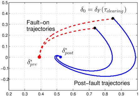
Figure 1: Convergence of the post-fault dynamics from two different fault-cleared states $\delta_{F}(\tau_{clearing}),$ which are obtained from two different fault-on dynamics at the clearing times $\tau_{clearing},$ to the post-fault equilibrium point $\delta^{*}_{post}.$

III-A Contingency Screening for Transient Stability

In contingency screening for transient stability, we consider three types of dynamics of power systems, namely pre-fault dynamics, fault-on dynamics and post-fault dynamics. In normal conditions, a power grid operates at a stable equilibrium point of the pre-fault dynamics. After the initial disturbance, the system evolves according to the fault-on dynamics laws and moves away from the pre-fault equilibrium point $\delta^{*}_{pre}$. After some time period, the fault is cleared or self-clears, and the system is at the fault-cleared state $\delta_{0}=\delta_{F}(\tau_{clearing})$. Then, the power system experiences the post-fault transient dynamics. The transient stability assessment problem addresses the question of whether the post-fault dynamics converges from the fault-cleared state to a post-fault stable equilibrium point $\delta^{*}_{post}$. Figure 1 shows the transient stability of the post-fault dynamics originated from the fault-cleared states to the stable post-fault equilibrium.

III-B Problem Formulation

The robust transient stability problem involves situations where there is uncertainty in power injections $P_{k},$ the sources of which are intermittent renewable generations and varying power consumptions. Particularly, while the parameters $m_{k},d_{k}$ are fixed and known, the power generations $P_{m_{k}}$ and load consumption $P^{0}_{d_{k}}$ are changing in time. As such, the post-fault equilibrium $\delta_{post}^{*}$ defined by (5) also variates. This raises the need for a robust stability certificate that can certify stability of post-fault dynamics with respect to a set of equilibria. When the power injections $P_{k}$ change in each transient stability assessment cycle, such a robust stability certificate can be repeatedly utilized in the “off-line” certification of system stability, eliminating the need for assessing stability on a regular basis. Formally, we consider the following robust stability problem:

• Robust stability w.r.t. a set of unknown equilibria: Given a fault-cleared state $\delta_{0},$ certify the transient stability of the post-fault dynamics described by (4) with respect to the set of stable equilibrium points $\Delta(\gamma)$.

We note that though the equilibrium point $\delta^{*}$ is unknown, we still can determine if it belongs to the set $\Delta(\gamma)$ by checking if the power injections satisfy the synchronization condition (6) or not.

The robust resiliency property denotes the ability of power systems to withstand a set of unknown disturbances and recover to the stable operating conditions. We consider the scenario where the disturbance results in line tripping. Then, it self-clears and the faulted line is reclosed. For simplicity, assume that the steady state power injections $P_{k}$ are unchanged during the fault-on dynamics. In that case, the pre-fault and post-fault equilibrium points defined by (5) are the same: $\delta_{pre}^{*}=\delta_{post}^{*}=\delta^{*}$ (this assumption is only for simplicity of presentation, we will discuss the case when $\delta_{pre}^{*}\neq\delta_{post}^{*}$). However, we assume that we don’t know which line is tripped/reclosed. Hence, there is a set of possible fault-on dynamics, and we want to certify if the power system can withstand this set of faults and recover to the stable condition $\delta^{*}$. Formally, this type of robust resiliency is formulated as follows.

• Robust resiliency w.r.t. a set of faults: Given a power system with the pre-fault and post-fault equilibrium point $\delta^{*}\in\Delta(\gamma),$ certify if the post-fault dynamics will return from any possible fault-cleared state $\delta_{0}$ to the equilibrium point $\delta^{*}$ regardless of the fault-on dynamics.

To resolve these problems in the next section, we utilize tools from nonlinear control theory. For this end, we separate the nonlinear couplings and the linear terminal system in (4). For brevity, we denote the stable post-fault equilibrium point for which we want to certify stability as $\delta^{*}.$ Consider the state vector $x=[x_{1},x_{2},x_{3}]^{T},$ which is composed of the vector of generator’s angle deviations from equilibrium $x_{1}=[\delta_{1}-\delta_{1}^{*},\dots,\delta_{|\mathcal{G}|}-\delta_{|\mathcal{G}|}^{*}]^{T}$, their angular velocities $x_{2}=[\dot{\delta}_{1},\dots,\dot{\delta}_{|\mathcal{G}|}]^{T}$, and vector of load buses’ angle deviation from equilibrium $x_{3}=[\delta_{{|\mathcal{G}|}+1}-\delta_{{|\mathcal{G}|}+1}^{*},\dots,\delta_{|\mathcal{N}|}-\delta_{|\mathcal{N}|}^{*}]^{T}$. Let $E$ be the incidence matrix of the graph $\mathcal{G}(\mathcal{N},\mathcal{E})$, so that $E[\delta_{1},\dots,\delta_{|\mathcal{N}|}]^{T}=[(\delta_{k}-\delta_{j})_{\{k,j\}\in\mathcal{E}}]^{T}$. Let the matrix $C$ be $E[I_{m\times m}\;O_{m\times n};O_{(n-m)\times 2m}\;I_{(n-m)\times(n-m)}].$ Then

$$Cx=E[\delta_{1}-\delta_{1}^{*},\dots,\delta_{|\mathcal{N}|}-\delta_{|\mathcal{N}|}^{*}]^{T}=[(\delta_{kj}-\delta_{kj}^{*})_{\{k,j\}\in\mathcal{E}}]^{T}.$$

Consider the vector of nonlinear interactions $F$ in the simple trigonometric form: $F(Cx)=[(\sin\delta_{kj}-\sin\delta^{*}_{kj})_{\{k,j\}\in\mathcal{E}}]^{T}.$ Denote the matrices of moment of inertia, frequency controller action on governor, and frequency coefficient of load as $M_{1}=\emph{\emph{diag}}(m_{1},\dots,m_{|\mathcal{G}|}),D_{1}=\emph{\emph{diag}}(d_{1},\dots,d_{|\mathcal{G}|})$ and $M=\emph{\emph{diag}}(m_{1},\dots,m_{|\mathcal{G}|},d_{|\mathcal{G}|+1},\dots,d_{|\mathcal{N}|}).$

In state space representation, the power system (4) can be then expressed in the following compact form:

$$\dot{x}_{1} =x_{2}$$

$$\dot{x}_{2} =M_{1}^{-1}D_{1}x_{2}-S_{1}M^{-1}E^{T}SF(Cx)$$ (7)

$$\dot{x}_{3} =-S_{2}M^{-1}E^{T}SF(Cx)$$

where $S=\emph{\emph{diag}}(a_{kj})_{\{k,j\}\in\mathcal{E}},S_{1}=[I_{m\times m}\quad O_{m\times n-m}],S_{2}=[O_{n-m\times m}\quad I_{n-m\times n-m}],n=|\mathcal{N}|,m=|\mathcal{G}|.$ Equivalently, we have

$$\dot{x}=Ax-BF(Cx),$$ (8)

with the matrices $A,B$ given by the following expression:

$$A=\left[\begin{array}[]{ccccc}O_{m\times m}&I_{m\times m}&O_{m\times n-m}\\ O_{m\times m}&-M_{1}^{-1}D_{1}&O_{m\times n-m}\\ O_{n-m\times m}&O_{n-m\times m}&O_{n-m\times n-m}\end{array}\right],$$

and

$$B=\left[\begin{array}[]{ccccc}O_{m\times|\mathcal{E}|};\quad S_{1}M^{-1}E^{T}S;\quad S_{2}M^{-1}E^{T}S\end{array}\right].$$

The key advantage of this state space representation of the system is the clear separation of nonlinear terms that are represented as a “diagonal” vector function composed of simple univariate functions applied to individual vector components. This feature will be exploited to construct Lyapunov functions for stability certificates in the next section.

IV Quadratic Lyapunov Function-based Stability and Resiliency Certificates

This section introduces the robust stability and resiliency certificates to address the problems (P1) and (P2) by utilizing quadratic Lyapunov functions. The construction of these quadratic Lyapunov functions is based on exploiting the strict bounds of the nonlinear vector $F$ in a region surrounding the equilibrium point and solving a linear matrix inequality (LMI). In comparison to the typically non-convex energy functions and Lur’e-Postnikov type Lyapunov functions, the convexity of quadratic Lyapunov functions enables the quick construction of the stability/resiliency certificates and the real-time stability assessment. Moreover, the certificates constructed in this work rely on the semi-local bounds of the nonlinear terms, which ensure that nonlinearity $F$ is linearly bounded in a polytope surrounding the equilibrium point. Therefore, though similar to the circle criterion, these stability certificates constitute an advancement to the classical circle criterion for stability in control theory where the nonlinearity is linearly bounded in the whole state space.

IV-A Strict Bounds for Nonlinear Couplings

The representation (8) of the structure-preserving model (4) with separation of nonlinear interactions allows us to naturally bound the nonlinearity of the system in the spirit of traditional approaches to nonlinear control [29, 30, 31]. Indeed, Figure 2 shows the natural bound of the nonlinear interactions $(\sin\delta_{kj}-\sin\delta_{kj}^{*})$ by the linear functions of angular difference $(\delta_{kj}-\delta_{kj}^{*})$. From Fig. 2, we observe that for all values of $\delta_{kj}=\delta_{k}-\delta_{j}$ such that $|\delta_{kj}|\leq\pi/2,$ we have:

$$g_{kj}(\delta_{kj}-\delta_{kj}^{*})^{2}\leq(\delta_{kj}-\delta_{kj}^{*})(\sin\delta_{kj}-\sin\delta_{kj}^{*})\leq(\delta_{kj}-\delta_{kj}^{*})^{2}$$ (9)

where

$$g_{kj}=\min\{\frac{1-\sin\delta_{kj}^{*}}{\pi/2-\delta_{kj}^{*}},\frac{1+\sin\delta_{kj}^{*}}{\pi/2+\delta_{kj}^{*}}\}=\frac{1-\sin|\delta_{kj}^{*}|}{\pi/2-|\delta_{kj}^{*}|}$$ (10)

As the function $(1-\sin t)/(\pi/2-t)$ is decreasing on $[0,\pi/2],$ it holds that

$$g_{kj}\geq\frac{1-\sin\lambda(\delta^{*})}{\pi/2-\lambda(\delta^{*})}:=g>0$$ (11)

where $\lambda(\delta^{*})$ is the maximum value of $|\delta_{kj}^{*}|$ over all the lines $\{k,j\}\in\mathcal{E},$ and $0\leq\lambda(\delta^{*})\leq\gamma<\pi/2.$ Therefore, in the polytope $\mathcal{P},$ defined by inequalities $|\delta_{kj}|\leq\pi/2,$ all the elements of the nonlinearities $F$ are bounded by:

$$g(\delta_{kj}-\delta_{kj}^{*})^{2}\leq(\delta_{kj}-\delta_{kj}^{*})(\sin\delta_{kj}-\sin\delta_{kj}^{*})\leq(\delta_{kj}-\delta_{kj}^{*})^{2}$$ (12)

and hence,

$$\big{(}F(Cx)-gCx\big{)}^{T}\big{(}F(Cx)-Cx\big{)}\leq 0,\forall x\in\mathcal{P}.$$ (13)

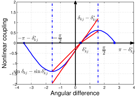
Figure 2: Strict bounds of nonlinear sinusoidal couplings $(\sin\delta_{kj}-\sin\delta^{*}_{kj})$ by two linear functions of the angular difference $\delta_{kj}$ as described in (12)

IV-B Quadratic Lyapunov Functions

In this section, we introduce the quadratic Lyapunov functions to analyze the stability of the general Lur’e-type system (8), which will be instrumental to the constructions of stability and resiliency certificates in this paper. The certificate construction is based on the following result which can be seen as an extension of the classical circle criterion to the case when the sector bound condition only holds in a finite region.

Lemma 1

Consider the general system in the form (8) in which the nonlinear vector $F$ satisfies the sector bound condition that $(F-K_{1}Cx)^{T}(F-K_{2}Cx)\leq 0$ for some matrices $K_{1},K_{2}$ and $x$ belonging to the set $\mathcal{S}.$ Assume that there exists a positive definite matrix $P$ such that

$$A^{T}P+PA-C^{T}K_{1}^{T}K_{2}C+R^{T}R\leq 0,$$ (14)

where $R=B^{T}P-\frac{1}{2}(K_{1}+K_{2})C.$ Then, the quadratic Lyapunov function $V(x(t))=x(t)^{T}Px(t)$ is decreasing along trajectory of the system (8) whenever $x(t)$ is in the set $\mathcal{S}$.

Proof: See Appendix VII-A. $\square$

Note that when $K_{1}=0$ or $K_{2}=0$ then Condition (14) leads to that the matrix $A$ have to be strictly stable. This condition does not hold for the case of structure-preserving model (4). Hence in case when $K_{1}=0$ or $K_{2}=0$, it is hard to have a quadratic Lyapunov function certifying the convergence of the system (4) by Lemma 1. Fortunately, when we restrict the system state $x$ inside the polytope $\mathcal{P}$ defined by inequalities $|\delta_{kj}|\leq\pi/2,$ we have strict bounds for the nonlinear interactions $F$ as in (12), in which $K_{1}=gI,K_{2}=I$ are strictly positive. Therefore, we can obtain the quadratic Lyapunov function certifying convergence of the structure-preserving model (4) as follows.

Lemma 2

Consider power grids described by the structure-preserving model (4) and satisfying Assumption 1. Assume that for given matrices $A,B,C,$ there exists a positive definite matrix $P$ of size $(|\mathcal{N}|+|\mathcal{G}|)$ such that

$$(A-\frac{1}{2}(1+g)BC)^{T}P+P(A-\frac{1}{2}(1+g)BC)$$

$$+PBB^{T}P+\frac{(1-g)^{2}}{4}C^{T}C\leq 0$$ (15)

or equivalently (by Schur complement) satisfying the LMI

$$\left[\begin{array}[]{cc}\bar{A}^{T}P+P\bar{A}+\dfrac{(1-g)^{2}}{4}C^{T}C&PB\\ B^{T}P&-I\\ \end{array}\right]\leq 0$$ (18)

where $\bar{A}=A-\dfrac{1}{2}(1+g)BC.$ Then, along (4), the Lyapunov function $V(x(t))$ is decreasing whenever $x(t)\in\mathcal{P}.$

Proof: From (12), we can see that the vector of nonlinear interactions $F$ satisfies the sector bound condition: $(F-K_{1}Cx)^{T}(F-K_{2}Cx)\leq 0,$ in which $K_{1}=gI,K_{2}=I$ and the set $\mathcal{S}$ is the polytope $\mathcal{P}$ defined by inequalities $|\delta_{kj}|\leq\pi/2.$ Applying Lemma 1, we have Lemma 2 straightforwardly. $\square$

We observe that the matrix $P$ obtained by solving the LMI (18) depends on matrices $A,B,C$ and the gain $g.$ Matrices $A,B,C$ do not depend on the parameters $P_{k}$ in the structure preserving model (4). Hence, we have a common triple of matrices $A,B,C$ for all the equilibrium point $\delta^{*}$ in the set $\Delta(\gamma).$ Also, whenever $\delta^{*}\in\Delta(\gamma)$, we can replace $g$ in (11) by the lower bound of $g$ as $g=\dfrac{1-\sin\gamma}{\pi/2-\gamma}>0.$ This lower bound also does not depend on the equilibrium point $\delta^{*}$ at all. Then, the matrix $P$ is independent of the set $\Delta(\gamma)$ of stable equilibrium points $\delta^{*}.$ Therefore, Lemma 2 provides us with a common quadratic Lyapunov function for any post-fault dynamics with post-fault equilibrium point $\delta^{*}\in\Delta(\gamma)$. In the next section, we present the transient stability certificate based on this quadratic Lyapunov function.

IV-C Transient Stability Certificate

Before proceeding to robust stability/resiliency certificates in the next sections, we will present the transient stability certificate. We note that the Lyapunov function $V(x)$ considered in Lemma 2 is decreasing whenever the system trajectory evolves inside the polytope $\mathcal{P}.$ Outside $\mathcal{P},$ the Lyapunov function is possible to increase. In the following, we will construct inside the polytope $\mathcal{P}$ an invariant set $\mathcal{R}$ of the post-fault dynamics described by structure-preserving system (4). Then, from any point inside this invariant set $\mathcal{R}$, the post-fault dynamics (4) will only evolve inside $\mathcal{R}$ and eventually converge to the equilibrium point due to the decrease of the Lyapunov function $V(x)$.

Indeed, for each edge $\{k,j\}$ connecting the generator buses $k$ and $j,$ we divide the boundary $\partial\mathcal{P}_{kj}$ of $\mathcal{P}$ corresponding to the equality $|\delta_{kj}|=\pi/2$ into two subsets $\partial\mathcal{P}_{kj}^{in}$ and $\partial\mathcal{P}_{kj}^{out}$. The flow-in boundary segment $\partial\mathcal{P}_{kj}^{in}$ is defined by $|\delta_{kj}|=\pi/2$ and $\delta_{kj}\dot{\delta}_{kj}<0,$ while the flow-out boundary segment $\partial\mathcal{P}_{kj}^{out}$ is defined by $|\delta_{kj}|=\pi/2$ and $\delta_{kj}\dot{\delta}_{kj}\geq 0.$ Since the derivative of $\delta_{kj}^{2}$ at every points on $\partial\mathcal{P}_{kj}^{in}$ is negative, the system trajectory of (4) can only go inside $\mathcal{P}$ once it meets $\partial\mathcal{P}_{kj}^{in}.$

Define the following minimum value of the Lyapunov function $V(x)$ over the flow-out boundary $\partial\mathcal{P}^{out}$ as:

$$V_{\min}=\mathop{\min}\limits_{x\in\partial\mathcal{P}^{out}}V(x),$$ (19)

where $\partial\mathcal{P}^{out}$ is the flow-out boundary of the polytope $\mathcal{P}$ that is the union of $\partial\mathcal{P}_{kj}^{out}$ over all the transmission lines $\{k,j\}\in\mathcal{E}$ connecting generator buses. From the decrease of $V(x)$ inside the polytope $\mathcal{P},$ we can have the following center result regarding transient stability assessment.

Theorem 1

For a post-fault equilibrium point $\delta^{*}\in\Delta(\gamma)$, from any initial state $x_{0}$ staying in set $\mathcal{R}$ defined by

$$\mathcal{R}=\{x\in\mathcal{P}:V(x)<V_{\min}\},$$ (20)

then, the system trajectory of (4) will only evolve in the set $\mathcal{R}$ and eventually converge to the stable equilibrium point $\delta^{*}.$

Proof: See Appendix VII-B. $\square$

Remark 1

Since the Lyapunov function $V(x)$ is convex, finding the minimum value $V_{\min}=\min_{x\in\partial\mathcal{P}^{out}}V(x)$ can be extremely fast. Actually, we can have analytical form of $V_{\min}.$ This fact together with the LMI-based construction of the Lyapunov function $V(x)$ allows us to perform the transient stability assessment in the real time.

Remark 2

Theorem 1 provides a certificate to determine if the post-fault dynamics will evolve from the fault-cleared state $x_{0}$ to the equilibrium point. By this certificate, if $x_{0}\in\mathcal{R},$ i.e. if $x_{0}\in\mathcal{P}$ and $V(x_{0})<V_{\min}$, then we are sure that the post-fault dynamics is stable. If this is not true, then there is no conclusion for the stability or instability of the post-fault dynamics by this certificate.

Remark 3

The transient stability certificate in Theorem 1 is effective to assess the transient stability of post-fault dynamics where the fault-cleared state is inside the polytope $\mathcal{P}.$ It can be observed that the polytope $\mathcal{P}$ contains almost all practically interesting configurations. In real power grids, high differences in voltage phasor angles typically result in triggering of protective relay equipment and make the dynamics of the system more complicated. Contingencies that trigger those events are rare but potentially extremely dangerous. They should be analyzed individually with more detailed and realistic models via time-domain simulations.

Remark 4

The stability certificate in Theorem 1 is constructed similarly to that in [16]. The main feature distinguishing the certificate in Theorem 1 is that it is based on the quadratic Lyapunov function, instead of the Lur’e-Postnikov type Lyapunov function as in [16]. As such, we can have an analytical form for $V_{\min}$ rather than determining it by a potentially non-convex optimization as in [16].

IV-D Robust Stability w.r.t. Power Injection Variations

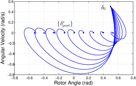
Figure 3: Robust transient stability of the post-fault dynamics originated from the fault-cleared state $\delta_{0}=[0.5\;\;0.5]^{T}$ to the set of stable equilibrium points $\Delta(\pi/6)=\{\delta_{post}^{*}=[\delta^{*},0]^{T}:-\pi/6\leq\delta^{*}\leq\pi/6\}.$

In this section, we develop a “robust” extension of the stability certificate in Theorem 1 that can be used to assess transient stability of the post-fault dynamics described by the structure-preserving model (4) in the presence of power injection variations. Specifically, we consider the system whose stable equilibrium point variates but belongs to the set $\Delta(\gamma).$ As such, whenever the power injections $P_{k}$ satisfy the synchronization condition (6), we can apply this robust stability certificate without exactly knowing the equilibrium point of the system (4).

As discussed in Remark 3, we are only interested in the case when the fault-cleared state is in the polytope $\mathcal{P}.$ Denote $\delta=[\delta_{1},...,\delta_{|\mathcal{G}|},\dot{\delta}_{1},...,\dot{\delta}_{|\mathcal{G}|},\delta_{|\mathcal{G}|+1},...,\delta_{|\mathcal{N}|}].$ The system state $x$ and the fault-cleared state $x_{0}$ can be then presented as $x=\delta-\delta^{*}$ and $x_{0}=\delta_{0}-\delta^{*}.$ Exploiting the independence of the LMI (18) on the equilibrium point $\delta^{*},$ we have the following robust stability certificate for the problem (P1).

Theorem 2

Consider the post-fault dynamics (4) with uncertain stable equilibrium point $\delta^{*}$ that satisfies $\delta^{*}\in\Delta(\gamma).$ Consider a fault-cleared state $\delta_{0}\in\mathcal{P},$ i.e., $|\delta_{0_{kj}}|\leq\pi/2,\forall\{k,j\}\in\mathcal{E}.$ Suppose that there exists a positive definite matrix $P$ of size $(|\mathcal{N}|+|\mathcal{G}|)$ satisfying the LMI (18) and

$$\delta_{0}^{T}P\delta_{0}<\min_{\delta\in\partial\mathcal{P}^{out},\delta^{*}\in\Delta(\gamma)}\big{(}\delta^{T}P\delta-2{\delta^{*}}^{T}P(\delta-\delta_{0})\big{)}$$ (21)

Then, the system (4) will converge from the fault-cleared state $\delta_{0}$ to the equilibrium point $\delta^{*}$ for any $\delta^{*}\in\Delta(\gamma).$

Proof: See Appendix VII-C. $\square$

Remark 5

Theorem 2 gives us a robust certificate to assess the transient stability of the post-fault dynamics (4) in which the power injections $P_{k}$ variates. First, we check the synchronization condition (6), the satisfaction of which tells us that the equilibrium point $\delta^{*}$ is in the set $\Delta(\gamma).$ Second, we calculate the positive definite matrix $P$ by solving the LMI (18) where the gain $g$ is defined as $(1-\sin\gamma)/(\pi/2-\gamma).$ Lastly, for a given fault-cleared state $\delta_{0}$ staying inside the polytope $\mathcal{P},$ we check whether the inequality (21) is satisfied or not. In the former case, we conclude that the post-fault dynamics (4) will converge from the fault-cleared state $\delta_{0}$ to the equilibrium point $\delta^{*}$ regardless of the variations in power injections. Otherwise, we repeat the second step to find other positive definite matrix $P$ and check the condition (21) again.

Remark 6

Note that there are possibly many matrices $P$ satisfying the LMI (18). This gives us flexibility in choosing $P$ satisfying both (18) and (21) for a given fault-cleared state $\delta_{0}$. A heuristic algorithm as in [16] can be used to find the best suitable matrix $P$ in the family of such matrices defined by (18) for the given fault-cleared state $\delta_{0}$ after a finite number of steps.

Remark 7

In practice, to reduce the conservativeness and computational time in the assessment process, we can off-line compute the common matrix $P$ for any equilibrium point $\delta^{*}\in\Delta(\gamma)$ and check on-line the condition $V(x_{0})<V_{\min}$ with the data (initial state $x_{0}$ and power injections $P_{k}$) obtained on-line. In some case the initial state can be predicted before hand, and if there exists a positive definite matrix $P$ satisfying the LMI (18) and the inequality (21), then the on-line assessment is reduced to just checking condition (6) for the power injections $P_{k}.$

IV-E Robust Resiliency w.r.t. a Set of Faults

In this section, we introduce the robust resiliency certificate with respect to a set of faults to solve the problem (P2). We consider the case when the fault results in tripping of a line. Then it self-clears and the line is reclosed. But we don’t know which line is tripped/reclosed. Note that the pre-fault equilibrium and post-fault equilibrium, which are obtained by solving the power flow equations (5), are the same and given.

With the considered set of faults, we have a set of corresponding fault-on dynamic flows, which drive the system from the pre-fault equilibrium point to a set of fault-cleared states at the clearing time. We will introduce technique to bound the fault-on dynamics, by which we can bound the set of reachable fault-cleared states. With this way, we make sure that the reachable set of fault-cleared states remain in the region of attraction of the post-fault equilibrium point, and thus the post-fault dynamics is stable.

Indeed, we first introduce the resiliency certificate for one fault associating with one faulted transmission line, and then extend it to the robust resiliency certificate for any faulted line. With the fault of tripping the transmission line $\{u,v\}\in\mathcal{E}$, the corresponding fault-on dynamics can be obtained from the structure-preserving model (4) after eliminating the nonlinear interaction $a_{uv}\sin\delta_{uv}.$ Formally, the fault-on dynamics is described by

$$\dot{x}_{F}=Ax_{F}-BF(Cx_{F})+BD_{\{u,v\}}\sin\delta_{F_{uv}},$$ (22)

where $D_{\{u,v\}}$ is the unit vector to extract the $\{u,v\}$ element from the vector of nonlinear interactions $F.$ Here, we denote the fault-on trajectory as $x_{F}(t)$ to differentiate it from the post-fault trajectory $x(t).$ We have the following resiliency certificate for the power system with equilibrium point $\delta^{*}$ subject to the faulted-line $\{u,v\}$ in the set $\mathcal{E}$.

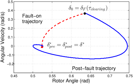
Figure 4: Robust resiliency of power system with respect to the faults whenever the clearing time $\tau_{clearing}<\mu V_{\min}.$

Theorem 3

Assume that there exist a positive definite matrix $P$ of size $(|\mathcal{N}|+|\mathcal{G}|)$ and a positive number $\mu$ such that

$$\bar{A}^{T}P+P\bar{A}+\dfrac{(1-g)^{2}}{4}C^{T}C$$

$$+PBB^{T}P+\mu PBD_{\{u,v\}}D_{\{u,v\}}^{T}B^{T}P\leq 0.$$ (23)

Assume that the clearing time $\tau_{clearing}$ satisfies $\tau_{clearing}<\mu V_{\min}$ where $V_{\min}=\min_{x\in\partial\mathcal{P}^{out}}V(x)$. Then, the fault-cleared state $x_{F}(\tau_{clearing})$ resulted from the fault-on dynamics (22) is still inside the region of attraction of the post-fault equilibrium point $\delta^{*}$, and the post-fault dynamics following the tripping and reclosing of the line $\{u,v\}$ returns to the original stable operating condition.

Proof: See Appendix VII-D.

Remark 8

Note that the inequality (3) can be rewritten as

$$\bar{A}^{T}P+P\bar{A}+\dfrac{(1-g)^{2}}{4}C^{T}C+P\bar{B}\bar{B}^{T}P\leq 0,$$ (24)

where $\bar{B}=[B\;\;\sqrt{\mu}BD_{\{u,v\}}].$ By Schur complement, inequality (24) is equivalent with

$$\left[\begin{array}[]{cc}\bar{A}^{T}P+P\bar{A}+\dfrac{(1-g)^{2}}{4}C^{T}C&P\bar{B}\\ \bar{B}^{T}P&-I\\ \end{array}\right]\leq 0.$$ (27)

With a fixed value of $\mu$, the inequality (27) is an LMI which can be transformed to a convex optimization problem. As such, the inequality (3) can be solved quickly by a heuristic algorithm in which we vary $\mu$ and find $P$ accordingly from the LMI (27) with fixed $\mu$. Another heuristic algorithm to solve the inequality (3) is to solve the LMI (18), and for each solution $P$ in this family of solutions, find the maximum value of $\mu$ such that (3) is satisfied.

Remark 9

For the case when the pre-fault and post-fault equilibrium points are different, Theorem 3 still holds true if we replace the condition $\tau_{clearing}<\mu V_{\min}$ by condition $\tau_{clearing}<\mu\big{(}V_{\min}-V(x_{pre})\big{)},$ where $x_{pre}=\delta^{*}_{pre}-\delta^{*}_{post}.$

Remark 10

The resiliency certificate in Theorem 3 is straightforward to extend to a robust resiliency certificate with respect to the set of faults causing tripping and reclosing of transmission lines in the grids. Indeed, we will find the positive definite matrix $P$ and positive number $\mu$ such that the inequality (3) is satisfied for all the matrices $D_{\{u,v\}}$ corresponding to the faulted line $\{u,v\}\in\mathcal{E}.$ Let $D$ be a matrix larger than or equals to the matrices $D_{\{u,v\}}D_{\{u,v\}}^{T}$ for all the transmission lines in $\mathcal{E}$ (here, that $X$ is larger than or equals to $Y$ means that $X-Y$ is positive semidefinite). Then, any positive definite matrix $P$ and positive number $\mu$ satisfying the inequality (3), in which the matrix $D_{\{u,v\}}D_{\{u,v\}}^{T}$ is replaced by $D,$ will give us a quadratic Lyapunov function-based robust stability certificate with respect to the set of faults similar to Theorem 3. Since $D_{\{u,v\}}D_{\{u,v\}}^{T}=\emph{\emph{diag}}(0,\dots,1,\dots,0)$ are orthogonal unit matrices, we can see that the probably best matrix we can have is $D=\sum_{\{u,v\}\in\mathcal{E}}D_{\{u,v\}}D_{\{u,v\}}^{T}=I_{|\mathcal{E}|\times|\mathcal{E}|}.$ Accordingly, we have the following robust resilience certificate for any faulted line happening in the system.

Theorem 4

Assume that there exist a positive definite matrix $P$ of size $(|\mathcal{N}|+|\mathcal{G}|)$ and a positive number $\mu$ such that

$$\bar{A}^{T}P+P\bar{A}+\dfrac{(1-g)^{2}}{4}C^{T}C+(1+\mu)PBB^{T}P\leq 0.$$ (28)

Assume that the clearing time $\tau_{clearing}$ satisfies $\tau_{clearing}<\mu V_{\min}$ where $V_{\min}=\min_{x\in\partial\mathcal{P}^{out}}V(x)$. Then, for any faulted line happening in the system the fault-cleared state $x_{F}(\tau_{clearing})$ is still inside the region of attraction of the post-fault equilibrium point $\delta^{*}$, and the post-fault dynamics returns to the original stable operating condition regardless of the fault-on dynamics.

Remark 11

By the robust resiliency certificate in Theorem 4, we can certify stability of power system with respect to any faulted line happens in the system. This certificate as well as the certificate in Theorem 3 totally eliminates the needs for simulations of the fault-on dynamics, which is currently indispensable in any existing contingency screening methods for transient stability.

V Numerical Illustrations

V-A 2-Bus System

For illustration purpose, this section presents the simulation results on the most simple 2-bus power system, described by the single 2-nd order differential equation

$$m\ddot{\delta}+d\dot{\delta}+a\sin\delta-p=0.$$ (29)

For numerical simulations, we choose $m=0.1$ p.u., $d=0.15$ p.u., $a=0.2$ p.u. When the parameters $p$ changes from $-0.1$ p.u. to $0.1$ p.u., the stable equilibrium point $\delta^{*}$ (i.e. $[\delta^{*}\;0]^{T}$) of the system belongs to the set: $\Delta=\{\delta^{*}:|\delta^{*}|\leq\arcsin(0.1/0.2)=\pi/6\}.$ For the given fault-cleared state $\delta_{0}=[0.5\;\;0.5],$ using the CVX software we obtain a positive matrix $P$ satisfying the LMI (18) and the condition for robust stability (21) as $P=[0.8228\;\;0.1402;0.1402\;\;0.5797].$ The simulations confirm this result. We can see in Fig. 3 that from the fault-cleared state $\delta_{0}$ the post-fault trajectory always converges to the equilibrium point $\delta^{*}$ for all $\delta^{*}\in\Delta(\pi/6).$ Figure 5 shows the convergence of the quadratic Lyapunov function to $0.$

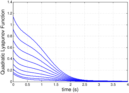
Figure 5: Convergence of the quadratic Lyapunov function $V(x)=x^{T}Px=(\delta-\delta^{*})^{T}P(\delta-\delta^{*})$ from the initial value to $0$ when the equilibrium point $\delta^{*}$ varies in the set $\Delta(\pi/6)=\{\delta_{post}^{*}=[\delta^{*},0]^{T}:-\pi/6\leq\delta^{*}\leq\pi/6\}.$

Now we consider the resiliency certificate in Theorem 3 with respect to fault of tripping the line and self-clearing. The pre-fault and post-fault dynamics have the fixed equilibrium point: $\delta^{*}=[\pi/6\;0]^{T}.$ Then the positive definite matrix $P=[0.0822\;\;0.0370;0.0370\;\;0.0603]$ and positive number $\mu=6$ is a solution of the inequality (3). As such, for any clearing time $\tau_{clearing}<\mu V_{min}=0.5406,$ the fault-cleared state is still in the region of attraction of $\delta^{*},$ and the power system withstands the fault. Figure 4 confirms this prediction. Figure 6 shows that during the fault-on dynamics, the Lyapunov function is strictly increasing. After the clearing time $\tau_{clearing},$ the Lyapunov function decreases to $0$ as the post-fault trajectory converges to the equilibrium point $\delta^{*}.$

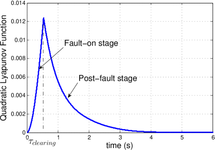
Figure 6: Variations of the quadratic Lyapunov function $V(x)=x^{T}Px=(\delta-\delta^{*})^{T}P(\delta-\delta^{*})$ during the fault-on and post-fault dynamics.

V-B Robust Resiliency Certificate for 3-Generator System

To illustrate the effectiveness of the robust resiliency certificate in Theorem 4, we consider the system of three generators with the time-invariant terminal voltages and mechanical torques given in Tab. I.

Node	V (p.u.)	P (p.u.)
1	1.0566	-0.2464
2	1.0502	0.2086
3	1.0170	0.0378

TABLE I: Voltage and mechanical input

The susceptance of the transmission lines are $B_{12}=0.739$ p.u., $B_{13}=1.0958$ p.u., and $B_{23}=1.245$ p.u. The equilibrium point is calculated from (5): $\delta^{*}=[-0.6634\;-0.5046\;-0.5640\;0\;0\;0]^{T}.$ By using CVX software we can find one solution of the inequality (28) as $\mu=0.3$ and the positive definite matrix $P$ as

$$\left[\begin{array}[]{cccccc}2.4376&1.7501&1.8190&4.0789&3.9566&3.9780\\ 1.7501&2.3991&1.8576&3.9639&4.0710&3.9785\\ 1.8190&1.8576&2.3302&3.9707&3.9859&4.0569\\ 4.0789&3.9639&3.9707&17.2977&16.6333&16.7452\\ 3.9566&4.0710&3.9859&16.6333&17.2425&16.8003\\ 3.9780&3.9785&4.0569&16.7452&16.8003&17.1306\\ \end{array}\right]$$

The corresponding minimum value of Lyapunov function is $V_{\min}=0.5536.$ Hence, for any faults resulting in tripping and reclosing lines in $\mathcal{E},$ whenever the clearing time less than $\mu V_{\min}=0.1661,$ then the power system still withstands all the faults and recovers to the stable operating condition at $\delta^{*}.$

V-C 118 Bus System

Our test system in this section is the modified IEEE 118-bus test case [32], of which 54 are generator buses and the other 64 are load buses as showed in Fig. 7. The data is taken directly from the test files [32], otherwise specified. The damping and inertia are not given in the test files and thus are randomly selected in the following ranges: $m_{i}\in[2,4],\forall i\in\mathcal{G},$ and $d_{i}\in[1,2],\forall i\in\mathcal{N}.$ The grid originally contains 186 transmission lines. We eliminate 9 lines whose susceptance is zero, and combine 7 lines $\{42,49\},\{49,54\},\{56,59\},\{49,66\},\{77,80\},$ $\{89,90\},$ and $\{89,92\},$ each of which contains double transmission lines as in the test files [32]. Hence, the grid is reduced to 170 transmission lines connecting 118 buses. We renumber the generator buses as $1-54$ and load buses as $55-118$.

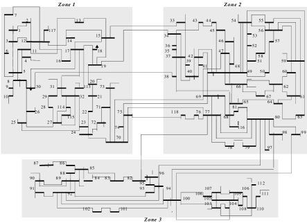
Figure 7: IEEE 118-bus test case

1) Stability Assessment

We assume that there are varying generations (possibly due to renewable) at 16 buses $1-16$ (i.e. $30\%$ generator buses are varying). The system is initially at the equilibrium point given in [32], but the variations in the renewable generations make the operating condition to change. We want to assess if the system will transiently evolve from the initial state to the new equilibrium points. To make our proposed robust stability assessment framework valid, we assume that the renewable generators have the similar dynamics with the conventional generator but with the varying power output. This happens when we equip renewable generators with synchronverter [33], which will control the dynamics of renewables to mimic the dynamics of conventional generators. Using the CVX software with Mosek solver, we can see that there exists positive definite matrix $P$ satisfying the LMI (18) and the inequality (21) with $\gamma=\pi/12.$ As such, the grid will transiently evolve from the initial state to any new equilibrium point in the set $\Delta(\pi/12).$ To demonstrate this result by simulation, we assume that in the time period $[20s,30s],$ the power outputs of the renewable generators increase $50\%.$ Since the synchronization condition $\|L^{{\dagger}}p\|_{\mathcal{E},\infty}=0.1039<\sin(\pi/12)$ holds true, we can conclude that the new equilibrium point, obtained when the renewable generations increased $50\%,$ will stay in the set $\Delta(\pi/12).$ From Fig. 8, we can see that the grid transits from the old equilibrium point to the new equilibrium point when the renewable power outputs increase. Similarly, if in the time period $[20s,30s]$ the power outputs of the renewable generators decrease $50\%,$ then we can check that $\|L^{{\dagger}}p\|_{\mathcal{E},\infty}=0.0762<\sin(\pi/12)$. Therefore by the robust stability certificate, we conclude that the grid evolves from the old equilibrium point to the new equilibrium point, as confirmed in Fig. 9.

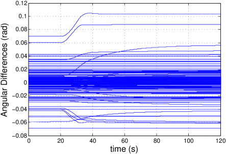
Figure 8: Transition of the 118-bus system from the old equilibrium to the new equilibrium when the renewable generations increase $50\%$ in the period $[20s,30s]$

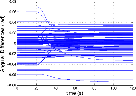
Figure 9: Transition of the 118-bus system from the old equilibrium to the new equilibrium when the renewable generations decrease $50\%$ in the period $[20s,30s]$

2) Resiliency Assessment We note that in many cases in practice, when the fault causes tripping one line, we end up with a new power system with a stable equilibrium point possibly staying inside the small polytope $\Delta(\gamma).$ As such, using the robust stability assessment in the previous section we can certify that, if the fault is permanent, then the system will transit from the old equilibrium point to the new equilibrium point. Therefore, to demonstrate the resiliency certificate we do not need to consider all the tripped lines, but only concern the case when tripping a critical line may result in an unstable dynamics, and we use the resiliency assessment framework to determine if the clearing time is small enough such that the post-fault dynamics recovers to the old equilibrium point.

Consider such a critical case when the transmission line connecting the generator buses 19 and 21 is tripped. It can be checked that in this case the synchronization condition (6) is not satisfied even with $\gamma\approx\pi/2$ since $\|L^{{\dagger}}p\|_{\mathcal{E},\infty}=1.5963>\sin(\pi/2).$ As such, we cannot make sure that the fault-on dynamics caused by tripping the transmission line $\{19,21\}$ will converge to a stable equilibrium point in the set $\Delta(\pi/2)$. Now assume that the fault self-clears and the transmission line $\{19,21\}$ is reclosed at the clearing time $\tau_{clearing}$. With $\mu=0.11$ and using CVX software with Mosek solver on a laptop (Intel-core i5 2.6GHz, 8GB RAM), it takes $1172s$ to find a positive definite matrix $P$ satisfying the inequality (27) and to calculate the corresponding minimum value of Lyapunov function as $V_{\min}$=0.927. As such, whenever the clearing time satisfies $\tau_{clearing}<\mu V_{\min}=0.102s$, then the fault-cleared state is still inside the region of attraction of the post-fault equilibrium point, i.e. the power system withstands the tripping of critical line and recover to its stable operating condition.

VI Conclusions and Path Forward

This paper has formulated two novel robust stability and resiliency problems for nonlinear power grids. The first problem is the transient stability of a given fault-cleared state with respect to a set of varying post-fault equilibrium points, particularly applicable to power systems with varying power injections. The second one is the resiliency of power systems subject to a set of unknown faults, which result in line tripping and then self-clearing. These robust stability and resiliency certificates can help system operators screen multiple contingencies and multiple power injection profiles, without relying on computationally wasteful real-time simulations. Exploiting the strict bounds of nonlinear power flows in a practically relevant polytope surrounding the equilibrium point, we introduced the quadratic Lyapunov functions approach to the constructions of these robust stability/resiliency certificates. The convexity of quadratic Lyapunov functions allowed us to perform the stability assessment in the real time.

There are many directions can be pursued to push the introduced robust stability/resiliency certificates to the industrially ready level. First, and most important, the algorithms should be extended to more general higher order models of generators [34]. Although these models can be expected to be weakly nonlinear in the vicinity of an equilibrium point, the higher order model systems are no longer of Lur’e type and have multi-variate nonlinear terms. It is necessary to extend the construction from sector-bounded nonlinearities to more general norm-bounded nonlinearities [35].

It is also promising to extend the approaches described in this paper to a number of other problems of high interest to power system community. These problems include intentional islanding [36], where the goal is to identify the set of tripping signals that can stabilize the otherwise unstable power system dynamics during cascading failures. This problem is also interesting in a more general context of designing and programming of the so-called special protection system that help to stabilize the system with the control actions produced by fast power electronics based HVDC lines and FACTS devices. Finally, the introduced certificates of transient stability can be naturally incorporated in operational and planning optimization procedures and eventually help in development of stability-constrained optimal power flow and unit commitment approaches [37, 38].

VII Appendix

VII-A Proof of Lemma 1

Along the trajectory of (8), we have

$$\dot{V}(x)=\dot{x}^{T}Px+x^{T}P\dot{x}=x^{T}(A^{T}P+PA)x-2x^{T}PBF$$ (30)

Let $W(x)=(F-K_{1}Cx)^{T}(F-K_{2}Cx).$ Then, $W(x)\leq 0,\forall x\in\mathcal{S}$ and $W(x)=F^{T}F-F^{T}(K_{1}+K_{2})Cx+x^{T}C^{T}K_{1}^{T}K_{2}Cx.$ Subtracting $W$ from $\dot{V}(x),$ we obtain:

$$\dot{V}(x)-W(x)=x^{T}(A^{T}P+PA)x-2x^{T}PBF$$

$$-F^{T}F+F^{T}(K_{1}+K_{2})Cx-x^{T}C^{T}K_{1}^{T}K_{2}Cx$$

$$=x^{T}(A^{T}P+PA)x-x^{T}C^{T}K_{1}^{T}K_{2}Cx$$

$$-\big{\|}F+(B^{T}P-\frac{(K_{1}+K_{2})C}{2})x\big{\|}^{2}$$

$$+x^{T}\big{[}B^{T}P-\frac{(K_{1}+K_{2})C}{2}\big{]}^{T}\big{[}B^{T}P-\frac{(K_{1}+K_{2})C}{2}\big{]}x$$

$$=x^{T}\big{[}A^{T}P+PA-C^{T}K_{1}^{T}K_{2}C+R^{T}R\big{]}x-S^{T}S,$$ (31)

where $R=B^{T}P-\frac{1}{2}(K_{1}+K_{2})C$ and $S=F+(B^{T}P-\frac{1}{2}(K_{1}+K_{2})C)x.$

Note that (14) is equivalent with the existence of a non-negative matrix $Q$ such that

$$A^{T}P+PA-C^{T}K_{1}^{T}K_{2}C+R^{T}R=-Q$$ (32)

Therefore:

$$\dot{V}(x)=W(x)-x^{T}Qx-S^{T}S\leq 0,\forall x\in\mathcal{S}$$ (33)

As such $V(x(t))$ is decreasing along trajectory $x(t)$ of (8) whenever $x(t)$ is in the set $\mathcal{S}.$ $\square$

VII-B Proof of Theorem 1

The boundary of the set $\mathcal{R}$ defined as in (20) is composed of segments which belong to the boundary of the polytope $\mathcal{P}$ and segments which belong to the Lyapunov function’s sublevel set. Due to the decrease of $V(x)$ in the polytope $\mathcal{P}$ and the definition of $V_{\min},$ the system trajectory of (4) cannot escape the set $\mathcal{R}$ through the flow-out boundary and the sublevel-set boundary. Also, once the system trajectory of (4) meets the flow-in boundary, it will go back inside $\mathcal{R}.$ Therefore, the system trajectory of (4) cannot escape $\mathcal{R},$ i.e. $\mathcal{R}$ is an invariant set of (4).

Since $\mathcal{R}$ is a subset of the polytope $\mathcal{P},$ from Lemma 2 we have $\dot{V}(x(t))\leq 0$ for all $t\geq 0.$ By LaSalle’s Invariance Principle, we conclude that the system trajectory of (4) will converge to the set $\{x\in\mathcal{P}:\dot{V}(x)=0\},$ which together with (33) means that the system trajectory of (4) will converge to the equilibrium point $\delta^{*}$ or to some stationary points lying on the boundary of $\mathcal{P}.$ From the decrease of $V(x)$ in the polytope $\mathcal{P}$ and the definition of $V_{\min},$ we can see that the second case cannot happen. Therefore, the system trajectory will converge to the equilibrium point $\delta^{*}.$ $\square$

VII-C Proof of Theorem 2

Since the matrix $P,$ the polytope $\mathcal{P},$ and the fault-cleared state $\delta_{0}$ are independent of the equilibrium point $\delta^{*},$ we have

$$V_{\min}-V(x_{0}) =\mathop{\min}\limits_{x\in\partial\mathcal{P}^{out}}\big{(}(\delta-\delta^{*})^{T}P(\delta-\delta^{*})$$

$$\qquad\qquad\quad-(\delta_{0}-\delta^{*})^{T}P(\delta_{0}-\delta^{*})\big{)}$$

$$=\mathop{\min}\limits_{\delta\in\partial\mathcal{P}^{out}}(\delta^{T}P\delta-\delta_{0}^{T}P\delta_{0}-2{\delta^{*}}^{T}P(\delta-\delta_{0}))$$

$$=\mathop{\min}\limits_{\delta\in\partial\mathcal{P}^{out}}(\delta^{T}P\delta-2{\delta^{*}}^{T}P(\delta-\delta_{0}))-\delta_{0}^{T}P\delta_{0}$$ (34)

Hence, if $\mathop{\min}\limits_{\delta\in\partial\mathcal{P}^{out},\delta^{*}\in\Delta(\gamma)}(\delta^{T}P\delta-2{\delta^{*}}^{T}P(\delta-\delta_{0}))>\delta_{0}^{T}P\delta_{0},$ then $V_{\min}>V(x_{0})$ for all $\delta^{*}\in\Delta(\gamma).$ Applying Theorem 1, we have Theorem 2 directly. $\square$

VII-D Proof of Theorem 3

Similar to the proof of Lemma 1, we have the derivative of $V(x)$ along the fault-on trajectory (22) as follows:

$$\dot{V}(x_{F}) =\dot{x_{F}}^{T}Px_{F}+x_{F}^{T}P\dot{x_{F}}=x_{F}^{T}(A^{T}P+PA)x_{F}$$

$$-2x_{F}^{T}PBF+2x_{F}^{T}PBD_{\{u,v\}}\sin\delta_{F_{uv}}$$

$$=W(x_{F})-S^{T}S+2x_{F}^{T}PBD_{uv}\sin\delta_{F_{uv}}$$

$$+x_{F}^{T}\big{[}A^{T}P+PA-C^{T}K_{1}^{T}K_{2}C+R^{T}R\big{]}x_{F}$$ (35)

On the other hand

$$2x_{F}^{T}PBD_{\{u,v\}}\sin\delta_{F_{uv}} \leq\mu x_{F}^{T}PBD_{\{u,v\}}D_{\{u,v\}}^{T}B^{T}Px_{F}$$

$$+\dfrac{1}{\mu}\sin^{2}\delta_{F_{uv}}.$$ (36)

Therefore,

$$\dot{V}(x_{F})\leq W(x_{F})-S^{T}S+x_{F}^{T}\tilde{Q}x_{F}+\frac{1}{\mu}\sin^{2}\delta_{F_{uv}}$$ (37)

where $\tilde{Q}=A^{T}P+PA-C^{T}K_{1}^{T}K_{2}C+R^{T}R+\mu PBD_{\{u,v\}}D_{\{u,v\}}^{T}B^{T}P$. Note that $W(x_{F})\leq 0,\forall x_{F}\in\mathcal{P},$ and

$$\tilde{Q} =\bar{A}^{T}P+P\bar{A}+\dfrac{(1-g)^{2}}{4}C^{T}C$$

$$+PBB^{T}P+\mu PBD_{\{u,v\}}D_{\{u,v\}}^{T}B^{T}P\leq 0.$$ (38)

Therefore,

$$\dot{V}(x_{F})\leq\frac{1}{\mu}\sin^{2}\delta_{F_{uv}}\leq\frac{1}{\mu},$$ (39)

whener $x_{F}$ in the polytope $\mathcal{P}.$

We will prove that the fault-cleared state $x_{F}(\tau_{clearing})$ is still in the set $\mathcal{R}.$ It is easy to see that the flow-in boundary $\partial\mathcal{P}^{in}$ prevents the fault-on dynamics (22) from escaping $\mathcal{R}.$

Assume that $x_{F}(\tau_{clearing})$ is not in the set $\mathcal{R}.$ Then the fault-on trajectory can only escape $\mathcal{R}$ through the segments which belong to sublevel set of the Lyapunov function $V(x).$ Denote $\tau$ be the first time at which the fault-on trajectory meets one of the boundary segments which belong to sublevel set of the Lyapunov function $V(x).$ Hence $x_{F}(t)\in\mathcal{R}$ for all $0\leq t\leq\tau.$ From (39) and the fact that $\mathcal{R}\subset\mathcal{P},$ we have

$$V(x_{F}(\tau))-V(x_{F}(0))=\int_{0}^{\tau}\dot{V}(x_{F}(t))dt\leq\frac{\tau}{\mu}$$ (40)

Note that $x_{F}(0)$ is the pre-fault equilibrium point, and thus equals to post-fault equilibrium point. Hence, $V(x_{F}(0))=0$ and $\tau\geq\mu V(x_{F}(\tau)).$ By definition, we have $V(x_{F}(\tau))=V_{\min}.$ Therefore, $\tau\geq\mu V_{\min},$ and thus, $\tau_{clearing}\geq\mu V_{\min},$ which is a contradiction. $\square$

VIII Acknowledgements

This work was partially supported by NSF (Award No. 1508666), MIT/Skoltech, Masdar initiatives and The Ministry of Education and Science of Russian Federation (grant No. 14.615.21.0001, grant code: RFMEFI61514X0001). The authors thank Dr. Munther Dahleh for his inspiring discussions motivating us to pursue problems in this paper. We thank the anonymous reviewers for their careful reading of our manuscript and their many valuable comments and constructive suggestions.

Thanh Long Vu received the B.Eng. degree in automatic control from Hanoi University of Technology in 2007 and the Ph.D. degree in electrical engineering from National University of Singapore in 2013. Currently, he is a Research Scientist at the Mechanical Engineering Department of Massachusetts Institute of Technology (MIT). Before joining MIT, he was a Research Fellow at Nanyang Technological University, Singapore. His main research interests lie at the intersections of electrical power systems, systems theory, and optimization. He is currently interested in exploring robust and computationally tractable approaches for risk assessment, control, management, and design of large-scale complex systems with emphasis on next-generation power grids.

Konstantin Turitsyn (M‘09) received the M.Sc. degree in physics from Moscow Institute of Physics and Technology and the Ph.D. degree in physics from Landau Institute for Theoretical Physics, Moscow, in 2007. Currently, he is an Assistant Professor at the Mechanical Engineering Department of Massachusetts Institute of Technology (MIT), Cambridge. Before joining MIT, he held the position of Oppenheimer fellow at Los Alamos National Laboratory, and Kadanoff–Rice Postdoctoral Scholar at University of Chicago. His research interests encompass a broad range of problems involving nonlinear and stochastic dynamics of complex systems. Specific interests in energy related fields include stability and security assessment, integration of distributed and renewable generation. He is the recipient of the 2016 NSF CAREER award.

References

- [1] Blaabjerg, F. and Teodorescu, R. and Liserre, M. and Timbus, A.V., “Overview of Control and Grid Synchronization for Distributed Power Generation Systems,” Industrial Electronics, IEEE Transactions on, vol. 53, no. 5, pp. 1398–1409, Oct 2006.
- [2] Turitsyn, Konstantin and Sulc, Petr and Backhaus, Scott and Chertkov, Michael, “Options for control of reactive power by distributed photovoltaic generators,” Proceedings of the IEEE, vol. 99, no. 6, pp. 1063–1073, 2011.
- [3] Rahimi, F. and Ipakchi, A., “Demand Response as a Market Resource Under the Smart Grid Paradigm,” Smart Grid, IEEE Transactions on, vol. 1, no. 1, pp. 82–88, June 2010.
- [4] P. Anderson and B. LeReverend, “Industry experience with special protection schemes,” Power Systems, IEEE Transactions on, vol. 11, no. 3, pp. 1166–1179, Aug 1996.
- [5] Z. Huang, S. Jin, and R. Diao, “Predictive Dynamic Simulation for Large-Scale Power Systems through High-Performance Computing,” High Performance Computing, Networking, Storage and Analysis (SCC), 2012 SC Companion, pp. 347–354, 2012.
- [6] I. Nagel, L. Fabre, M. Pastre, F. Krummenacher, R. Cherkaoui, and M. Kayal, “High-Speed Power System Transient Stability Simulation Using Highly Dedicated Hardware,” Power Systems, IEEE Transactions on, vol. 28, no. 4, pp. 4218–4227, 2013.
- [7] M. A. Pai, K. R. Padiyar, and C. RadhaKrishna, “Transient Stability Analysis of Multi-Machine AC/DC Power Systems via Energy-Function Method,” Power Engineering Review, IEEE, no. 12, pp. 49–50, 1981.
- [8] H.-D. Chiang, Direct Methods for Stability Analysis of Electric Power Systems, ser. Theoretical Foundation, BCU Methodologies, and Applications. Hoboken, NJ, USA: John Wiley & Sons, Mar. 2011.
- [9] H.-D. Chiang, F. F. Wu, and P. P. Varaiya, “A BCU method for direct analysis of power system transient stability,” Power Systems, IEEE Transactions on, vol. 9, no. 3, pp. 1194–1208, Aug. 1994.
- [10] J. Tong, H.-D. Chiang, and Y. Tada, “On-line power system stability screening of practical power system models using TEPCO-BCU,” in ISCAS, 2010, pp. 537–540.
- [11] D. J. Hill and C. N. Chong, “Lyapunov functions of Lur’e-Postnikov form for structure preserving models of power systems,” Automatica, vol. 25, no. 3, pp. 453–460, May 1989.
- [12] R. Davy and I. A. Hiskens, “Lyapunov functions for multi-machine power systems with dynamic loads,” Circuits and Systems I: Fundamental Theory and Applications, IEEE Transactions on, vol. 44, no. 9, pp. 796–812, 1997.
- [13] I. A. Hiskens and J. Alseddiqui, “Sensitivity, approximation, and uncertainty in power system dynamic simulation,” Power Systems, IEEE Transactions on, vol. 21, no. 4, pp. 1808–1820, 2006.
- [14] Z. Y. Dong, J. H. Zhao, and D. J. Hill, “Numerical simulation for stochastic transient stability assessment,” Power Systems, IEEE Transactions on, vol. 27, no. 4, pp. 1741–1749, 2012.
- [15] S. V. Dhople, Y. C. Chen, L. DeVille, and A. D. Domínguez-García, “Analysis of power system dynamics subject to stochastic power injections,” Circuits and Systems I: Regular Papers, IEEE Transactions on, vol. 60, no. 12, pp. 3341–3353, 2013.
- [16] T. L. Vu and K. Turitsyn, “Lyapunov functions family approach to transient stability assessment,” IEEE Transactions on Power Systems, vol. 31, no. 2, pp. 1269–1277, March 2016.
- [17] L. Vandenberghe and M. S. Andersen, “Chordal graphs and semidefinite optimization,” Foundations and Trends in Optimization, vol. 1, no. 4, pp. 241–433, 2014. [Online]. Available: http://dx.doi.org/10.1561/2400000006
- [18] T. L. Vu and K. Turitsyn, “Synchronization stability of lossy and uncertain power grids,” in 2015 American Control Conference (ACC), July 2015, pp. 5056–5061.
- [19] ——, “Geometry-based estimation of stability region for a class of structure preserving power grids,” in 2015 IEEE Power Energy Society General Meeting, July 2015, pp. 1–5.
- [20] C. Zhao, U. Topcu, N. Li, and S. Low, “Design and stability of load-side primary frequency control in power systems,” Automatic Control, IEEE Transactions on, vol. 59, no. 5, pp. 1177–1189, 2014.
- [21] E. Mallada, C. Zhao, and S. Low, “Optimal load-side control for frequency regulation in smart grids,” in Communication, Control, and Computing (Allerton), 2014 52nd Annual Allerton Conference on, Sept 2014, pp. 731–738.
- [22] S. Backhaus, R. Bent, D. Bienstock, M. Chertkov, and D. Krishnamurthy, “Efficient synchronization stability metrics for fault clearing,” Available: arXiv:1409.4451.
- [23] M. Anghel, J. Anderson, and A. Papachristodoulou, “Stability analysis of power systems using network decomposition and local gain analysis,” in 2013 IREP Symposium-Bulk Power System Dynamics and Control. IEEE, 2013, pp. 978–984.
- [24] R. Ortega, M. Galaz, A. Astolfi, Y. Sun, and T. Shen, “Transient stabilization of multimachine power systems with nontrivial transfer conductances,” Automatic Control, IEEE Transactions on, vol. 50, no. 1, pp. 60–75, 2005.
- [25] M. Galaz, R. Ortega, A. S. Bazanella, and A. M. Stankovic, “An energy-shaping approach to the design of excitation control of synchronous generators,” Automatica, vol. 39, no. 1, pp. 111–119, 2003.
- [26] T. Shen, R. Ortega, Q. Lu, S. Mei, and K. Tamura, “Adaptive l 2 disturbance attenuation of hamiltonian systems with parametric perturbation and application to power systems,” in Decision and Control, 2000. Proceedings of the 39th IEEE Conference on, vol. 5. IEEE, 2000, pp. 4939–4944.
- [27] A. R. Bergen and D. J. Hill, “A structure preserving model for power system stability analysis,” Power Apparatus and Systems, IEEE Transactions on, no. 1, pp. 25–35, 1981.
- [28] F. Dorfler, M. Chertkov, and F. Bullo, “Synchronization in complex oscillator networks and smart grids,” Proceedings of the National Academy of Sciences, vol. 110, no. 6, pp. 2005–2010, 2013.
- [29] V. M. Popov, “Absolute stability of nonlinear systems of automatic control,” Automation Remote Control, vol. 22, pp. 857–875, 1962, Russian original in Aug. 1961.
- [30] V. A. Yakubovich, “Frequency conditions for the absolute stability of control systems with several nonlinear or linear nonstationary units,” Avtomat. i Telemekhan., vol. 6, pp. 5–30, 1967.
- [31] A. Megretski and A. Rantzer, “System analysis via integral quadratic constraints,” Automatic Control, IEEE Transactions on, vol. 42, no. 6, pp. 819–830, 1997.
- [32] https://www.ee.washington.edu/research/pstca/pf118/pg_tca118bus.htm.
- [33] Qing-Chang Zhong and Weiss, G., “Synchronverters: Inverters That Mimic Synchronous Generators,” Industrial Electronics, IEEE Transactions on, vol. 58, no. 4, pp. 1259–1267, April 2011.
- [34] P. Kundur, Power System Stability and Control, New York, 1994.
- [35] S. Boyd, L. El Ghaoui, E. Feron, and V. Balakrishnan, Linear matrix inequalities in system and control theory. SIAM, 1994, vol. 15.
- [36] J. Quirós-Tortós, R. Sánchez-García, J. Brodzki, J. Bialek, and V. Terzija, “Constrained spectral clustering-based methodology for intentional controlled islanding of large-scale power systems,” IET Generation, Transmission & Distribution, vol. 9, no. 1, pp. 31–42, 2014.
- [37] D. Gan, R. J. Thomas, and R. D. Zimmerman, “Stability-constrained optimal power flow,” Power Systems, IEEE Transactions on, vol. 15, no. 2, pp. 535–540, 2000.
- [38] Y. Yuan, J. Kubokawa, and H. Sasaki, “A solution of optimal power flow with multicontingency transient stability constraints,” Power Systems, IEEE Transactions on, vol. 18, no. 3, pp. 1094–1102, 2003.