Efficient Approximation Algorithms for Multi-Antennae Largest Weight Data Retrieval

Abstract

In a mobile network, wireless data broadcast over $m$ channels (frequencies) is a powerful means for distributed dissemination of data to clients who access the channels through multi-antennae equipped on their mobile devices. The $\delta$-antennae largest weight data retrieval ($\delta$ALWDR) problem is to compute a schedule for downloading a subset of data items that has a maximum total weight using $\delta$ antennae in a given time interval. In this paper, we first give a linear programming (LP) relaxation for $\delta$ALWDR and show that it is polynomial-time solvable when every data item appears at most once. We also show that when there exist data items with multiple occurrences, the integrality gap of this LP formula is $2$.

We then present an approximation algorithm of ratio $1-\frac{1}{e}$ for the $\delta$-antennae $\gamma$-separated largest weight data retrieval ($\delta$A$\gamma$LWDR) problem, a weaker version of $\delta$ALWDR where each block of up to $\gamma$ data (time) slots is separated by a vacant slot on all channels, applying the techniques called collectively randomized LP rounding and layered DAG construction. We show that $\delta$A$\gamma$LWDR is ${\cal NP}$-complete even for the simple case of $\gamma=2$, $m=3$, and equal-weight data items each appearing up to 3 times. Our algorithm runs in time $O(2^{\gamma}m^{7}T^{3.5}L)$, where $T$ is the number of time slots, and $L$ is the maximum length of the input. Then, from the simple observation that a ratio $\alpha$ approximation solution to $\delta$A$\gamma$LWDR implies a ratio $\alpha-\epsilon$ approximation solution to $\delta$ALWDR for any fixed $\epsilon>0$, we immediately have an approximation algorithm of ratio $1-\frac{1}{e}-\epsilon$ for $\delta$ALWDR. Our algorithm has the same approximation ratio as the known result in [16] which holds only for $\delta=1$ , with a significantly lower time complexity of $O(2^{\frac{1}{\epsilon}}\frac{1}{\epsilon}m^{7}T^{3.5}L)$ (improved from $O(\epsilon^{3.5}m^{\frac{3.5}{\epsilon}}T^{3.5}L)$ of [16]). As a by-product, we also give a fixed-parameter tractable (fpt-)algorithm of time complexity $O(2^{B}m^{7}T^{3.5}L)$ for $\delta$ALWDR, where $B$ is the number of time slots that contain data items with multiple occurrences.

I Introductions

In recent years, wireless data broadcast has been gradually considered as an attractive data propagation scheme for transferring public information to a large number of specified mobile devices, in applications ranging from satellite communications to wireless mobile ad hoc networks. Most wireless broadcast is between base stations and battery-limited mobile devices, where a base station emits public information (such as stock marketing, weather, and traffic) via a number of parallel channels, and mobile devices within a limited area, using an antenna (or multiple antennae), listen to the channels and obtain required data packages. The base stations can coordinate information propagation to cover a larger scope; Within the covered scope, the mobile client can move freely among different areas while keeping listening to the channels for downloading the required data packages; An antenna, equipped in the mobile client, can only listen to a channel at one time, but it can switch between the channels by adjusting its frequency.

Wireless data broadcast has already shown its advantages in wireless networks: Possible power saving, throughput improvement, the communication efficiency that every transmission by a base station can be received by all nodes which lie within its communication range, and so on. At the same time, it brings a number of challenges for data propagation technologies, which have become popular research topics in recent years, such as indexing technique, data scheduling, and data retrieval. Indexing technique and data scheduling are mainly based on the server side. The former topic investigates the structure of the indexing information that is emitted by the server to boost clients on finding the locations of requested data items among the channels. The latter investigates how the server allocates the data items in proper channels and at proper time slots, such that clients can quickly accomplish download tasks. Differently, data retrieval is based on the client side. The goal is to find a data retrieval sequence retrieving all requested data items among the channels such that the total access latency is minimized, where the access latency is the length of the period from the starting time when the client knows the offset of each requested data item (by index techniques) to the ending time when the client downloads all the requested data items.

I-A Problem Statement

Let $D=\{d_{1},\,d_{2},\,\dots,\,d_{n}\}$ be a set of data items broadcast in channels $c_{1},\,c_{2},\,\dots,\,c_{m}$ in a given time interval, which is separated into time slots $t_{1},\,t_{2},\,\dots,\,t_{T}$. Let the data items $d_{1},\,d_{2},\,\dots,\,d_{n}$ be with weights $w_{1},\dots,w_{n}$, respectively. The largest weight data retrieval (LWDR) problem is to schedule to download the data items of $D$, such that the weight of the downloaded items will be maximized [15]. When the items are with the same weight, LWDR reduces to the Largest Number Data Retrieval (LNDR) problem, which is to maximize the number of the downloaded items in the given time interval. This paper considers $\delta$ALWDR, i.e., LWDR for mobile devices with $\delta$ antennae. We say there exist conflicts between two data items iff it is impossible to retrieve both of them in the same broadcast cycle using a same antenna. There exist two well-known conflicts for data retrieval problems (including $\delta$ALWDR): (1) two requested data items at two same time slots; (2) two adjacent time slots of different channels. The first conflict is because one antenna can retrieve one channel in one time slot, while the second is because that the antenna switching between different channels takes time, typically one time slot.

This paper develops a ratio $1-\frac{1}{e}-\epsilon$ approximation algorithm for $\delta$ALWDR with both of the two conflicts for any fixed $\epsilon>0$. To do this, we propose the $\delta$A$\gamma$-separated LWDR ($\delta$A$\gamma$LWDR) problem, a weaker version of $\delta$ALWDR which has a vacant time slot in every $\gamma$ time slots. A vacant time slot is a time slot in which no data item is broadcast. The reason of developing approximation algorithms for $\delta$A$\gamma$LWDR instead of $\delta$ALWDR is because any approximation algorithm for $\delta$A$\gamma$LWDR can be immediately adopted to solve $\delta$ALWDR with only a small loss in the approximation ratio, as the simple observation in the following (proof in appendix):

Proposition 1.

If $\delta$A$\gamma$LWDR admits a ratio $\alpha$ approximation algorithm with runtime $t_{\delta A\gamma LWDR}$, then for any $\epsilon>0$, $\delta$ALWDR admits a ratio $(\alpha-\epsilon)$ approximation algorithm with runtime $O(\frac{1}{\epsilon})\cdot t_{\delta A\gamma LWDR}$.

A segment of $\delta$A$\gamma$LWDR is the set of time slots between two neighbor vacant time slots. Through this paper, we assume that the number of the segments is $N$. This paper also investigates $\delta$A$\gamma$LWDR under the occurrence assumption to better develop the approximation algorithm. The occurrence assumption is: Each item is broadcast at most once in each segment in $\delta$A$\gamma$LWDR.

I-B Related Works

For LWDR, i.e. $\delta$ALWDR with $\delta=1$, existing literature has discussed data retrieval in depth in the client side of wireless data broadcast. The problem is firstly studied under the assumption that each client is equipped with one antenna, and is to download multiple requested data items for one single request. Three heuristic schemes have been proposed in [11] to compute a data retrieval schedule with minimum times of switching between the channels. Later, two algorithms have been proposed in [19] to extend data retrieval technique to the case that clients are equipped with multiple antennae. Considering neither of the two conflicts, paper [6] gives an algorithm to find a data retrieval schedule with minimum access latency and with the times of switching between the channels bounded by a given number. A parameterized heuristic scheme has been proposed in [15], attempting to solve the minimum cost data retrieval problem and to find a data retrieval schedule with minimized energy consumption. A factor$-0.5$ approximation algorithm for LWDR also has been presented in the same paper. The key idea of the approximation is first to convert the relationship between the broadcast data items and the time slots to a bipartite graph, and then obtain an approximation solution for LWDR via maximum matching in the bipartite graph. The time complexity is $O(m^{3}T^{3})$ if employing the Hungarian algorithm [14]. The ratio is then improved to $(1-\frac{1}{e}-\epsilon)$ for any constant $\epsilon>0$, based on a combination of both linear and nonlinear programming technique in the algorithm of [16], with a significantly increased time complexity of $O(\epsilon^{3.5}m^{\frac{3.5}{\epsilon}}T^{3.5}L)$, where $T$ is the number of time slots, and $L$ is the maximum length of the input. Although the combination of linear programming (LP) and non-linear programming seems interesting, the algorithm is not applicable to the general case of $\delta>1$ due to the prohibitively high cost of the so-called pipage rounding for the general $\delta$ [16]. Different to [15] and [16], the work [8] converts the relationship between data items and time slots to a directed acyclic graph (DAG), and presents heuristic algorithms to compute a nearly optimal access pattern for both one antenna and multiple antennae scenarios. To the best of our knowledge, no approximation algorithm is known for $\delta$ALWDR in the general case of $\delta>1$.

Since our algorithms have roots in the existing randomized algorithms for the covering problem, the important results for the maximum coverage problem (or namely, max $k-$cover), the minimum set cover (SC) problem, etc. will be addressed. Essentially, LWDR can be considered as a maximum coverage problem with restricts on the elements. The maximum coverage problem is known to admit a ratio of $1-\frac{1}{e}$ that can be achieved by a greedy algorithm [10]. The key idea of the algorithm is always to select the set with maximum uncovered weight, until all elements are covered. The ratio is best possible, since this problem admits no ratio $1-\frac{1}{e}+\epsilon$ approximation even when all elements are with equal weight, under the assumption that ${\cal P}\neq{\cal NP}$ [5]. It is interesting that, unlike the case for the maximum coverage problem, applying similar idea as the greedy algorithm for $\delta$A$\gamma$LWDR can only result in an approximation algorithm with a tight ratio $0.5$. For a given collection $\mathbb{C}$ of subsets of $S=\{u_{1},\,u_{2},\,\dots,u_{n}\}$, the minimum set cover (SC) problem is to compute a subset $\mathbb{C}^{\prime}\subseteq\mathbb{C}$, such that every element in $S$ belongs to at least one member of $\mathbb{C}^{\prime}$. It has been shown that SC can be approximated within a factor of $1+\ln|S|$ [12] and is not approximable within $c\log n$ unless ${\cal P}={\cal NP}$, for some $c>0$ [5]. When the cardinality of all sets in $C$ are bounded by a given constant $k$, SC remains ${\cal APX}$-complete and is approximable within $\sum_{i=1}^{k}\frac{1}{i}-1/2$ [3]. Moreover, if the number of occurrences of any element in $\mathbb{C}$ is also bounded by a constant $c\geq 2$, SC remains ${\cal APX}$-complete [17] and approximable within a factor $c$ for both weighted and unweighted SC [2, 9].

In general, LWDR is to optimize a submodular function subject to a number of constraints. For optimization of a submodular function subject to candidate constraints, matroid constraints, or knapsack constraints, the very recent results are approximation algorithms with ratio $1-\frac{1}{e}-\epsilon$, for any fixed $\epsilon>0$ [1]. Their algorithms can not be applied to LWDR, since the constraints therein are neither candidate constraints nor matroid constraints.

I-C Our Technique and Main Results

In the paper, $\delta$ALWDR is first investigated and transferred to the $\delta$-disjoint maximum weight longest path (with restricts) problem in a layered DAG, and then a novel linear programming (LP) formula for its relaxation is given accordingly. By the formula, we show that $\delta$ALWDR is polynomial solvable when every data item appears at most once. Contrastingly, general $\delta$ALWDR is ${\cal NP}$-hard even when $\delta=1$. Thus, the difficulty of solving $\delta$ALWDR mainly comes from the items with multiple occurrences. Further, the LP formula is shown to be with an integrality gap 2. That means, immediately based on the LP formula, it is impossible to develop approximation with ratio better than $\frac{1}{2}$. Then a simple idea is first to divide an instance of $\delta$ALWDR into a number of subinstances in which every item appears at most once; then to solve the subinstances individually, and to combine the computed subsolutions to a whole solution. Following this idea, this paper develops three algorithms approximating $\delta$A$\gamma$LWDR within a factor of $1-\frac{1}{e}$. Based on the simple observation as in Proposition 1, the algorithms can be extended for approximating $\delta$ALWDR within a ratio $1-\frac{1}{e}-\epsilon$.

The first algorithm for $\delta$A$\gamma$LWDR is based on the randomized LP rounding technique. The idea is inspired by the famous randomized algorithms for set cover [14]. Provided that Karmarkar’s algorithm is used to solve the LP formula [14], the algorithm is with a time complexity of $O(m^{3.5\gamma}\left(\frac{T}{\gamma}\right)^{3.5}L)$, where $m$ is the number of channels, $\gamma$ is the factor of $\delta$A$\gamma$LWDR, $T$ is the number of time slots, and $L$ is the maximum length of the input. The algorithm can be extended to $\delta$ALWDR immediately, within a runtime $O(\epsilon^{3.5}m^{\frac{3.5}{\epsilon}}T^{3.5}L)$ for any fixed $\epsilon>0$, which is the same as the result of [16] when $\delta=1$, but works for arbitrary $\delta$. We note that the time complexity is high, e.g. it is $O(m^{35}T^{3.5}L)$ when setting $\epsilon=0.1$.

Observe that the high runtime comes from the large number of all possible paths involved in the first algorithm, we develop the second algorithm via collectively randomized LP rounding technique for $\delta$A$\gamma$LWDR. This is one of the main results of the paper. The algorithm is first given and analyzed under the occurrence assumption (each data item appears at most once in every segment of $\delta$A$\gamma$LWDR). By collectively randomized LP rounding, our algorithm still randomly rounds edges according to an optimum solution against the LP formula, but simultaneously rounds up a collection of edges (a computed flow) at one time instead of rounding the edges one by one individually. The improved runtime of the algorithm is $O(m^{7}T^{3.5}L)$ using Karmarkar’s algorithm.

Further, it is shown the second algorithm can be improved to solve $\delta$A$\gamma$LWDR without the occurrence assumption, resulting in the third algorithm of the same ratio $1-\frac{1}{e}$. The algorithm can also be extended to approximate $\delta$ALWDR immediately, at the cost of increasing runtime to $O(2^{\frac{1}{\epsilon}}\frac{1}{\epsilon}m^{7}T^{3.5}L)$. This presents a significant improvement from the previous result $O(\epsilon^{3.5}m^{\frac{3.5}{\epsilon}}T^{3.5}L)$ for $\delta=1$ in [16]. Although the improved time complexity still looks high, we argue that it is efficient for two reasons: (1) $m$ is not large in most cases (typically 2-20); (2) for practical applications we may use the simplex method instead to solve the LP formula. It is known that Karmarkar’s algorithm (or other interior-point method) has better worst case time complexity, but the simplex method has a much better practical performance. As a by-product, we also give a fixed-parameter tractable (fpt-)algorithm with a time complexity $O(2^{B}m^{7}T^{3.5}L)$ for $\delta$ALWDR, where $B$ is the number of time slots that contain data items with multiple occurrences.

In addition, we also prove the ${\cal NP}$-completeness of the restricted version of $\delta$A$\gamma$LWDR with $\delta=1$ and $\gamma=2$, by giving a reduction from the 3-dimensional perfect matching (3DM) problem. We note that the ${\cal NP}$-completeness proof of LWDR in [15] can not be easily extended to show the ${\cal NP}$-completeness of $\delta$A$\gamma$LWDR for $\gamma=2$ and $\delta=1$.

The remainder of this paper is organized as follows: Section II gives first the construction of the DAG corresponding to $\delta$ALWDR, then an LP-formula for the relaxation of the problem, as well as some interesting properties; Section III presents a ratio $1-\frac{1}{e}$ randomized approximation algorithm with a time complexity $O(m^{3.5\gamma}\frac{T}{\gamma}^{3.5}L)$ for $\delta$A$\gamma$LWDR for $\delta=1$, as well as its ratio proof and its extension to general $\delta$; Section IV gives a randomized approximation algorithm with ratio $1-\frac{1}{e}$ and an improved runtime $O(m^{7}T^{3.5}L)$ for $\delta$A$\gamma$LWDR under the occurrence assumption, and then its derandomization; Section V shows that the approximation algorithm can be improved such that it works for $\delta$A$\gamma$LWDR with the same ratio $1-\frac{1}{e}$ but without the occurrence assumption, and in addition that $\delta$ALWDR is fixed-parameter tractable; Section VI gives the ${\cal NP}$-completeness proof for $\delta$A$\gamma$-LWDR with $\gamma=2$ and $\delta=1$; Section VII evaluates our algorithms by experiments; Section VIII concludes this paper.

II DAG and LP Formula for $\delta$ALWDR

This section will first transform an instance of $\delta$ALWDR into a layered DAG $G$ with distinct vertices $s$ and $t$, such that there exists a retrieve sequence for $\delta$ALWDR if and only if there exist $\delta$ (edge) disjoint $st$-paths in $G$. Then an LP formula is proposed for computing $\delta$ disjoint $st$-paths in the constructed DAG, and hence for $\delta$ALWDR. Based on the formula, $\delta$ALWDR is shown polynomial solvable when each data item appears at most once in the time interval. Later, the LP formula is shown with an integrality gap 2, so it is hard to approximate $\delta$ALWDR within a factor better than 2 using the LP formula.

II-A Construction of the Auxiliary DAG

The construction of DAG $G$ is as in Algorithm 1.

Input: An instance of $\delta$ALWDR;

Output: $G$.

1. $G:=\emptyset$;

2. For every item $d_{i}$:

   1. Add an edge set $E_{d_{i}}=\{e_{i,j,k}=(v_{i,\,j,\,k},\,w{}_{i,\,j,\,k})|d_{i}\mbox{ appears in the $j$th channel in the }k\mbox{th time slot}\}$ to $G$, where $w(e_{i,\,j,\,k})=w_{i}$;

3. For the relationship between the items, add weight-0 edges to $G$ as below:

   1. Edge $(w{}_{i,\,j,\,k},\,v_{i^{\prime}\,,\,j^{\prime},\,k+\Delta})$ to $G$ for every $i,\,i^{\prime},\,j,\,j^{\prime},\,k$ and every $\Delta\geq 2$, $\Delta\in\mathbb{Z}$;

   2. Edge $(w_{i,\,j,\,k},\,v_{i^{\prime},\,j,\,k^{\prime}})$ to $D$ for any $k^{\prime}>k$; /* For two items which are broadcast both in the $j$th channel.*/

4. Add two vertices $s$ and $t$ with weight-0 edges to $G$ as below:

   1. Edge $(s,\,v_{i,\,j,\,k})$ for every $i,$ $j$ and $k$;

   2. Edge $(w{}_{i,\,j,\,k},\,t)$ for every $i$, $j$ and $k$.

Algorithm 1 Construction of DAG for $\delta$ALWDR.

Note that $|E(G)|=O(|V(G)|^{2})$ according to the above construction. Since $|V(G)|$ equals the number of the occurrences of all the items, $|V(G)|=O(m\cdot T)$ holds, where $m$ is the number of channels and $T$ is the number of time slots. So $|E(G)|=O(m^{2}T^{2})$. However, it will be shown later that $|E(G)|$ can be improved to $O(m\cdot|V(G)|)=O(m^{2}T)$. Figure 1 depicts an example of constructing a layered DAG for a given $\delta$ALWDR instance by Algorithm 1. For briefness, we say an instance of $\delta$ALWDR is feasible, if and only if there exists a retrieve sequence according to which all data items can be retrieved.

Lemma 2.

An instance of $\delta$ALWDR is feasible if and only if there exist at most $\delta$ disjoint $st$-paths containing at least one edge of each $E_{d_{i}}$ for each $i$ in the corresponding DAG $G$.

Proof:

We shall only show the lemma holds for the case $\delta=1$, since the case for general $\delta$ is similar. Assume that $o_{i_{1},j_{1},k_{1}},\,o_{i_{2},j_{2},k_{2}},\dots,\,o_{i_{l},j_{l},k_{l}},\,o_{i_{l+1},j_{l+1},k_{l+1}},\,...$, $k_{l+1}>k_{l}$ for any $l$, is a retrieve sequence for an instance of LWDR, where $o_{i_{l},\,j_{l},\,k_{l}}$ is the occurrence of data item $d_{i_{l}}$ in channel $j_{l}$ and time slot $k_{l}$. If $o_{i_{l+1},\,j_{l+1},\,k_{l+1}}$ can be retrieved after $o_{i_{l},\,j_{l},\,k_{l}}$, then the two data items must be conflict-free. That is, $o_{i_{l+1},\,j_{l+1},\,k_{l+1}}$ and $o_{i_{l},\,j_{l},\,k_{l}}$ are either (1) in the same channel, i.e. $j_{l+1}=j_{l}$, and $k_{l+1}>k_{l}$; or (2) in different channels and $k_{l+1}-k_{l}\geq 2$. According to the construction of $G$, there must be an edge leaving $w{}_{i_{l},\,j_{l},\,k_{l}}$, the head of the edge corresponding to $o_{i_{l},\,j_{l},\,k_{l}}$, and entering $v{}_{i_{l+1},\,j_{l+1},\,k_{l+1}}$, the tail of the edge corresponding to item $o_{i_{l+1},\,j_{l+1},\,k_{l+1}}$. Therefore, $P=s,\,v_{i_{1},j_{1},k_{1}},\,w_{i_{1},j_{1},k_{1}},\,v_{i_{2},j_{2},k_{2}},\,w_{i_{2},j_{2},k_{2}},\dots,\,t$ is an $st$ path in $G$.

Conversely, assume that there exists in $G$ a path $P=s,\,v_{i_{1},j_{1},k_{1}},\,w_{i_{1},j_{1},k_{1}},\,v_{i_{2},j_{2},k_{2}},\,w_{i_{2},j_{2},k_{2}},\dots,\,v_{i_{l},j_{l},k_{l}},$ $w_{i_{l},j_{l},k_{l}},\,v_{i_{l+1},j_{l+1},k_{l+1}},\,w_{i_{l+1},j_{l+1},k_{l+1}},\,\dots,\,t$, $k_{l+1}>k_{l}$, sharing at least one edge with each $E_{d_{i}}$. According to the construction as Algorithm 1, there exists an edge $(w{}_{i_{l},j_{l},k_{l}},\,v{}_{i_{l+1},j_{l+1},k_{l+1}})$ only if $k_{l+1}-k_{l}\geq 2$ or $j_{l}=j_{l+1}$ and $k_{l+1}>k_{l}$. That is, the items corresponding to $(v_{i_{l},j_{l},k_{l}},\,w_{i_{l},j_{l},k_{l}})$ and $(v_{i_{l+1},j_{l+1},k_{l+1}},\,w_{i_{l+1},j_{l+1},k_{l+1}})$, say $o_{i_{l},\,j_{l},\,k_{l}}$ and $o_{i_{l+1},\,j_{l+1},\,k_{l+1}}$, are conflict-free. That is, $o_{i_{1},j_{1},k_{1}},\,o_{i_{2},j_{2},k_{2}},\dots$ is a valid retrieve sequence. Then since $P$ contains at least one edge of each $E_{d_{i}}$, the retrieve sequence retrieves all data items. ∎

While no confusion arises, an edge is said in the $k$th time slot, if the edge is corresponding to an item broadcast in the $k$th time slot.

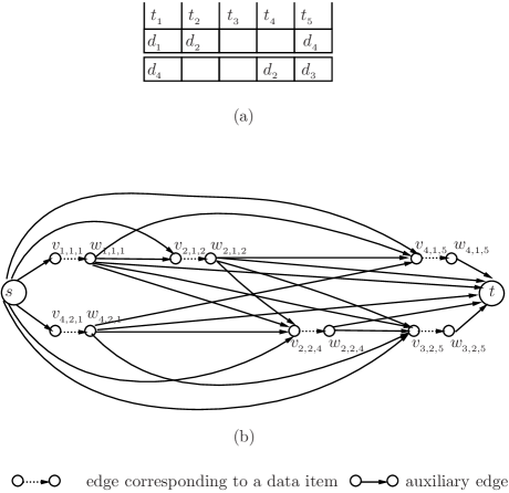
Figure 1: Construction of an auxiliary DAG for an instance of LWDR: (a) An instance of LWDR; (b) The corresponding auxiliary DAG.

II-B An Linear Programming Relaxation for $\delta$ALWDR

By Lemma 2, to compute an optimum solution to $\delta$ALWDR, we need only to compute $\delta$-disjoint maximum weight $st$-paths (with some additional restricts) in $G$. The following formula is an LP relaxation for $\delta$ALWDR (an LP relaxation for $\delta$ALNDR if $w(e)=1$ for all $e\in E$):

$$max \sum_{e\in E}w(e)x_{e}$$ (1)

$$s.t. \sum_{e\in E_{d_{i}}}x_{e}\leq 1\begin{array}[]{cc}&\forall E_{d_{i}}\subseteq E\end{array}$$ (7)

$$\sum_{e\in\delta^{+}(v)}x_{e}-\sum_{e\in\delta^{-}(v)}x_{e}=\left\{\begin{array}[]{cc}0&\mbox{ }\forall v\in V\setminus\{s,\,t\}\\ \delta&v=s\end{array}\right.$$

$$0\leq x_{e}\leq 1\mbox{ }\forall e\in E(G)$$

If Inequality (7) is removed, then the above formula is exactly an LP formula for the relaxation of $\delta$-disjoint $st$-paths in $G$. Because graph $G$ is acyclic, any integral optimum solution (i.e. a solution with all $x_{e}\in\{0,1\}$) to LP (1) contains no cycle. Thus, the solution is a set of (edge) disjoint paths with maximum weight, and hence an optimum solution to $\delta$ALWDR. Note that the condition that graph $G$ is acyclic is essential. Otherwise, a solution to LP (1) can contain both cycles and paths, and is not a solution to $\delta$ALWDR.

Further, since when $|E_{d_{i}}|=1$ holds for each $d_{i}$, the constraint matrix of LP (1) is known totally unimodular [18], we have the following property that indicates $\delta$ALWDR is polynomial solvable when each data item broadcast at most once:

Theorem 3.

When $|E_{d_{i}}|=1$ holds for each $d_{i}$, any basic optimum solution to LP (1) is integral, i.e., each edge $e$ is with $x_{e}=0$ or $x_{e}=1$.

Therefore, according to the theorem above, to solve an instance of $\delta$ALWDR in which each item appears at most once, we need only to compute a basic optimum solution to LP (1) with $\forall i$ $|E_{d_{i}}|=1$. Moreover, it is known that a basic optimum solution to LP (1) can be computed in polynomial time [14]. Hence, we have:

Corollary 4.

$\delta$ALWDR is polynomial solvable when each data item is broadcast at most once.

However, it is known the general case of $\delta$ALWDR is ${\cal NP}$-hard even when $\delta=1$. Worse still, it is hard to approximate $\delta$ALWDR within a factor better than $\frac{1}{2}$ via LP (1), as stated in the following observation:

Proposition 5.

The integrality gap of LP(1) is $\frac{1}{2}$, even for LNDR with only two channels and each data item is broadcast at most twice.

To show the integrality gap as above, we give an instance of LWDR as depicted in Figure 2, where there are only two channels, one antenna, and every item in the instance has the same weight and is broadcast at most twice. Then apparently, an optimal solution is to retrieve data items $\{d_{i}|i=1,\,3,\,\dots,\,2n-1\}$, for which the antenna only needs to keep listening to the upper channel. That is, the weight of the retrieved data items of an optimal solution is $n$. On the other hand, $\{x_{e}=\frac{1}{2}|e\in E_{d_{i}}\}$ is an optimal solution to LP (1) against the instance, resulting a weight of 2$n$.

Then following the definition of integrality gap, it is impossible to design an approximation algorithm with ratio better than 2 based on LP (1) (using LP-rounding, primal-dual method, etc). However, it is worth noting that the integrality gap of LP (1) is better than 2 if the occurrence assumption holds. In fact, that is why we propose the occurrence assumption.

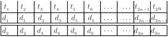
Figure 2: Integrality gap of LP (1).

III A Factor$-1-\frac{1}{e}$ Approximation Algorithm for $\delta$A$\gamma$LWDR

Instead of approximating $\delta$ALWDR directly, this section will first give an approximation algorithm with ratio $1-\frac{1}{e}$ for $\delta$A$\gamma$LWDR for $\delta=1$, and then show that it can be extended to general $\delta$. The key idea of the algorithm comes from the following simple observation that can be easily extended from a lemma in[16].

Proposition 6.

All possible $k$ retrieval sequences can be computed in $O(m^{kT})$ time for $\delta$ALWDR, where $T$ is the number of the time slots.

From the above proposition, a simple idea is first to solve each segment of $\delta$A$\gamma$LWDR individually (since a segment is an instance of $\delta$ALWDR with $\gamma$ time slots), and then to combine the computed subsolutions to a whole solution. However, the difficulty is how to guarantee that the subsolutions could compose a good solution. To overcome the difficulty, we first compute all possible paths for each segment of $\delta$A$\gamma$LWDR, then give a LP formula for $\delta$A$\gamma$LWDR based on the set of paths. Based on the formula, an approximation algorithm is developed by employing randomized rounding technique. The approximation achieves the same ratio of $1-\frac{1}{e}$ as in [16], but is simpler and can be easily extended to solve $\delta$A$\gamma$LWDR (and $\delta$ALWDR) for general $\delta$.

III-A The LP Formula for Relaxation of $\delta$A$\gamma$LWDR

Let $G$ be the auxiliary graph output by Algorithm 1. Let $t_{j_{0}}=t_{0},t_{j_{1}},\dots,t_{j{}_{l}}\dots$ be the vacant time slots in $\delta$A$\gamma$LWDR. Assume that $G_{i}$ is the part of $G$ between $t_{j_{i-1}}$ and $t_{j_{i}}$, i.e. it corresponds to the $i$th segment of $\delta$A$\gamma$LWDR. Let $\mathbb{P}=\{\mathbb{P}_{1},\dots,\mathbb{P}_{N}\}$, where $\mathbb{P}_{i}=\{P_{i,j}|j=1,\,\dots,\,h_{i}\,\mbox{and}\,|P_{i,j}\cap E_{d_{l}}|\leq 1\,\forall l\}$ is the set of all the possible paths of $G_{i}$ that correspond to retrieve sequences. Each $P_{i,j}$ is assigned with a weight $w(P_{i,j})=\sum_{e\in P_{i,j}}w(e)$. Formally, our LP relaxation for $\delta$A$\gamma$LWDR is as below:

$$max \sum_{i=1}^{N}\sum_{P_{i,j}\in\mathbb{P}_{i}}w(P_{i,j})\cdot x_{i,j}$$ (8)

$$s.t. \sum_{P_{i,j}\in\mathbb{P}_{i}}x_{i,j}=\delta\quad\forall\mathbb{P}_{i}\in\mathbb{P}$$ (11)

$$\sum_{i,j:\,P_{i,\,j}\cap E_{d_{l}}\neq\emptyset}x_{i,j}\leq 1\quad\forall E_{d_{l}}\subseteq E(G)$$

$$\quad\quad 0\leq x_{i,\,j}\leq 1\quad\forall P_{i,j}\in\mathbb{P}_{i}$$

In the above formula, $x_{i,j}=1$ indicates $P_{i,j}$ is selected, and $x_{i,j}=0$ otherwise. Inequality (11) is to guarantee that a feasible solution of LP (8) contains at most one edge of each $E_{d_{l}}$, i.e. at most one edge for item $d_{l}$. If $x_{i,j}\in\{0,1\}$ $1$, the above formula becomes an integral programming (IP) formula for $\delta$A$\gamma$LWDR.

III-B The Randomized Algorithm for $\delta$A$\gamma$LWDR

Let $\chi=(x_{1,1}^{*},\,\dots,x_{i,j}^{*},\dots)$ be an optimal solution to LP (8), and $w_{LP}$ be its weight. The key idea of our algorithm is to interpret the fractional value $x_{i,j}^{*}$ as the probability of selecting $P_{i,j}$ for $\mathbb{P}_{i}$. Then the algorithm is formally as in Algorithm 2.

Input: $G$, $\mathbb{P}=\{\mathbb{P}_{1},\dots,\mathbb{P}_{N}\}$, where $\mathbb{P}_{i}=\{P_{i,j}|j=1,\,\dots,\,h_{i}\}$ is a collection of paths of $G_{i}$, with a weight $w(P_{i,j})=\sum_{e\in P_{i,j}}w(e)$;

Output: $\mathbb{C}$, a solution to $\delta$A$\gamma$LWDR for $\delta=1$.

1. $\mathbb{C}:=\emptyset$;

2. Solve LP (8) against $\mathbb{P}$ for $\delta=1$ by Karmarkar’s algorithm [18], and obtain an optimal solution $\mathbf{x}=(x_{1,1}^{*},\,\dots,x_{i,j}^{*},\dots)$;

3. For $i=1$ to $N$ do

   1. Set $P_{i}:=P_{i,\,j}$ with probability $x_{i,j}^{*}$; /* $P_{i}$ is the element selected in $\mathbb{P}_{i}$. */

   2. $\mathbb{C}:=\mathbb{C}\cup\{P_{i}\}$;

4. Return $\mathbb{C}$.

Algorithm 2 A randomized algorithm for $\delta$A$\gamma$LWDR.

Lemma 7.

Algorithm 2 is a randomized $(1-(\frac{K-1}{K})^{K})$-approximation algorithm with a time complexity of $O(m^{3.5\gamma}\cdot(\frac{T}{\gamma})^{3.5}\cdot L)$ for $\delta$A$\gamma$LWDR for $\delta=1$, where $L$ is the maximum length of input and $K$ is the maximum occurrence times of $e$ in all $P_{i,j}$.

Proof:

The runtime of Algorithm 2 is easy to calculate: Step 2 of the algorithm takes $O\left(\left(\sum_{i=1}^{N}|\mathbb{P}{}_{i}|\right)^{3.5}L\right)$ time to run Karmarkar’s algorithm, where $|\mathbb{P}_{i}|=O\left(m^{\gamma}\right)$. Then because other steps take trivial time compared to Step 2, the total time is $O(\left(N\cdot m^{\gamma}\right)^{3.5}L)=O(m^{3.5\gamma}\cdot(\frac{T}{\gamma})^{3.5}\cdot L)$.

For the ratio, let $SOL$ and $w_{SOL}$ be the output of the algorithm and its weight respectively. To calculate the expected value of the output of the algorithm, it remains only to compute the probability that none of the edges of $E_{d_{l}}$ is in any $P_{i,j}\in SOL$. Below is the probability that $E_{d_{l}}\cap P_{i,j}=\emptyset$ for every $P_{i,j}\in SOL$:

$$\prod_{i}\left(1-\sum_{j:\,E_{d_{l}}\cap P_{i,,j}\neq\emptyset}x_{i,j}^{*}\right)\leq\prod_{i,j:\,E_{d_{l}}\cap P_{i,,j}\neq\emptyset}\left(1-x_{i,j}^{*}\right).$$

Then since $\sum_{i,j:\,E_{d_{l}}\cap P_{i,,j}\neq\emptyset}x_{i,j}^{*}$ is fixed, we assume that

$$f=\prod_{i,j:\,E_{d_{l}}\cap P_{i,,j}\neq\emptyset}(1-x_{i,j}^{*})-\lambda\cdot\sum_{i,j:\,E_{d_{l}}\cap P_{i,,j}\neq\emptyset}x_{i,j}^{*}$$

. It is easy to see $f$ attains maximum when

$$\frac{\partial f}{\partial x_{i,j}^{*}}=\lambda\mbox{ }\forall i,j:\,u_{k}\in P_{i,j}.$$

That is, when all elements of $\left\{x_{i,j}^{*}|E_{d_{l}}\cap P_{i,,j}\neq\emptyset\right\}$ are the same, $\prod_{i,j:\,E_{d_{l}}\cap P_{i,,j}\neq\emptyset}(1-x_{i,j}^{*})$ attains maximum $(1-\frac{1}{K})^{K}$, where $K$ is the number of the occurrence times of any edge of $E_{d_{l}}$ appearing in all $P_{i,j}$. So edges of $E_{d_{l}}$ have a probability of at most $(1-\frac{1}{K})^{K}$ to be all absent from every $P_{i,j}$. Now we have all the ingredients for computing $E(w_{SOL})$, the expectation of $w_{SOL}$:

$$E(w_{SOL}) = w_{LP}-(\mbox{expected weight of the elements absenting every }P_{i,j})\cdot w_{LP}$$

$$\geq (1-(1-\frac{1}{K})^{K})\cdot w_{LP}$$

Since $w_{LP}$ is the weight of an optimal solution to LP (8), $w_{LP}$ is not less than $w_{OPT}$, the weight of an optimal solution to $\delta$A$\gamma$LWDR. Therefore, $E(w_{SOL})\geq(1-(1-\frac{1}{K})^{K})\cdot w_{OPT}$. This completes the proof. ∎

By simple arithmetical calculation, it is easy to see the ratio will be $0.75$ when $K=2$, be $0.704$ when $K=3$, and be $0.684$ when $K=4$. Further, following the inequality as in Proposition 8 below, the ratio of our algorithm would be not less than $\lim_{K\rightarrow+\infty}1-(\frac{K-1}{K})^{K}=1-\frac{1}{e}$.

Proposition 8.

$f(K)=1-(\frac{K-1}{K})^{K}$ is a monotone increasing function for $K\geq 2$.

Proof:

The derivative of $f(K)$ is as in the following:

$$f(K)^{\prime}=((\frac{K-1}{K})^{K})^{\prime}=(e^{K(\ln(K-1)-\ln K)})^{\prime}=e^{K(\ln(K-1)-\ln K)}\cdotp(\frac{1}{k-1}+\ln\frac{K-1}{K}).$$

Because for $K=2$, we have both $\frac{1}{k-1}+\ln\frac{K-1}{K}>0$ and its derivative $(\frac{1}{k-1}+\ln\frac{K-1}{K})^{\prime}=\frac{1}{(K-1)^{2}}>0$, $f(K)^{\prime}>0$ holds for any $K\geq 2$. That is, for any $K\geq 2$, $f(K)$ is monotone increasing. ∎

The derandomization of Algorithm 2 to $\delta$A$\gamma$LWDR follows a similar line as the derandomization of Section 4 (although it is a little more complicated). So we omit it here.

III-C Extension to $\delta$A$\gamma$LWDR

In this subsection, Algorithm 2 is extended to solve $\delta$ALWDR for general $\delta$. To do this, two changes are needed for the algorithm: the first is to change the formula of LP (8), by setting the right part of the constraint of Equality (11) from 1 to $\delta$ accordingly; the second is to select $\delta$ disjoint paths to round up simultaneously for each $\mathbb{P}_{h}$, while Algorithm 2 round up only one path for each $\mathbb{P}_{h}$. More precisely, the second is to modify Step 3 of Algorithm 2 as below:

For each $\{P_{h,j_{1}},\dots,P_{h,j_{\delta}}\}\subseteq\mathbb{P}_{h}$ with $P_{h,j_{i}}\cap P_{h,j_{k}}=\emptyset$ for $j_{i}\neq j_{k}$ do

(a) Set $\mathbb{{\cal P}}_{h}:=\{P_{h,j_{1}},\dots,P_{h,j_{\delta}}\}$ with probability $\frac{\sum_{l=1}^{\delta}x_{i,j_{l}}^{*}}{\delta}$, where $\{P_{h,j_{1}},\dots,P_{h,j_{\delta}}\}$ is a set of $\delta$ disjoint paths in $\mathbb{P}_{h}$ and $\mathbb{{\cal P}}_{h}$ is the set of $\delta$ paths selected from $\mathbb{P}_{h}$.

(b) $\mathbb{C}:=\mathbb{C}\cup\mathbb{{\cal P}}_{h}$.

Lemma 9.

$\delta$A$\gamma$LWDR admits an approximation algorithm with ratio $1-\frac{1}{e}$ and runtime $O(m^{3.5\gamma}\cdot(\frac{T}{\gamma})^{3.5}\cdot L+\frac{T}{\gamma}m^{\delta\gamma})$.

Proof:

The ratio can be obtained following exactly the same line of Lemma 7.

For the time complexity, Step 2 takes $O(m^{3.5\gamma}\cdot(\frac{T}{\gamma})^{3.5}\cdot L)$ time to solve LP (8). Step 3 takes $\left(\begin{array}[]{c}m^{\gamma}\\ \delta\end{array}\right)=O(m^{\delta\gamma})$ time to select a ${\cal P}_{h}$ to round up, since it has to select $\delta$ paths among $m^{\gamma}$ paths which are all possible paths in $\mathbb{P}_{i}$. Therefore, the total runtime is $O(m^{3.5\gamma}\cdot(\frac{T}{\gamma})^{3.5}\cdot L+\frac{T}{\gamma}m^{\delta\gamma})$. This completes the proof. ∎

IV Approximation Algorithms for $\delta$A$\gamma$LWDR under Occurrence Assumption

The section will give an algorithm to approximate $\delta$A$\gamma$LWDR within a factor of $1-\frac{1}{e}$ for general $\delta$, under the occurrence assumption that every item is broadcast at most once in each segment. To do this, an approximation algorithm is first given for $\delta$A$\gamma$LWDR for $\delta=1$, with the key idea of collectively and randomly rounding fractional edges according to an optimum solution to LP (1). Later, the algorithm is derandomized using an interesting method based on conditional expectation.

For all the algorithms in this section, the key observation is that the high time complexity of Algorithm 2 mainly comes from the large size of $\mathbb{P}_{i}$, $m^{\gamma}$, where $m$ is the number of the channels and $\gamma$ the length of a segment. The basic idea of the algorithms is to compute the necessary paths only, instead of computing all possible paths. To do this, we release paths (or more precisely subflows) from the fractional flow of an optimum solution to LP (1). Those released paths compose the set of necessary paths for each $\mathbb{P}_{i}$. An integral solution to $\delta$A$\gamma$LWDR can then be obtained by rounding such fractional paths.

IV-A A Randomized Algorithm for $\delta$A$\gamma$LWDR under Occurrence Assumption

Our algorithm is mainly composed by the following steps: first to compute an optimum solution against LP (1) for the constructed graph $G$, output by Algorithm 1 for an given $\delta$A$\gamma$LWDR instance; then for each $\gamma$-separated segment, the algorithm releases a set of subflows with fractional value from the computed solution; later, the value of each subflow is randomly rounded to 1 with probability proportional to the original value. Eventually, the combination of the rounded subflows of each $\gamma$-separated segment will collectively compose an integral solution to $\delta$A$\gamma$LWDR. The full layout of the algorithm is as in Algorithm 3.

Input: Auxiliary graph $G$ corresponding to an instance of $\delta$A$\gamma$LWDR with occurrence assumption and $\delta=1$, in which $G_{i}$ is corresponding for the $i$th segment of $\delta$A$\gamma$LWDR;

Output: A solution to $\delta$A$\gamma$LWDR.

1. Solve LP (1) against $G$ by Karmarkar’s algorithm [18], and obtain an optimal solution $\mathbf{x}=(x_{1,1,1}^{*},\,\dots,x_{i,j,k}^{*},\dots)$;

2. For $h=1$ to $N$ do

   1. For the flow corresponding to $\mathbf{x}$, divide the part in $G_{h}$ into a set of subflows, say $\mathbb{F}_{h}=\{f_{h,1},\,\dots,\,f_{h,\,j_{h}}\}$ where $f_{h,\,j}$ is with value $y_{h,\,j}$, $j\in\{1,\,\dots,\,j_{h}\}$ by using Algorithm 4 (given later);

   2. Round the value of $f{}_{h,\,j}$ to 1 with probability $y_{h,\,j}$;

3. Return the set of the subflows with value 1 as a solution to $\delta$A$\gamma$LWDR.

Algorithm 3 A collective randomized rounding algorithm for $\delta$A$\gamma$LWDR.

Lemma 10.

Algorithm 3 outputs a solution for $\delta$A$\gamma$LWDR within runtime $O(|E(G)|{}^{3.5}L)$, where $L$ is the maximum length of the input.

Proof:

Step 1 of the algorithm runs Karmarkar’s algorithm and takes $O(|E(G)|{}^{3.5}L)$ time to solve LP(8) wrt the auxiliary graph $G$, since the number of the constraints of LP (8) is $O(|E(G)|+|V(G)|)=O(|E(G)|)$. According to Lemma 11 (which is given later), Step 2 takes $O(|E(G_{h})|^{2})$ time to compute each $\mathbb{F}_{h}$, and the rounding time for each $\mathbb{F}_{h}$ is $O(|\mathbb{F}_{h}|)=O(|E(G_{h})|^{2})$. So the total time of Step 2 is $O(N\cdot|E(G_{h})|^{2})$. Therefore, the total time complexity of Algorithm 3 is $O(|E(G)|{}^{3.5}L)$. ∎

Let $m$ be the number of channels and $T$ be the number of time slots. Recall that $|V(G)|$ equals to the number of all the occurrences of the data items $O(mT)$, and $|E(G)|=O(|V(G)|^{2})$ according to the construction of $G$ as Algorithm 1. However, as will be shown in Section V, $|E(G)|$ can be decreased to $O(m\cdot|V(G)|)=O(m^{2}T)$. So the runtime of Algorithm 3 is actually $O(m^{7}T^{3.5}L)$.

Lemma 11.

Algorithm 3 is a randomized $(1-(\frac{K-1}{K})^{K})$-approximation algorithm for $\delta$A$\gamma$LWDR, where $K$ is the maximum occurrence times of $d_{i}$ in the subflows in the time interval.

Proof:

Let $SOL$ and $OPT$ be the output of the algorithm and the optimum solution of $\delta$A$\gamma$LWDR, respectively. We shall show $E(w(SOL))\geq w(OPT)\cdot(1-(\frac{K-1}{K})^{K})$, where $E(w(SOL))$ is the expectation of $w(SOL)$. Let $w_{LP}$ be the weight of an optimum solution to LP (1) against $G$. Since $w(OPT)\leq w_{LP}$, it remains only to show $E(w(SOL))\geq w_{LP}\cdot(1-(\frac{K-1}{K})^{K})$. Thus, we will calculate how much weight is expected to lose during the rounding procession. For item $d_{i}$, assume that

$$\sum_{j,k,h,l:\,e_{i,j,k}\in f_{h,l}}y_{h,l} = \alpha,\,\,\,\,\,\,0\leq\alpha\leq 1,$$

where $y_{h,l}$ is the value of flow $f_{h,l}$ which contains $e_{i,j,k}$. Then the probability that the algorithm does not pick $d_{i}$ is:

$$(1-\alpha)+\alpha\cdot\prod_{j,k,h,l:\,e_{i,j,k}\in f_{h,l}}(\alpha-y_{h,l}).$$

Then since $\sum_{j,k,h,l:\,e_{i,j,k}\in f_{h,l}}y_{h,l}=\alpha$ is fixed, we assume that $g_{i}=\prod_{j,k,h,l:\,e_{i,j,k}\in f_{h,l}}(\alpha-y_{h,l})-\lambda\cdot\sum_{j,k,h,l:\,e_{i,j,k}\in f_{h,l}}y_{h,l}$. Similar to the proof of Lemma 7, it is easy to see $g_{i}$ attains maximum when

$$\frac{\partial g_{i}}{\partial y_{h,l}}=0\mbox{ }\forall j,k,h,l:\,e_{i,j,k}\in f_{h,l}.$$

That is, $g_{i}$ attains maximum when every $y_{h,l}:\,f_{h,l}\supseteq\{e_{i,j,k}\}$ is with the same value. Then the probability that the algorithm does not pick any edge corresponding to $d_{i}$ is at most:

$$(1-\alpha)+\alpha\cdot(1-\frac{1}{K})^{K},$$

where $K$ is the number of the occurrences of $e_{i,j,k}$, $\forall j,\,k$, in all subflows, i.e. $f_{h,\,l}$, $\forall h,\,l$. So the expectation of item $d_{i}$ being picked is $\alpha(1-(1-\frac{1}{K})^{K})$. Therefore the expectation of $w(SOL)$ is:

$$E(w(SOL)) = w_{LP}\left(\frac{\mbox{the probability of the edges responding to $d_{i}$appearing in any }f_{l}}{\alpha}\right)$$

$$\geq (1-(1-\frac{1}{K})^{K})\cdot w_{LP}$$

This completes the proof. ∎

It remains to give the division of the subflows for Algorithm 3. Let $\mathbf{x}=(x_{1,1,1}^{*},\,\dots,x_{i,j,k}^{*},\,\dots)$ be an optimal solution to LP (8). W.l.o.g., assume that we are processing the edges of $G_{h}$, and $E_{h}=\{e|0<x_{e}\leq 1\}$, i.e. $E_{h}$ is the set of edges with $0<x_{e}\leq 1$ in $G_{h}$. The key idea of the computation is to repeatedly select an edge $e$ with minimum $x_{e}$, and then construct in $E_{h}$ a flow (which is also a single path) of value $x_{e}$ going through $e$, until every edge $e$ in $E_{h}$ is with $x_{e}=0$. The detailed algorithm is shown in Algorithm 4.

Input: $G_{h}$, $E_{h}$ and $\mathbf{x}=(x_{1,1,1}^{*},\,\dots,x_{i,j,k}^{*},\dots)$, an optimum solution to LP (1);

Output: $\mathbb{F}_{h}$.

1. Set $\mathbb{F}_{h}:=\emptyset$, $i:=1$;

2. Set $e^{*}:=nil$, $x{}_{e^{*}}:=0$, $f_{h,i}:=\emptyset$;

3. For each $e\in E_{h}$ do

   1. If $x_{e}<x_{e^{*}}$ then

      $e^{*}:=e$;

   /*Find an edge $e^{*}\in E_{h}$ with $x_{e^{*}}\leq x_{e}$ for any $e\in E_{h}$. */

4. $f_{h,i}:=f_{h,i}\cup\{e^{*}\}$;

5. Set $e_{pre}:=e_{suc}:=e^{*}$;

6. While $e_{pre}$ has preceding edges do

   1. Select one of the preceding edges, say $e$;

   2. Set $x_{e}:=x_{e}-x_{e^{*}}$, $e_{pre}:=e$, and $f_{h,i}:=f_{h,i}\cup\{e^{*}\}$;

   EndWhile

   /*Add the part of $f_{h,i}$ before $e^{*}$ to $f_{h,i}$.*/

7. While $e_{suc}$ has successor edges do

   1. Select one of the successor edges, say $e$;

   2. Set $x_{e}:=x_{e}-x_{e^{*}}$, $e_{suc}:=e$, and $f_{h,i}:=f_{h,i}\cup\{e_{suc}\}$;

   EndWhile

   /*Add the part of $f_{h,i}$ after $e^{*}$ to $f_{h,i}$.*/

8. Set $x_{e^{*}}:=0$ and $\mathbb{F}_{h}:=\mathbb{F}_{h}\cup f_{h,i}$; /*Add $f_{h,i}$ to $\mathbb{F}_{h}$.*/

9. For each $e\in E_{h}$ do

      If $x_{e}=0$ then $E_{h}:=E_{h}\setminus\{e\}$;

10. If $E_{h}\neq\emptyset$ then

       Set $i:=i+1$ and go to Step 2;

    Else return $\mathbb{F}_{h}$.

Algorithm 4 Computation of $\mathbb{F}_{h}$.

Lemma 12.

Algorithm 4 runs in $O(|E(G_{h})|^{2})$ time, and correctly computes a set of flows $\mathbb{F}_{h}=\{f_{h,i}\}$ for $G_{h}$, such that $|\mathbb{F}_{h}|\leq|E(G_{h})|$ and $x_{e}=\sum_{h,i:\,e\in f_{h,i}}y_{h,i}$ holds for each $e\in G_{h}$.

Proof:

Algorithm 4 iterates Step 2-10 at most $|E_{h}|$ times, since each iteration removes at least one edge from $E_{h}$. In each iteration, Step 6 and 7 need to verify all edges of $E_{h}$ in the worst case, which is at most $O(E_{h})$. So Algorithm 4 runs in $O(|E(G_{h})|^{2})$ time.

For $|\mathbb{F}_{h}|$, according to Algorithm 4, the size of $E_{h}$ decreases at least one when a new flow is added to $\mathbb{F}_{h}$, since at least an edge $e^{*}$ with its $x_{e^{*}}$ set to 0 is removed from $E_{h}$. So $|\mathbb{F}_{h}|\leq|E_{h}|\leq|E(G_{h})|$. For the latter part, $x_{e}=\sum_{h,i:\,e\in f_{h,i}}y_{h,i}$ clearly holds since Algorithm 4 decreases $y_{h,i}$ from $x_{e}$ if and only if $e\in f_{h,i}$. ∎

Similar to the extension of Algorithm 2 to $\delta$A$\gamma$LWDR, and the analysis of Lemma 9, it is easy to extend Algorithm 3 to $\delta$A$\gamma$LWDR for general $\delta$. Hence, the extension is omitted.

IV-B Derandomization

The main idea of our derandomization is inspired by the derandomization technique using conditional expectations as implicitly given in [4] and formally given in the book [20]. That is, to pick $f_{i,j}$ for $\mathbb{F}_{i}$ in a greedy and sequential way: the flow for $\mathbb{F}_{1}$ is first to select, then $\mathbb{F}_{2}$, $\mathbb{F}_{3}$, $\dots$, and so on. Assume that the selection of the flow for $\mathbb{F}_{1},\dots,\mathbb{F}_{h}$ is complete, and the algorithm is currently selecting flow for $\mathbb{F}_{h+1}$ against $G^{h+1}=G\setminus\{G_{i}|1\leq i\leq h\}\setminus\{e|e\in f_{i,j_{i}^{*}},\,1\leq i\leq h\}$, where $f_{i,j_{i}^{*}}$ is the flow already selected (i.e., $y_{i,j_{i}^{*}}$ is rounded to 1) for $\mathbb{F}_{i}$, and $G^{h+1}$ contains only the edges corresponding to data items to be covered in future. Our algorithm selects for $\mathbb{F}_{h+1}$ for the flow $f_{h+1,\,j_{h+1}^{*}}$ with $w(f_{i,h+1})+w(\mathbf{x}(G^{h+1}))$ maximized. The detailed algorithm is shown in Algorithm 5. Why the algorithm removes the edges of $\{e|e\in f_{i,j_{i}^{*}},\,1\leq i\leq h\}$ from $G^{h+1}$ is that, if the edge corresponding to item $d_{l}$ is already in $\mathbb{F}_{i}:\,i\leq h$, the weight of the retrieve sequence will not increase by covering any edge corresponding to the same item $d_{l}$ for later processing.

Input: $\mathbb{F}=\{\mathbb{F}_{1},\dots,\mathbb{F}_{N}\}$, where $\mathbb{F}_{i}=\{f_{i,\,j}\}$ is a collection of flows for the $i$th segment of $\delta$A$\gamma$LWDR;

Output: $\mathbb{C}$, a solution to $\delta$A$\gamma$LWDR.

1. $\mathbb{C}:=\emptyset$;

2. Solve LP (1) by Karmarkar’s algorithm [18], and obtain an optimum solution $\mathbf{x}$;

3. For $i=1$ to $N$ do

   1. For each $f_{i,j}\in\mathbb{F}_{i}$ do

      Set $z_{i,j}:=w(f_{i,j})+w(\mathbf{x}(G^{i}\setminus f_{i,j}))$;

      /* $z_{i,j}$ is the weight of $f_{i,j}$ plus the expected weight sum of edge $e\in G^{i}\setminus f_{i,j}$ selected at probability $x_{e}$. */

   2. Select $j_{i}^{*}$, such that $z_{i,j_{i}^{*}}\geq z_{i,j}$ for every $f_{i,j}\in\mathbb{F}_{i}$;

   3. $\mathbb{C}:=\mathbb{C}\cup\{f_{i,j_{i}^{*}}\}$

4. Return $\mathbb{C}$.

Algorithm 5 Derandomization of Algorithm 3.

Lemma 13.

The ratio of Algorithm 5 is $1-\frac{1}{e}$.

Proof:

Let $E(w(\mathbf{x}(G^{h})))$ denote the expectation weight sum of edges $e\in G^{h}$ picked at probability $x_{e}$, i.e.

$$E\left(w\left(\mathbf{x}\left(G^{h}\right)\right)\right)=\sum_{i=1}^{j_{h}}y_{i,j_{i}}\cdot\left(w\left(f_{i,j_{i}}\right)+E\left(w\left(\mathbf{x}\left(G^{h}\setminus f_{i,j_{i}}\right)\right)\right)\right)$$ (13)

Then $E(w(\mathbf{x}(G^{1})))$ is equal to $E(w(SOL))$, the expectation of the weight of the output of Algorithm 3. So we need only to show $\sum_{i=1}^{N}w(f_{i,j_{i}^{*}})\geq E(w(\mathbf{x}(G^{1})))$, provided that $E(w(SOL))\geq(1-\frac{1}{e})w(OPT)$ holds according to Lemma 11.

First, for the last iteration, the algorithm picks $f_{N,\,j_{N}^{*}}$ with maximum $z_{N,j}:=w(f_{N,j})$ among all $j$s in $G^{N}$, so the following inequality obviously holds:

$$w(f_{N,j_{N}^{*}})\geq E(w(\mathbf{x}(G^{N}))).$$ (14)

Consider that we are selecting for $h$, then since $j_{h}^{*}$ is chosen to attain maximum $z_{h,j_{h}^{*}}$, we have:

$$\begin{array}[]{ccc}w\left(f_{h,j_{h}^{*}}\right)+E\left(w\left(\mathbf{x}\left(G^{h+1}\right)\right)\right)&\geq&\sum_{i=1}^{j_{h}}y_{i,j_{i}}\cdot\left(w\left(f_{i,j_{i}}\right)+E\left(w\left(\mathbf{x}\left(G^{h}\setminus f_{i,j_{i}}\right)\right)\right)\right)\end{array}$$ (15)

Then, combining Inequality (13) and (15) yields

$$w\left(f_{h,j_{h}^{*}}\right)+E\left(w\left(\mathbf{x}\left(G^{h+1}\right)\right)\right)\geq E\left(w\left(\mathbf{x}\left(G^{h}\right)\right)\right).$$ (16)

Summing up Inequality (16) for every $1\leq h\leq N-1$, and combining with Inequality (14), we have:

$$\sum_{h=1}^{N}w\left(f_{h,j_{h}^{*}}\right)+\sum_{h=1}^{N-1}E\left(w\left(\mathbf{x}\left(G^{h+1}\right)\right)\right)\geq\sum_{h=1}^{N}E\left(w\left(\mathbf{x}\left(G^{h}\right)\right)\right).$$

That is, $\sum_{i=1}^{N}w(f_{i,j_{i}^{*}})\geq E(w(\mathbf{x}(G^{1})))$. This completes the proof. ∎

V An Improved Approximation Algorithm for General $\delta$A$\gamma$LWDR

In this section, we shall show that Algorithm 3 can be extended to approximate general $\delta$A$\gamma$LWDR within the same factor of $1-\frac{1}{e}$, without the occurrence assumption. The key observation is that Algorithm 3 cannot produce a good approximation ratio for $\delta$A$\gamma$LWDR since a fractional flow can contain two edges corresponding to an identical data item. So the idea of the extension is to construct an improved auxiliary graph in which different edges of an identical flow is corresponding to distinct data items. Then, the algorithm is to employ the collectively flow rounding method based on LP (17) given in this section against the improved auxiliary graph, and obtain an approximation solution with the same ratio $1-\frac{1}{e}$.

V-A A Refined Construction and a Dual LP Formula

Before giving the auxiliary graph where our algorithm can work correctly, we would like first to give a refined construction of $G$, which significantly decreases the number of edges of $G$, from $O(|V(G)|^{2})$ to $O(m\cdot|V(G)|)$, where $m$ is the number of the channels. The key observation of the refined construction is that for a valid retrieve sequence of LWDR, the constructed graph need only to contain an $st$-path with all the edges, but not necessarily exactly the same edges corresponding to the data items in the retrieve sequence. Hence, we need only to construct a DAG satisfying Lemma 14. The key idea of the construction is to connect the head of an edge to only one edge in every channel.

However, as analyzed later, LP (1) is not suitable for $\delta$A$\gamma$LWDR with respect to the construction. Besides the main part of $G$, it requires an additional virtual part to collaborate a new LP relaxation. The full layout of the construction is in Algorithm 6.

Input: An instance of $\delta$A$\gamma$LWDR;

Output: $G$.

1. Set $G:=\emptyset$, $G_{v}:=\emptyset$, $G_{r}:=\emptyset$; /*Initialization. $G_{r}$ is for the main part that corresponding to $\delta$A$\gamma$LWDR; $G_{v}$ the additional virtual part for a new LP relaxation.*/

2. For every item $d_{i}$:

   Add an edge set $E_{d_{i}}=\{e_{i,j,k}=(v_{i,j,k},\,w_{i,j,k})|d_{i}\mbox{ appears in channel $j$in the }k\mbox{th time slot}\}$ to $G_{r}$, where $w(e_{i,j,k})=w_{i}$;

3. Add two vertices $s$ and $p$ with weight-0 edges to $G_{r}$ as below:

   1. Edge $(s,\,v_{i,j,k})$ with minimum $k$ for every $j$;

   2. Edge $(w_{i,j,k},\,p)$ with maximum $k$ for every $j$;;

4. For $j=1$ to $m$ do

   For $k=1$ to $T$ do  /* Add edges for the relationship between the items. */

   If edge $(v{}_{i,j,k},\,w_{i,j,k})$ exists then

   Add weight-0 edge $(w{}_{i,j,k},\,v_{i^{\prime},j,k^{\prime}})$ to $G_{r}$ with minimum $k^{\prime}>k$;

   Add weight-0 edge $(w_{i,j,k},\,v_{i^{\prime},j^{\prime},k^{\prime}})$ to $G_{r}$ with minimum $k^{\prime}>k+1$ for every $j^{\prime}\neq j$;

   EndIf

   /*For each item add an edge from $v{}_{i,j,k}$ to the tail of the edge corresponding to the nearest item that could be retrieved conflict-freely afterward.*/

5. For every item $d_{i}$ do

   Add edges $e_{i}=(u_{T+i},v_{T+i})$ and $e^{\prime}_{i}=(u^{\prime}_{T+i},v^{\prime}_{T+i})$, as well as the edges $e_{i}=(u_{T+i},v^{\prime}_{T+i})$ and $e^{\prime}_{i}=(u^{\prime}_{T+i},v_{T+i})$, to $G_{v}$ where $c(e_{i})=1$ and $w(e_{i})=w(d_{i})$, other edges are all with cost 0.

   /* The construction of $G_{v}$. Note that $v_{T+i}=u_{T+i+1}$, $v^{\prime}_{T+i}=u^{\prime}_{T+i+1}$, and $u_{T+n}=u^{\prime}_{T+n}=t$.*/

6. Add edges $e(p,u_{T+1})$ and $e(p,u^{\prime}_{T+1})$ to $G_{v}$;

   /* Add the connection between $G_{r}$ and $G_{v}$. */

7. Return $G:=G_{r}\cup G_{v}$.

Algorithm 6 Construction of Auxiliary Graph for $\delta$A$\gamma$LWDR.

Lemma 14.

$S$ is a valid retrieve sequence for $\delta$A$\gamma$LWDR if and only if in the constructed graph of Algorithm 6 there exist $\delta$ disjoint $st$-paths whose corresponding retrieve sequences contain every item of $S$.

Proof:

We shall only show the lemma holds for the case $\delta=1$, since the case for general $\delta$ is similar.

For the “only if” direction, let $S=o_{i_{1},j_{1},k_{1}},o_{i_{2},j_{2},k_{2}},\dots o_{i_{l},j_{l},k_{l}},o_{i_{l+1},j_{l+1},k_{l+1}},\dots$, $k_{l+1}>k_{l}$ for any $l$, be a retrieve sequence for an instance LWDR, where $o_{i_{l},j_{l},k_{l}}$ is data item $d_{i_{l}}$ retrieved in channel $j_{l}$ and time slot $k_{l}$. If $o_{i_{l+1},j_{l+1},k_{l+1}}$ can be retrieved after $o_{i_{l},j_{l},k_{l}}$, then the two data items must be conflict-free. That is, $o_{i_{l+1},j_{l+1},k_{l+1}}$ and $o_{i_{l},j_{l},k_{l}}$ are either (1) in the same channel, i.e. $j_{l_{1+1}}=j_{l}$; or (2) in different channels and $k_{l+1}-k_{l}\geq 2$. According to the construction of $G$, there will be an edge leaving $w_{i_{l},j_{l},k_{l}}$, the head of the edge corresponding to item $o_{i_{l},j_{l},k_{l}}$, and entering $v{}_{i_{l+1},j_{l+1},k^{\prime}}$, the tail of the edge corresponding to a conflict-free data item $o_{i_{l+1},j_{l+1},k^{\prime}}$ for the minimum $k^{\prime}>k_{l}$. Then according to the construction again, there exists a path from $o_{i_{l+1},j_{l+1},k^{\prime}}$ to $o_{i_{l+1},j_{l+1},k_{l+1}}$. That is, every $o_{i_{l+1},j_{l+1},k_{l+1}}$ is reachable from $v_{i_{l},j_{l},k_{l}}$. Therefore, $P=s,v_{i_{1},j_{1},k_{1}},w_{i_{1},j_{1},k_{1}},v_{i_{2},j_{2},k_{2}},w{}_{i_{2},j_{2},k_{2}},\dots,t$ is an $st$ path in $G$.

For the “if” direction, assume that there exists a path $P=s,v_{i_{1},j_{1},k_{1}},w_{i_{1},j_{1},k_{1}},v_{i_{2},j_{2},k_{2}},w_{i_{2},j_{2},k_{2}},\dots,$ $v_{i_{l},j_{l},k_{l}},w_{i_{l},j_{l},k_{l}},v_{i_{l+1},j_{l+1},k_{l+1}},w_{i_{l+1},j_{l+1},k_{l+1}},\dots,t$, $k_{l+1}>k_{l}$, in $G$. According to the construction, for any edge $(w_{i_{l},j_{l},k_{l}},v{}_{i_{l+1},j_{l+1},k_{l+1}})$, $k_{l+1}-k_{l}>1$ holds or $j_{l}=j_{l+1}$ and $k_{l+1}>k_{l}$ both hold. That is, the items retrieved in time slot $k_{l}$ and $k_{l+1}$, say $o_{i_{l},j_{l},k_{l}}$ and $o_{i_{l+1},j_{l+1},k_{l+1}}$ can be retrieved conflict-freely. So $o_{i_{1},j_{1},k_{1}},o_{i_{2},j_{2},k_{2}},\dots$ is a valid retrieve sequence. These completes the proof. ∎

It is easy to see that the DAG $G$ resulting from Algorithm 6 has a much smaller size compared to the previous construction as in Algorithm 1, as stated below:

Lemma 15.

In the constructed graph $G$, there exist at most $O(m\cdot T)$ vertices, and at most $O(m^{2}T)$ edges.

Proof:

Clearly, we have $|V(G)|=O(m\cdot T)$. That is because we add an edge for each occurrence of the data items in the construction, and the number of the occurrences is at most $O(m\cdot T)$. Then since there exist at most $m$ edges leaving a vertex, $E(G)\leq m\cdot|V(G)|=O(m^{2}T)$. ∎

We now argue that LP (1) is no longer a relaxation for $\delta$A$\gamma$LWDR with respect to the above refined construction. Because for a solution of $\delta$A$\gamma$LWDR, there might exist no $st$-path with exactly the edges corresponding to the retrieved sequence, i.e. because a path in $G$ might contain two edges that corresponding to an identical data item (See figure 3 for an example: The path, corresponding to the retrieve sequence containing $d_{1},d_{2},d_{3}$, is forced to go through both edges $(v_{2,1,2},w_{2,1,2})$ and $(v_{2,2,4},w_{2,2,4})$, which are corresponding to the an identical item). But according to Inequality (7), $\sum_{e\in E_{d_{i}}}x_{e}\leq 1$ should hold. Therefore, it remains to give a new LP formula for $\delta$A$\gamma$LWDR with respect to $G$ resulted from the refined construction. To do so, we first add a virtual part to $G$, and then give an LP formula, which allows a path in $G$ to contain multiple edges corresponding to an identical item. Then the LP formula is as below:

$$min \sum_{i=N+1}^{N+n}c(e_{i})\cdot w(e_{i})\cdotp x_{e_{i}}$$ (17)

$$s.t. \sum_{e\in\delta^{+}(v)}x_{e}-\sum_{e\in\delta^{-}(v)}x_{e}=\left\{\begin{array}[]{cc}0&\mbox{ }\quad\forall v\in V\setminus\{s,\,t\}\\ \delta&v=s\end{array}\right.$$ (22)

$$\sum_{j,k}x_{e_{i,j,k}}\geq 1\,\quad\quad\quad\quad\quad\quad\quad\quad\mbox{ }1\leq i\leq n$$

$$0\leq x_{e}\leq 1\,\quad\quad\quad\quad\quad\quad\quad\quad\quad\mbox{ }\forall e\in G$$

where $x_{e}=1$ iff $e$ is selected and $x_{e}=0$ otherwise. If $x_{e}\in\{0,\,1\}$, then from Lemma 14, the above formula becomes an integral programming (IP) formula for $\delta$A$\gamma$LWDR. The intuitive explanation of the above LP is as below: Let $W=\sum_{i=1}^{n}w_{i}$, let $c_{IP}$ be the minimum of the objective function of the IP corresponding to LP (8), and let $w_{OPT}$ be the weight of an optimal solution to the corresponding $\delta$A$\gamma$LWDR instance. Then, we have

$$W=c_{IP}+w_{OPT}.$$ (23)

Because $W$ is fixed, it is identical either to maximize $w_{OPT}$ or to minimize $c_{IP}$.

Then based on the new LP formula, Algorithm 3 can be immediately adopted to solve $\delta$A$\gamma$LWDR. Following the same line of Lemma 11 and 10, and then Lemma 15 on the sized of $G$, we have the following Theorem:

Theorem 16.

Under the occurrence assumption, $\delta$A$\gamma$LWDR admits an algorithm with ratio $1-\frac{1}{e}$ and a time complexity $O(m^{7}T^{3.5}L)$.

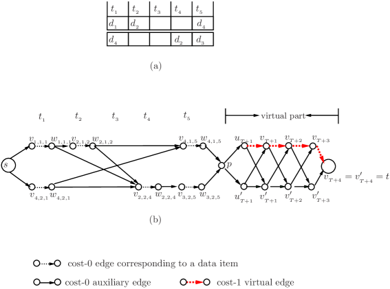
Figure 3: A refined construction of DAG: (a) An instance of LWDR; (b) The refined corresponding graph.

V-B Construction of the Improved Auxiliary Graph

This subsection will further improve the auxiliary graph output by Algorithm 6, such that in the improved auxiliary graph any path in a segment will not go through two edges corresponding to an identical data item. Thus, the improved auxiliary graph can be considered as a graph satisfying the occurrence assumption, and hence Algorithm 3 can be employed to solve the $\delta$A$\gamma$LWDR problem accordingly. The key idea of the improved construction is to find and eliminate every pair of edges which correspond to an identical data item and appear in a common path within a segment. The detailed construction of the improved auxiliary graph is in Algorithm 7, where w.l.o.g. we assume the $\delta$A$\gamma$LWDR instance has only one segment, since the case for multiple segments is similar. An example of execution of the algorithm is depicted in Figure 4.

Input: A refined auxiliary graph $G$ (for $\delta$A$\gamma$LWDR with one segment) output by Algorithm 6;

Output: A graph $G^{\prime}$, in which no flow exists containing two edges corresponding to an identical data item.

1. $G^{\prime}:=G$;

2. For $h=1$ to $T$ do

   1. For each edge $e=(v,\,w)\in G[t_{h+1},\,p]$ do /*$G[t_{h+1},\,p]$ is the subgraph of $G$ from time slot $t_{h+1}$ to $p$.*/

      Add a corresponding edge duplicating $e$, say $e^{(k)}=(v^{(k)},\,w^{(k)})$, to $G^{{}^{\prime}}$, assuming it is the $k$th time duplicating $e$;

      /*Duplicate $G[t_{h+1},\,p]$ by duplicating every edge therein. */

   2. For $j=1$ to $m$ do

      while there exist both edge $(v_{i,j,h},w_{i,j,h})$ and edge $(v_{i,j^{\prime},h^{\prime}},w{}_{i,j^{\prime},h^{\prime}})$ with $h^{\prime}>h$, such that $v_{i,j^{\prime},h^{\prime}}$ is reachable from $w_{i,j,h}$ do

      /*There exist a path containing 2 edges both corresponding to item $d_{i}$.*/

      (i) Replace each edge ended at $v_{i,j,h}$, say $e(v,v_{i,j,h})$, with $e(v,w{}_{i,j,h})$ in $G^{\prime}$;

      (ii) Replace each edge ended at $v_{i,j^{\prime},h^{\prime}}^{(k)}$, say $e(v,v_{i,j^{\prime},h^{\prime}}^{(k)})$, with $e(v,w{}_{i,j^{\prime},h^{\prime}}^{(k)})$ in $G^{\prime}$;

   Endfor

3. Return $G^{\prime}$.

Algorithm 7 The construction of an improved auxiliary graph.

Lemma 17.

In runtime $O(2^{\gamma}|E(G)|)$, Algorithm 7 outputs a graph $G^{\prime}$ with at most $O(2^{\gamma}|E(G)|)$ edges, where $\gamma$ is the maximum length of a segment of $\delta$A$\gamma$LWDR. $G^{\prime}$ has a size, i.e. $\max\{E(G^{\prime}),V(G^{\prime})\}$, not larger than $2^{\gamma}\cdot|E(G)|$, and every path therein contains at most one edge of $E_{d_{i}}$ for each item $d_{i}$ within a segment.

Proof:

For the time complexity, Step 2 of Algorithm 7 repeats at most $O(\gamma)$ times, each of which at most doubles the size of $G^{\prime}$. Since $G^{\prime}$ is initially $G$, $|E(G^{\prime})|\leq 2^{h-1}\cdot|E(G)|$ holds at the beginning of the $h$th iteration. In this iteration, it takes $O(E(G^{\prime}))$ time to duplicate the edges (in Step 2(a)) and takes $O(E(G^{\prime}))$ time to check for $(v_{i,j,k},w_{i,j,k})$ for every $j$ that whether there exists a path containing 2 edges both corresponding to an identical item (in Step 2(c)). So the total runtime of the algorithm is $\sum_{h=1}^{\gamma}O(2^{h-1}\cdot|E(G)|)=O(2^{\gamma}\cdot|E(G)|)$. In addition, we also have $E(G^{\prime})=O(2^{\gamma}\cdot|E(G)|)$.

According to Algorithm 7, the $h$th iteration guarantees that no path can contain both edge $(v_{i,j,h},w{}_{i,j,h})$ and another edge corresponding to $d_{i}$. Therefore, when Algorithm 7 terminates, all paths containing 2 edges corresponding to an identical item are eliminated. This completes the proof. ∎

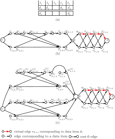
Figure 4: An construction of the improved DAG.

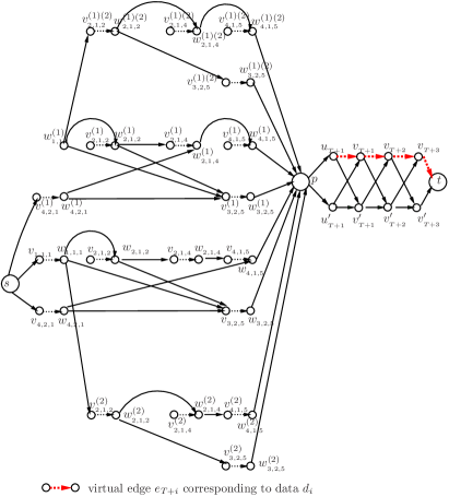
Figure 5: An construction of the improved DAG (continued)

The correctness of Algorithm 7 can be immediately obtained from the following lemma:

Lemma 18.

There exists $\delta$-disjoint $st$-path $P_{1},\,\dots,\,P_{\delta}$ in $G$ if and only if there exists in $G^{\prime}$ $\delta$ disjoint $st$-paths $Q_{1},\dots,Q_{\delta}$, such that their corresponding retrieve sequences contain identical data items.

Proof:

Let $e_{i,j,k}$ and $e_{i^{\prime},j^{\prime},k^{\prime}}$ be two edges in $G$ output by Algorithm 6, where $e_{i,j,k}$ means that data item $d_{i}$ appears in channel $j$ at time slot $k$. According to the construction of $G^{\prime}$ as in Algorithm 7, if $e_{i,j,k}$ and $e_{i^{\prime},j^{\prime},k^{\prime}}$ connected in $G$, then any duplication of $e_{i,j,k}$ and that of $e_{i^{\prime},j^{\prime},k^{\prime}}$ are connected in $G^{\prime}$ when $i\neq i^{\prime}$. Let $P$ containing edges $\{e_{i_{1},j_{1},k_{1}},\,\dots,\,e_{i_{h},j_{h},k_{h}}\}$, $k_{l}<k_{l+1}$, be a path in $G$, where e $k_{l}$ is the minimum time slot where $d_{i_{l}}$’s corresponding edges appear on the path $P$. Then there must exist a path $Q$ containing $\{e_{i_{1},j_{1},k_{1}}^{(*)},\,\dots,\,e_{i_{h},j_{h},k_{h}}^{(*)}\}$ in $G^{\prime}$, where $e_{i_{1},j_{1},k_{1}}^{(*)}$ means any duplication of $e_{i_{1},j_{1},k_{1}}$. Therefore, there exists $Q$ in $G^{\prime}$ which retrieves the same data items $\{d_{i_{1}},\,\dots,\,d_{i_{h}}\}$ as $P$ does. Similarly and conversely, we can construct a path $P$ in $G$ from Q in $G^{\prime}$, such that $P$ and $Q$ contain identical data items. This completes the proof. ∎

Theorem 19.

$\delta$A$\gamma$LWDR admits an approximation algorithm with a ratio $1-\frac{1}{e}$ and a time complexity $O(2^{\gamma}m^{7}T^{3.5}L)$, where $m$ is the number of channels, $T$ is the number of time slots, and $L$ is the maximum length of the input.

Proof:

The ratio can be easily obtained by combining Lemma 18 and 11. For the time complexity, it takes $O(|E(G)|^{3.5}L)$ time to solve LP (17), since the number of the constraints is $O(|E(G)|)$ [14]. Then by Lemma 17, the runtime $O(2^{\gamma}m^{7}T^{3.5}L)$ follows. ∎

For any given $\epsilon>0$, by setting $\gamma=\left\lfloor\frac{1}{\epsilon}\right\rfloor$ when transforming from $\delta$A$\gamma$LWDR to $\delta$ALWDR, and then combining Theorem 19 and Proposition 1, we have:

Theorem 20.

For any fixed $\epsilon>0$, $\delta$ALWDR admits an approximation algorithm with a ratio $1-\frac{1}{e}-\epsilon$ and a runtime $O(2^{\frac{1}{\epsilon}}\frac{1}{\epsilon}m^{7}T^{3.5}L)$.

As a by-production, it can be shown that $\delta$ALWDR is fixed parameter tractable with respect to the parameter “$B$”:

Corollary 21.

$\delta$ALWDR admits an exact algorithm with a time complexity $O(2^{B}m^{7}T^{3.5}L)$, where $B$ is the number of time slots containing data items which has occurrences in subsequent time slots.

Proof:

For any instance of $\delta$ALWDR, the exact algorithm is first to run Algorithm 7 against the instance, and then to solve the according LP 17 to get a basic optimum solution. Then since $|E(G^{\prime})|=O(2^{B}\cdot|E(G)|)=O(2^{B}m^{2}T)$ from Lemma 17, the time complexity of the exact algorithm would be $O(2^{B}m^{7}T^{3.5}L)$ in worst case. For the correctness, from Lemma 17, in $G^{\prime}$ there exists no path containing two edges corresponding to one identical item. That is, the task remains only to compute a set of $\delta$-disjoint longest paths in $G^{\prime}$, which is corresponding to an optimum solution for $\delta$ALWDR. Following the same line of the proof of Theorem 3, the task can be done in polynomial time $O(2^{B}m^{7}T^{3.5}L)$. ∎

VI ${\cal NP}$-Completeness of $\delta$A$\gamma$LWDR

In this section, we show that $\delta$A$\gamma$LWDR remains ${\cal NP}$-complete for $\gamma=2$, by giving a reduction from the 3-dimensional perfect matching (3DM) problem, which is known ${\cal NP}$-complete [7]. Moreover, the ${\cal NP}$-completeness remains true even when there are only three channels, every item is with the same weight and appears at most 3 times.

For a given positive integer $K$ and a set $T\subseteq X\times Y\times Z$ where $X$, $Y$ and $Z$ are disjoint and $|X|=|Y|=|Z|$, 3DM is to decide whether there exists a perfect matching for $T$, i.e., a subset $M\subseteq T$ with $|M|=|X|$, such that no elements in $M$ agree in any coordinate.

Theorem 22.

$\delta$A$\gamma$LWDR is ${\cal NP}$-complete even when $\gamma=2$.

Since $\delta$A$\gamma$LWDR is evidently in ${\cal NP}$, we need only to give the reduction from 3DM to the decision form of $\delta$A$\gamma$LWDR: Given a positive integer $K$ and $D$, a set of items of equal weight 1 broadcast in the channels in a time interval, does there exist a retrieve sequence of $D$ with total weight not less than $K$?

For an instance of decision 3DM, the construction of the corresponding $\delta$A$\gamma$LWDR instance is simply as below (An example of the construction is depicted in Figure 6):

1. For each element of $X$, say $x_{i}$, add 3 time slots $t_{3i+1}$, $t_{3i+2}$, $t_{3i+3}$ to the time interval, which are initially empty time slots;

2. For each element of $T$, say $\left\langle x_{i},\,y_{j},\,z_{k}\right\rangle$ where $\left\langle x_{i},\,y_{j},\,z_{k}\right\rangle$ is the $l$th occurrence of $x_{i}$, broadcast two items $y_{j}$ and $z_{k}$ in time slots $t_{3i+1}$ and $t_{3i+2}$ of channel $l$, respectively.

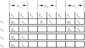
Figure 6: An instance of $\delta$A$2$LWDR corresponding to the following instance of 3DM: $T=\{\left\langle x_{1},\,y_{1},\,z_{1}\right\rangle,\,\left\langle x_{1},\,y_{2},\,z_{1}\right\rangle,\,\left\langle x_{1},\,y_{3},\,z_{2}\right\rangle,\,\left\langle x_{1},\,y_{3},\,z_{1}\right\rangle,\,\left\langle x_{2},\,y_{1},\,z_{2}\right\rangle,\,\left\langle x_{3},\,y_{2},\,z_{3}\right\rangle,\,\left\langle x_{3},\,y_{3},\,z_{3}\right\rangle\}$.

Proof:

Note that in the instance of $\delta$A$\gamma$LWDR constructed as above, clearly $\gamma=2$. We need only to show that an instance of 3DM is feasible if and only the corresponding $\delta$A$\gamma$LWDR is feasible for $K=2|X|$.

Firstly, assume that for the given 3DM instance there exists a perfect matching, say

$$M=\left\{\left\langle x_{1},\,y_{1},\,z_{1}\right\rangle,\,\left\langle x_{2},\,y_{2},\,z_{2}\right\rangle,\,\dots,\,\left\langle x_{|X|},\,y_{|X|},\,z_{|X|}\right\rangle\right\}$$

, such that no elements in $M$ agree in any coordinate, i.e. for any $l\neq l^{\prime}$, $\{x_{l^{\prime}},\,y_{l^{\prime}},\,z_{l^{\prime}}\}\cap\{x_{l},\,y_{l},\,z_{l}\}=\emptyset$ holds. Then for the constructed $\delta$A$\gamma$LWDR instance, clearly $P=y_{1},\,z_{1},\,y_{2},\,z_{2},\,\dots,\,y_{|X|},\,z_{|X|}$ is a feasible solution with $|P|=2|X|$.

Conversely, assume that $P=y_{1},\,z_{1},\,y_{2},\,z_{2},\,\dots,\,y_{|X|},\,z_{|X|}$ is a feasible solution with $|P|\geq 2|X|$ to $\delta$A$\gamma$LWDR. Then each data item in $P$ is distinct, because for every $i\in\{1,\,\dots,\,|X|\}$, $y_{i}$ and $z_{i}$ must contribute weight 2 to the total weight. That is, for any $l\neq l^{\prime}$, $\{y_{l^{\prime}},\,z_{l^{\prime}}\}\cap\{y_{l},\,z_{l}\}=\emptyset$. Therefore, $M=\left\{\left\langle x_{1},\,y_{h_{1}},\,z_{k_{1}}\right\rangle,\,\left\langle x_{2},\,y_{h_{2}},\,z_{k_{2}}\right\rangle,\,\dots,\,\left\langle x_{|X|},\,y_{h_{|X|}},\,z_{k_{|X|}}\right\rangle\right\}$ is a perfect matching for the given 3DM instance. This completes the proof. ∎

Further, the ${\cal NP}$-completeness remains true even for a very special case of $\delta$A$\gamma$LWDR :

Corollary 23.

$\delta$A$\gamma$LWDR is ${\cal NP}$-complete, even when $\gamma=2$, only three channels exist, and every item is with equal weight and appears at most 3 times in the time interval.

Proof:

It is known that 3DM is ${\cal NP}$-complete even if the number of occurrences of any element in $X$, $Y$ or $Z$ is bounded by “3” [13]. According to the transformation, because of the bound “3” on element occurrences of 3DM, both the number of channels and the occurrences of any data item can be bounded by 3. ∎

VII Performance Evaluation

In this section, we show performance evaluation of our algorithms (RFA, Algorithm 3) by experiments, and compare our algorithms with the approximation algorithm adopting maximum weight matching (MM, as in [15]) when $\delta=1$. Experimental results comparing our algorithm with an exactly algorithm (EA, based on integral linear programming (ILP)) for $\delta=2$ is also given in the appendix. We implement the algorithms using python 2.7, on a PC with Mac OS X Yosemite, 1.4 GHz Intel Core i5 processor, and 8GB 1600MHz DDR3 memory. Other than our proposed algorithm, we also implement the maximum matching heuristic, and the exact algorithm (EA). Our implementation uses the networkx library to construct both the auxiliary graphs of RFA and MM, the interior-point method of the GLPK library to solve LPs and the simplex method of GLPK to solve ILPs.

VII-A Methodology

To evaluate our algorithms, we simulate push-based broadcast programs. We denote the number of down-link channels by $m$, the total number of time slots by $T$, the total number of broadcasting data items by $N$, and the number of the packets in a request by $n$. In our experiments, $m$ is set in the range of $[2,\,16]$, $T$ in $[100,\,500]$, $N$ in $[100,\,5000]$, and $n$ in $[100,\,500]$. We assume that all the channels are with uniform bandwidth, and all broadcast data items are with the same size. Besides, for RFA, we set the value of $\gamma$ in $[3,\,50]$. In our experiments, for a given the skewed parameter $\theta$, we also assume the access probability of a data item $d_{i}$ for a request follows the Zipf distribution :

$$p_{i}=\frac{i^{-\theta}}{\sum_{i=1}^{N}i^{-\theta}}.$$

We use average download percentage (ADP) as the performance metric, and simulate 10,000 requests to get ADP for each experiment.

VII-B Experimental Results

The simulation results comparing RFA and MM are depicted in Figure 7. In all the experiments, the ADP of RFA always achieves better performance than that of MM: by about 20-32 percent in Figure 7 (a), and by about 9-20 percents in Figure 7 (b). These results are actually better than our analysis. This phenomenon is reasonable, because our algorithm is based on rounding a fractional solution of the LP relaxation of the problem. In many cases, rounding such an LP optimal solution could result in actually a much better ADP than the worst case as analyzed. Comparing Figure 7 (a) and Figure 7 (b), we find the ADP of RFA decreases when $m$ increases. That is because the problem becomes more complicated when $m$ grows, and hence the quality of the solution decreases accordingly. However, RFA still significantly outperforms MM when $m=8$, although the gap between them decreases. For the relationship between ADP and $\gamma$, as shown in Figure 7 (a) and (b), the ADP of RFA increases when $\gamma$ increases. This is consistent with our analysis of Algorithm 3: as $\gamma$ increases, $\epsilon=\frac{1}{\gamma}$ then decreases, and hence the approximation ratio $1-\frac{1}{e}-\epsilon$ increases. In particular, as we could see in Figure 7(a), ADP increases significantly from roughly 78 to 86 percents, when $\gamma$ increases significantly from 4 to 12; when $\gamma>12$, the impact of $\gamma$ over ADP grows inefficiently, i.e. ADP barely increases when $\gamma$ increases. Then ADP attains the maximum at about 88 percents at $\gamma=18$, and then ADP decreases when $\gamma>18$ grows. While $m$ is 8 instead of 2 in Figure 7(b), the weight increasing upon $\gamma$’s increment remains efficient until $\gamma>18$. Thus, for a more complicated instance, the increment of $\gamma$ benefits for a larger range.

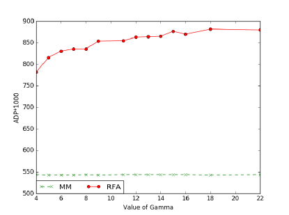
(a) $m=2$, n=400, $\gamma=2,\,\dots,\,22$.

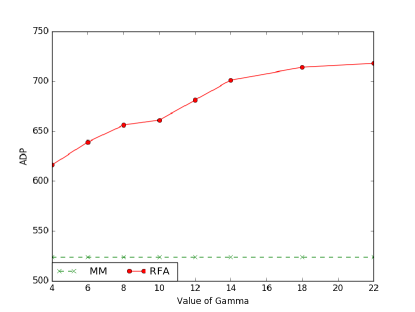
(b) $m=8$, n=1600, $\gamma=2,\,\dots,\,22$.

Figure 7: LWDR, $T=200$, $p=150$.

The simulation results on the runtime of the algorithms are as given in Table I, in which three parameters are considered: $T$, $m$ and $\gamma$, since according to our theoretical analysis in the previous section, these parameters are the factors that affect the runtime of the algorithm. In all the runtime experiments, the parameters are set $\delta=2$, $\gamma=10$ and $m=4$, where $\delta=2$ is set, since most of the mobile devices in not-long future is likely to have two antennae, provided that the current mobile devices are mostly with only one antenna. Then $m=4$ is a reasonable number of channels for $\delta=2$, while $\gamma=10$ is likely the value of $\gamma$ with best performance time ratio. Comparing the runtime of RFA and EA, we can see that the runtime of RFA is significantly lower than EA, particularly when the problem size is large, i.e. the involved $T$ is with size 500. Better still, the gap between them grows when the size of the problem increases. It is worth to note that, the time of EA is mostly the time of solving ILP, while the solver of ILP used in EA is the GLPK ILP solver, a mature package that is almost perfectly implemented. That is, with better implementation of RFA, RFA could have a runtime over EA even better than as in the table. On the other hand, we note that the runtime of RFA is higher than MM when the problem size is large. The high runtime mainly comes from the cost of solving the LP formula. When $m=4$, $T=1500$ and $\gamma=10$, the algorithm is to solve an LP of size about 20,000. However, we argue the algorithm has practical values. Firstly, the algorithm can be implemented in a better way. The current implementation is based on Python, so the runtime could be better if the algorithm is implemented in other languages such as C or C++ that is known with a better performance. Besides, the open source library GLPK that we used to solve LP, takes almost 500s to solve an LP of size 20, 000. Note that this runtime could be improved if using some other commercial libraries such as Gurobi optimizer which as claimed is more efficient than GLPK and can solve LP with up to millions of variables in a reasonable time. Last but not least, there are a lot of efficient approximation algorithms that solve LP even faster, adopting which could further improve the runtime of our algorithms. Secondly, even with our simple implementation, the average runtime of our algorithm is 500ms for LWDR with the number of request data items of 100 and a channel number of 8. Therefore, Algorithm 3 has the potential to be applied in real networks.

Table I: Runtime analysis.

Problem size of ($T,\,m,\,\gamma$)	RFA(s)	MM	EA(s)
(100, 5, 10)	0.68	0.115	1.54
(150, 5, 10)	2.22	0.245	3.07
(200, 5, 10)	4.27	0.434	6.56
(250, 5, 10)	8.03	0.655	13.10
(300, 5, 10)	13.08	0.950	19.54
(350, 5, 10)	18.54	1.27	28.08
(400, 5, 10)	25.17	1.70	38.92
(450, 5, 10)	32.48	2.09	58.56

(a)

Problem size of ($T,\,m,\,\gamma$)	RFA(s)	MM	EA(s)
(500, 5, 10)	41.34	2.60	83.79
(550, 5, 10)	54.53	3.19	117.23
(600, 5, 10)	71.46	3.75	153.37
(650, 5, 10)	89.84	4.38	214.28
(700, 5, 10)	110.67	5.07	-
(750, 5, 10)	132.80	6.60	-
(800, 5, 10)	158.78	7.42	-
(900, 5, 10)	217.22	8.35	-

(b)

VIII Conclusion

We proposed a ratio $1-\frac{1}{e}-\epsilon$ approximation algorithm for the $\delta$-antennae largest weight data retrieval ($\delta$ALWDR) problem that has the same ratio as the known result but a significantly improved time complexity of $O(2^{\frac{1}{\epsilon}}\frac{1}{\epsilon}m^{7}T^{3.5}L)$ from $O(\epsilon^{3.5}m^{\frac{3.5}{\epsilon}}T^{3.5}L)$ when $\delta=1$ [16]. To our knowledge, our algorithm is the first ratio $1-\frac{1}{e}-\epsilon$ approximation to $\delta$ALWDR for the general case of arbitrary $\delta$. To achieve this, we first gave a ratio $1-\frac{1}{e}$ algorithm for the $\gamma$-separated $\delta$ALWDR ($\delta$A$\gamma$LWDR) with runtime $O(m^{7}T^{3.5}L)$, under the assumption that every data item appears at most once in each segment of $\delta$A$\gamma$LWDR, for any input of maximum length $L$ on $m$ channels in $T$ time slots. Then, we show that we can retain the same ratio for $\delta$A$\gamma$LWDR without this assumption at the cost of increased time complexity to $O(2^{\gamma}m^{7}T^{3.5}L)$. This result immediately yields an approximation solution of similar ratio and time complexity for $\delta$ALWDR, presenting a significant improvement of the known time complexity of ratio $1-\frac{1}{e}-\epsilon$ approximation to the problem.

Appendix

A Transformation from an Approximation for $\delta$A$\gamma$LWDR to an Approximation for $\delta$ALWDR

Let ${\cal A}$ be a ratio $\alpha$ approximation with a runtime $t_{\delta A\gamma LWDR}$ for $\delta$A$\gamma$LWDR. Then a simple approximation for $\delta$ALWDR with runtime $O(\frac{1}{\epsilon})\cdot t_{\delta A\gamma LWDR}$ and ratio $(\alpha-\epsilon)$ is as in Algorithm 8.

Input: A fixed $\epsilon>0$, and an instance of $\delta$ALWDR (i.e., a set of data items to download $D=\{d_{1},\,d_{2},\,\dots,\,d_{n}\}$ with weights $w_{1},\dots,w_{n}$, together with their occurrences in channels and time slots $t_{1},\,t_{2},\,\dots,\,t_{T}$);

Output: A retrieval sequence.

1. For $i=1$ to $\left\lceil\frac{1}{\epsilon}\right\rceil$ do

      For $j=1$ to $\left\lceil\epsilon T\right\rceil$ do

         Set $t_{i+j\cdot\left\lceil\frac{1}{\epsilon}\right\rceil}$ as a vacant time slot, i.e., remove any item broadcast in $t_{i+j\cdot\left\lceil\frac{1}{\epsilon}\right\rceil}$ ;

      EndFor

      Run ${\cal A}$ against the instance and obtain a retrieval sequence $S_{i}$;

   EndFor

2. Return $S^{*}$ with $w(S^{*})$ $=\max_{i}\{w(S_{i})\}$.

Algorithm 8 An approximation algorithm for $\delta$ALWDR by transformation.

Proof of Proposition 1

Proof:

Let $OPT$ be an optimum solution to the original $\delta$ALWDR. Let $\delta$ALWDR_i be $\delta$ALWDR but with $t_{i+j\cdot\left\lceil\frac{1}{\epsilon}\right\rceil}$ vacant for each $1\leq j\leq\left\lceil\epsilon T\right\rceil$. Assume that $OPT(i)$ is the set of items in $OPT$ being set vacant. Then $OPT_{i}=OPT\setminus OPT(i)$ is an optimum solution to $\delta$ALWDR_i. Let $OPT_{i^{*}}$ be the best solution among all $OPT_{i}$s. It suffices to show $w(OPT_{i^{*}})\geq OPT\cdot(1-\epsilon)$.

From definition of $OPT_{i}$, we have

$$w(OPT_{i})\geq w(OPT)-w(OPT(i)).$$

Then

$$\sum_{i=1}^{\left\lceil\frac{1}{\epsilon}\right\rceil}w(OPT_{i})=\left\lceil\frac{1}{\epsilon}\right\rceil w(OPT)-\sum_{i=1}^{\left\lceil\frac{1}{\epsilon}\right\rceil}w(OPT(i))=(\left\lceil\frac{1}{\epsilon}\right\rceil-1)w(OPT).$$

Then

$$w(OPT_{i^{*}})\geq OPT\cdot(\frac{\left\lceil\frac{1}{\epsilon}\right\rceil-1}{\left\lceil\frac{1}{\epsilon}\right\rceil})\geq OPT\cdot(1-\epsilon).$$

This completes the proof. ∎

Following the above proof, we immediately have an approximation algorithm for $\delta$ALWDR by the transformation as in Algorithm 8.

Performance Evaluation for $\delta$ALWDR with $\delta=2$

For $\delta=2$, the experimental results comparing the performance of RFA and EA are depicted in Figure 8, where $m=2$, n=100 for Figure 8 (a), $m=8$, n=200 for Figure 8 (b), and $\gamma$ grows from 2 to 22 in both figures. The exact algorithm is to solve the integer linear programming (ILP) formula which is LP (1) but with integral $x_{i,j}\in\{0,\,1\}$. Figure 8 shows that EA performs roughly 17-30 percents better than RFA when $m=2$, and 20-35 percents when $m=8$. Since EA always produces an optimum solution, this indicates the practical ratio between the output solution of RFA and EA is better than our analysis, similar to the case in Figure 7. Besides, also like the case in Figure 7, when $\gamma$ grows the performance of RFA also gets better. The increment of $\gamma$ benefits efficiently until $\gamma=14$ in Figure 8 (a) and until $\gamma=16$ in Figure 8 (b).

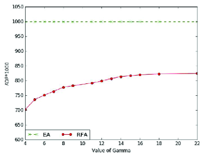
(a) $m=2$, n=100, $\gamma=2,\,\dots,\,22$.

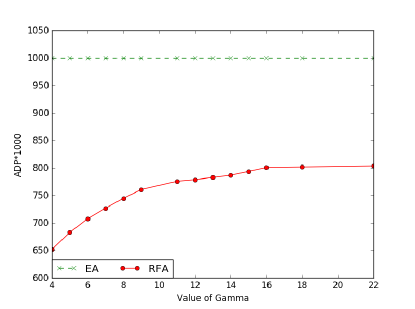
(b) $m=8$, n=200, $\gamma=2,\,\dots,\,22$.

Figure 8: $\delta$ALWDR, $T=100$, $p=150$.

References

- [1] Ashwinkumar Badanidiyuru and Jan Vondrák. Fast algorithms for maximizing submodular functions. In Proceedings of the Twenty-Fifth Annual ACM-SIAM Symposium on Discrete Algorithms, SODA 2014, Portland, Oregon, USA, January 5-7, 2014, pages 1497–1514, 2014.
- [2] Reuven Bar-Yehuda and Shimon Even. A linear-time approximation algorithm for the weighted vertex cover problem. Journal of Algorithms, 2(2):198–203, 1981.
- [3] Rong-chii Duh and Martin Fürer. Approximation of k-set cover by semi-local optimization. In Proceedings of the twenty-ninth annual ACM symposium on Theory of computing, pages 256–264. ACM, 1997.
- [4] Paul Erdös and John L Selfridge. On a combinatorial game. Journal of Combinatorial Theory, Series A, 14(3):298–301, 1973.
- [5] Uriel Feige. A threshold of ln n for approximating set cover. Journal of the ACM (JACM), 45(4):634–652, 1998.
- [6] Xiaofeng Gao, Zaixin Lu, Weili Wu, and Bin Fu. Algebraic data retrieval algorithms for multi-channel wireless data broadcast. Theoretical Computer Science, pages 1 – 8, 2011.
- [7] Michael R Garey and David S Johnson. Computer and intractability. A Guide to the Theory of NP-Completeness, 1979.
- [8] Ping He, Hong Shen, and Hui Tian. Efficient approximation algorithm for data retrieval with conflicts in wireless networks. In Proceedings of International Conference on Advances in Mobile Computing Multimedia, MoMM ’13, pages 224:224–224:233, New York, NY, USA, 2013. ACM.
- [9] Dorit S Hochbaum. Approximation algorithms for the set covering and vertex cover problems. SIAM Journal on computing, 11(3):555–556, 1982.
- [10] Dorit S Hochbaum. Approximating covering and packing problems: set cover, vertex cover, independent set, and related problems. In Approximation algorithms for NP-hard problems, pages 94–143. PWS Publishing Co., 1996.
- [11] Ali R Hurson, Angela Maria Muñoz-Avila, Neil Orchowski, Behrooz Shirazi, and Yu Jiao. Power-aware data retrieval protocols for indexed broadcast parallel channels. Pervasive and Mobile Computing, 2(1):85–107, 2006.
- [12] David S Johnson. Approximation algorithms for combinatorial problems. In Proceedings of the fifth annual ACM symposium on Theory of computing, pages 38–49. ACM, 1973.
- [13] Viggo Kann. Maximum bounded 3-dimensional matching is max snp-complete. Information Processing Letters, 37(1):27–35, 1991.
- [14] Bernhard Korte, Jens Vygen, B Korte, and J Vygen. Combinatorial optimization, volume 1. Springer, 2002.
- [15] Zaixin Lu, Yan Shi, Weili Wu, and Bin Fu. Efficient data retrieval scheduling for multi-channel wireless data broadcast. In INFOCOM, 2012 Proceedings IEEE, pages 891 –899, march 2012.
- [16] Zaixin Lu, Yan Shi, Weili Wu, and Bin Fu. Data retrieval scheduling for multi-item requests in multi-channel wireless broadcast environments. Mobile Computing, IEEE Transactions on, 13(4):752–765, 2014.
- [17] Christos Papadimitriou and Mihalis Yannakakis. Optimization, approximation, and complexity classes. In Proceedings of the twentieth annual ACM symposium on Theory of computing, pages 229–234. ACM, 1988.
- [18] A. Schrijver. Theory of linear and integer programming. John Wiley & Sons Inc, 1998.
- [19] Yan Shi, Xiaofeng Gao, Jiaofei Zhong, and Weili Wu. Efficient parallel data retrieval protocols with mimo antennae for data broadcast in 4g wireless communications. In Proceedings of the 21st international conference on Database and expert systems applications: Part II, DEXA’10, pages 80–95, Berlin, Heidelberg, 2010. Springer-Verlag.
- [20] Joel H Spencer and Joel Harold Spencer. Ten lectures on the probabilistic method, volume 52. Society for Industrial and Applied Mathematics Philadelphia, PA, 1987.