General Optimization Framework for Robust and Regularized 3D Full Waveform Inversion

Stephen Becker, Lior Horesh, Aleksandr Aravkin, and Sergiy Zhuk

1 Introduction

Scarcity of hydrocarbon resources and high exploration risks motivate the development of high fidelity algorithms and computationally viable approaches to exploratory geophysics. Whereas early approaches considered least-squares minimization, recent developments have emphasized the importance of robust formulations, as well as formulations that allow disciplined encoding of prior information into the inverse problem formulation. The cost of a more flexible optimization framework is a greater computational complexity, as least-squares optimization can be performed using straightforward methods (e.g., steepest descent, Gauss-Newton, L-BFGS), whilst incorporation of robust (non-smooth) penalties requires custom changes that may be difficult to implement in the context of a general seismic inversion workflow. In this study, we propose a generic, flexible optimization framework capable of incorporating a broad range of noise models, forward models, regularizers, and reparametrization transforms. This framework covers seamlessly robust noise models (such as Huber and Student’s $t$), as well as sparse regularizers, projected constraints, and Total Variation regularization. The proposed framework is also expandable — we explain the adjustments that are required for any new formulation to be included. Lastly, we conclude with few numerical examples demonstrating the versatility of the formulation.

2 Method and Theory

2.1 Classic Waveform Inversion

The canonical waveform inversion problem is to find the medium parameters for which the modeled data matches the recorded data in a least-squares sense (Tarantola, 1984). For linear wave equation

$$H(m)u = q,$$ (1)

where $H(m)$ is the discretized wave equation of model parameters $m$, $u$ is the discretized wavefields and $q$ are the discretized source functions. The data are then given by sampling the wavefield at the receiver locations: $d=Su+\varepsilon$, where $\varepsilon$ stands for model misspecification and measurement noise. For example, for the simplest case of constant-density acoustics in the frequency domain, the wave equation is represented by the Helmholtz operator $H(m)=\omega^{2}m+\nabla^{2}$ amended with appropriate boundary conditions, with squared slowness $m$.

The classic inverse problem can be cast as an explicit least-squares problem as follows:

$$\min_{m}\;\phi(m)=\sum_{\omega}\|\underbrace{SH(m)^{-1}Q}_{h(m)}-D\|^{2}_{F},$$ (2)

where $D=[d_{1},d_{2},\ldots d_{N}]$ corresponds to the recorded data vectors and $Q=[q_{1},q_{2},\ldots,q_{N}]$ are the corresponding source functions. $||\cdot||_{F}$ denotes the Frobenius norm which is defined as $||A||_{F}=\sqrt{\sum_{ij}a_{ij}^{2}}$.

2.2 Generalized Formulations

To accommodate robust formulations, regularizers and constraints (e.g., Eq. 4), we consider

$$\min_{y}\;\phi(y)=\sum_{\omega}\rho(h(Cy),D)+R(y),$$ (3)

where $\rho$ is a general misfit penalty, and $R$ is a regularization function, and $C$ is a linear transformation to a space of interest (e.g. Fourier, wavelet, or curvelet). Thus, the classical inversion expression (Eq. 2) is a specific case where one set $R=0$, $\rho$ as $\rho_{LS}(\hat{D},D)=\|\hat{D}-D\|_{F}^{2}$, and $C=I$ (the identity).

We provide two notable examples of $R$. In the $1^{st}$ example, we encode constraints using an indicator function $R$ that is infinite valued. Let $B$ be a closed set of feasible values of the parameters $y$, and consider

$$R(y)=\begin{cases}0&\mbox{if}\quad y\in B\\ \infty&\mbox{if}\quad y\not\in B\end{cases}.$$ (4)

The regularizer $R$ in this case is equivalent to a constraint $y\in B$, but we choose to express it as in Equation 3 because it offers a simple and uniform way to describe our algorithmic framework.

For the second example, take $R$ to be $R_{lasso}(y)=\lambda\|y\|_{1}$. This is a sparsifying penalty on the transform space coefficients $y$; the larger the $\lambda$, the faster elements of $y$ are driven to $0$. In this case, $R$ is finite valued, but not smooth. We will also use $\ell_{1}$ constraints, $R_{\ell_{1}-ball}$ defined by Eq. 4 with $B(y)=\{y:\|y\|_{1}\leq\tau\}$ for some parameter $\tau$. Projection onto this set can be performed in linear time.

The algorithmic framework we propose requires two assumptions:

1. The misfit penalty $\rho$ is differentiable. The differentiability assumption holds for least-squares, Huber (Guitton and Symes, 2003), hybrid (Bube and Langan, 1997), Student’s $t$  (Aravkin et al., 2012), generalized self-tuning extensions (Aravkin and van Leeuwen, 2012) amongst others.

2. We require that the following problem can be solved quickly (e.g., linear time in length of $y$):

   $$\hat{g}:=\operatornamewithlimits{argmin}_{g}\frac{1}{2}\|g-y\|^{2}+R(g).$$

   The vector $\hat{g}$ is known as the proximity, or prox, operator of $R$ applied to $y$, written as $\mbox{prox}_{R}(y)$.

The two examples we developed above satisfy the $2^{nd}$ requirement for the $R$. For Eq. 4, the prox operator is simply projection onto a set, which is often known in closed form. For the non-smooth $R_{lasso}$ the prox can also be implemented entry-wise, and is simply given by the soft thresholding operator $(S_{\lambda}(y))_{i}=\text{sign}(y_{i})\cdot\max(0,|y_{i}|-\lambda)$. While a closed form formula may not be available for all cases, as long as $\mbox{prox}_{R}(y)$ can be efficiently computed, our algorithmic framework applies.

2.3 Algorithmic Framework

To develop our algorithmic framework, we adopt and expand on the PQN algorithm of Schmidt et al. (2009). This algorithm was developed for optimization of costly objective functions with simple constraints. Such settings are well suited to full-waveform inversion, since function evaluations require multiple expensive forward and adjoint PDE solves. PQN builds a quasi-Newton Hessian approximation for the objective from gradient information using a limited memory BFGS scheme (Nocedal and Wright, 1999), and then solve an auxiliary subproblem

$$\min_{y}Q(y)+R(y)$$

where $Q$ is a limited memory-based convex quadratic, and $R$ represents an indicator function for simple constraints (such as Eq. 4). The subproblem is solved by the spectral projected gradient method (Birgin et al., 2000), which relies upon assumption 2 we imposed in our framework, since prox is equivalent to projection when $R$ encodes constraints.

In this study we expand this framework, allowing any function $R$ admitting an efficient proximity operator. In particular, we can then naturally incorporate sparsity promoting regularization, and total variation.

Figure 1: Gaussian (dashed black line), Laplace (dash-dotted red line), and Student’s $t$ (solid blue line); Densities (left plot), Negative Log Likelihoods (center plot), and Influence Functions (right plot). Student’s $t$-density has heavy tails, a non-convex log-likelihood, and a re-descending influence function.

3 Formulation Examples

3.1 Robust Penalties

In statistics, robust penalties are used since they penalize large residuals less than the classic quadratic norm. The Huber penalty is quadratic at the origin and becomes linear for large values of the parameter. Student’s $t$ based penalties are sublinear and have been shown to be extremely robust against outlier noise in the seismic context (Aravkin et al., 2012). Practical implementation simply requires replacement of the least-squares penalty by one of the form $\sum_{i}\log(\nu+r_{i}^{2})$, where the sum runs across a residual vector. The parameter $\nu$ can be tuned by cross validation, or using a generalized statistical formulation (Aravkin and van Leeuwen, 2012).

3.2 Sparse Regularization and Constraints

A great deal of work has underlined the importance of sparse regularization, both theoretically (Donoho, 2006; Candès and Tao, 2006) and in practice in application to seismic problems (see e.g., Herrmann et al. (2012) and references therein). Curvelets (Demanet, 2006) have been a particularly popular choice of transform space, though recent work also advocates for adaptive learning of dictionaries (Horesh and Haber, 2009). Once an efficient transform is found, $\ell_{1}$-norm solvers offer improved recovery of the parameters of interest. The non-smoothness of the regularizer is a key feature and cannot be circumvented.

4 Results

4.1 Spectral Elements Time Domain 2D Model

High-order spectral elements in the time domain over a 2D grid is used for simulation, with a test model interpolated from the SEG/EAGE salt dome model using 4 sources and 121 receivers. The $\ell_{2}$ “discrepancy” is in comparison with the test model, using the Frobenius norm, so for regularized models, it is not necessarily expected to go to zero since the test model may not be the optimal solution. The $1^{st}$ case employs the traditional least-squares loss function (Fig. 2(a)). The $2^{nd}$ uses least-squares loss with $\ell_{1}$ penalty (lasso) (Fig. 2(b)). The $3^{rd}$ test case is Student’s $t$ loss function, $\rho_{student}$, with no regularization functional $R$ (Fig. 2(d)). In the $4^{th}$ test case, we work in the curvelet domain and use $R_{lasso}$. The objective is reduced by 5 and 7 orders of magnitude, resp. (for similar initial point).

(a) $\rho=\rho_{LS}$, $R=0$

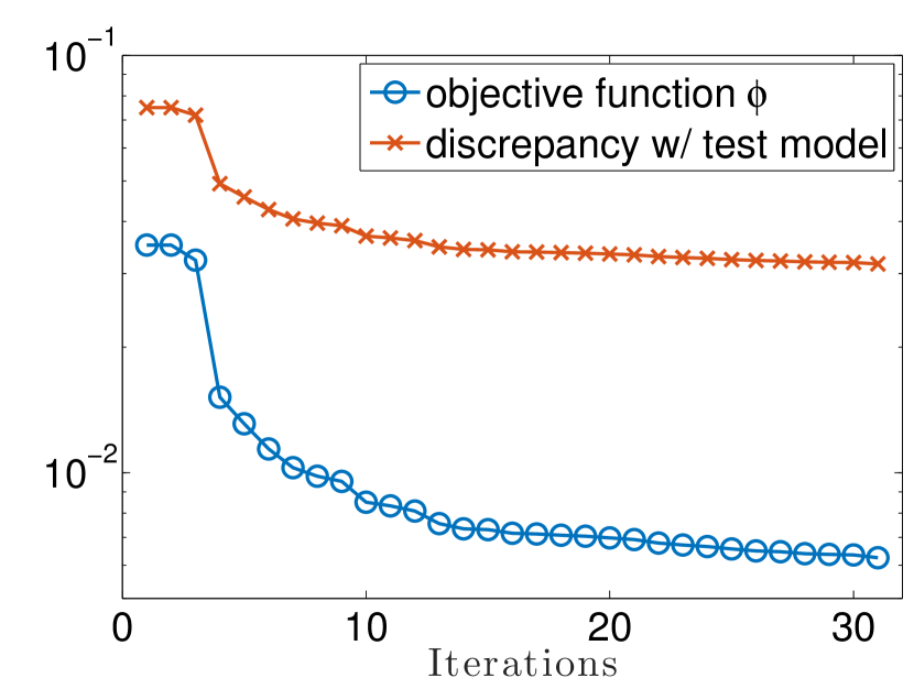
(b) $\rho=\rho_{LS}$, $R=R_{lasso}$

(c) $\rho=\rho_{LS}$, $R=R_{lasso}$ (blue), $R=R_{\ell_{1}-ball}$ (red)

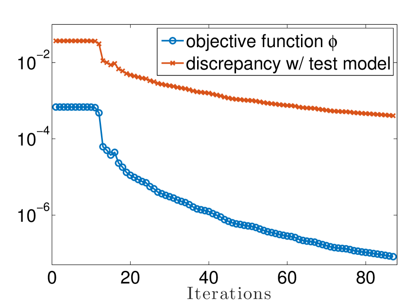
(d) $\rho=\rho_{\text{student}-t}$, $R=0$

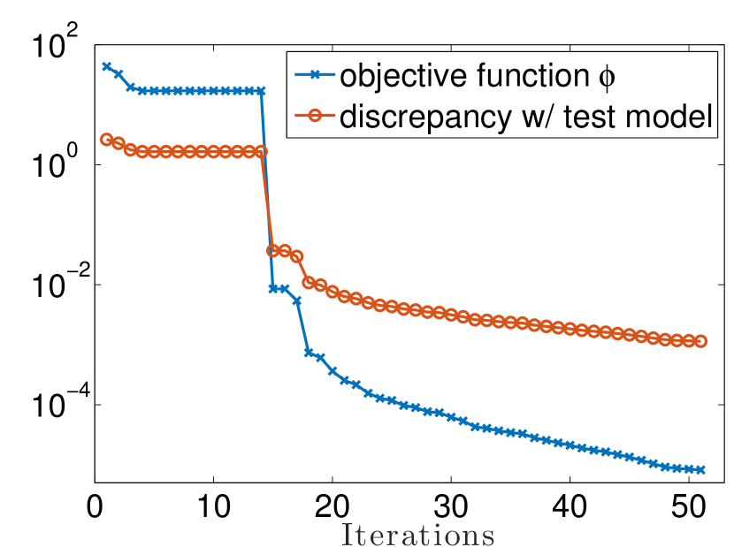
(e) $\rho=\rho_{\text{student}-t}$, $R=R_{lasso}$, $C=$curvelets

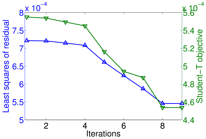
(f) $\rho=\rho_{\text{Student}-t}$, $R=0$

Figure 2: Convergence plots, for various $R,\rho,C$. $C=I$ except for (2(e))

4.2 Finite Difference Frequency Domain 3D Model

Forward simulations are performed in the frequency domain on a 3D grid. An interpolated version of the SEG/EAGE model served as the true model. Data are generated using 6 sources and 60 receivers. To validate the code, a standard least-squares inversion is performed, i.e., $\rho=\rho_{LS}$, $R=0$, $C=I$. The objective decreases by 2 orders of magnitude within 6 iterations (results not shown). The $2^{nd}$ experiment uses the same objective $\rho_{LS}$ (and $C=I$) but adds a constraint $R$ that bounds the model to be inside the $\ell_{1}$ ball of radius $\tau$. $\tau$ can be either set empirically or via cross-validation on a corpus of models. The initial iterate is set to the standard least-squares solution, so further improvement in the objective value shown on a linear scale in Fig. 2(c) is small. The $3^{rd}$ experiment is a variant of the second that replaces the $\ell_{1}$ ball with an $\ell_{1}$ penalty of strength $\lambda$, where $\lambda$ is chosen empirically but could be again tuned via cross-validation. The original PQN algorithm does not handle this case since $R$ is not an indicator function, so we modify the algorithm. In particular, we use the “Projected Scaled Sub-gradient + Active Set” solver (Schmidt et al., 2007) as the sub-problem solver. The convergence of $\rho_{LS}(h(y),D)$ is also shown in Fig. 2(c) in blue (but note that we optimized $\rho_{LS}(h(y),D)+\lambda\|y\|_{1}$ ). Finally, we switch from $\rho_{LS}$ to the Student’s $t$ based loss $\rho_{\text{student}-t}$. We show results for $R\equiv 0$ only (Fig. 2(f)), but we also have results for combining with $\ell_{1}$ ball and $\ell_{1}$ penalty terms as done for least-squares. The left-axis of the plot shows the least-squares residual, which decreases, even though this objective was not optimized.

5 Conclusions

We have presented a general algorithmic framework for large-scale FWI that offers flexible incorporation of smooth objectives, as well as various forms of regularization. The framework requires only that the proximity operator of the regularization be easily computable, which includes projections onto simple sets, as well as sparsity regularization.

References

- Aravkin et al. (2012) Aravkin, A., Friedlander, M.P., Herrmann, F. and van Leeuwen, T. [2012] Robust inversion, dimensionality reduction, and randomized sampling. Mathematical Programming, 134(1), 101–125.
- Aravkin and van Leeuwen (2012) Aravkin, A.Y. and van Leeuwen, T. [2012] Estimating nuisance parameters in inverse problems. Inverse Problems, 28(11), 115016.
- Birgin et al. (2000) Birgin, E.G., Martínez, J.M. and Raydan, M. [2000] Nonmonotone spectral projected gradient methods on convex sets. SIAM Journal on Optimization, 10(4), 1196–1211.
- Bube and Langan (1997) Bube, K.P. and Langan, R.T. [1997] Hybrid l1/l2 minimization with applications to tomography. Geophysics, 62(4), 1183–1195.
- Candès and Tao (2006) Candès, E.J. and Tao, T. [2006] Near-optimal signal recovery from random projections: Universal encoding strategies. Information Theory, IEEE Transactions on, 52(12), 5406 –5425.
- Demanet (2006) Demanet, L. [2006] Curvelets, Wave Atoms, and Wave Equations. Ph.D. thesis, California Institute of Technology.
- Donoho (2006) Donoho, D. [2006] Compressed sensing. IEEE Transactions on Information Theory, 52(4), 1289–1306.
- Guitton and Symes (2003) Guitton, A. and Symes, W.W. [2003] Robust inversion of seismic data using the huber norm. Geophysics, 68(4), 1310–1319.
- Herrmann et al. (2012) Herrmann, F.J., Friedlander, M.P. and Yilmaz, O. [2012] Fighting the curse of dimensionality: Compressive sensing in exploration seismology. Signal Processing Magazine, IEEE, 29(3), 88–100.
- Horesh and Haber (2009) Horesh, L. and Haber, E. [2009] Sensitivity computation of the minimization problem and its application to dictionary design of ill-posed problems. Inverse Problems, 25(9), 095009.
- Nocedal and Wright (1999) Nocedal, J. and Wright, S. [1999] Numerical optimization. Springer Series in Operations Research, Springer.
- Schmidt et al. (2007) Schmidt, M., Fung, G. and Rosales, R. [2007] Fast optimization methods for l1 regularization: A comparative study and two new approaches. European Conference on Machine Learning.
- Schmidt et al. (2009) Schmidt, M., van den Berg, E., Friedlander, M.P. and Murphy, K. [2009] Optimizing costly functions with simple constraints: A limited-memory projected quasi-Newton algorithm. AISTATS, Florida, vol. 5, 456–463.
- Tarantola (1984) Tarantola, A. [1984] Inversion of seismic reflection data in the acoustic approximation. Geophysics, 49(8), 1259–1266.