a \addunit\parsecpc
Likelihood-Ratio Ranking Statistic for Compact Binary Coalescence Candidates with Rate Estimation
Abstract
We present a new likelihood-ratio ranking statistic for use in searches for gravitational waves from the inspiral and merger of compact object binaries. Expanding on previous work, the ranking statistic incorporates a model for the correlations in the signal-to-noise ratios with which signals will be seen in a network of ground-based antennas while retaining an algebraic procedure for mapping ranking statistic values to false-alarm probability. Additionally, the ranking statistic enables the implementation of a rigorous signal rate estimation technique. We implement the ranking statistic and demonstrate its use including signal rate estimation in an analysis of a simulated signal population in simulated noise.
pacs:
02.50.Ey, 02.50.Sk, 02.50.Tt, 02.70.Uu, 04.30.Tv, 07.05.Kf, 95.75.Pq, 97.80.-dI Introduction
An essential ingredient of searches for gravitational waves is a statistic by which to rank candidates from least signal-like to most signal-like. The likelihood ratio (LR) has been shown to provide the most powerful detection statistic at fixed false-alarm probability Neyman and Pearson (1933), but due to technical challenges all ranking statistics used to date in searches for compact binary coalescences have been approximations of a LR. To be useful, the ranking statistic must not only be effective at ranking signals above noise, but it must not be computationally costly to implement, and there must be a known mapping from ranking statistic value to false-alarm probability.
In Biswas et al. (2012a), Biswas et al. developed theoretical aspects of the use of the LR (Winkler and Hays, 1975, Section 7.6) as the ranking statistic for searches for gravitational-waves from CBCs. For example, they showed that when a LR-based ranking statistic is used the detection efficiency is not diminished when the volume of the parameter space over which a search is conducted is increased, in contrast to techniques using other ranking statistics van den Broeck et al. (2009). That work was preceded by an earlier effort to incorporate the Virgo antenna Accadia et al. (2012) into a search for CBCs Abadie et al. (2010a), wherein the substantial difference in sensitivity of the Virgo antenna next to the three LIGO antennas Abbott et al. (2009) of the day motivated the need to explicitly account for the relative sensitivities of all antennas in the ranking statistic. Biswas et al. demonstrated an implementation of a LR ranking statistic on LIGO’s S4 data, but it was implemented as a rescaling of the traditional “combined effective signal-to-noise ratio (SNR)” ranking statistic (Biswas et al., 2012a, equation (26)), and so while the LR allowed events from times when different instruments were operating or from different regions of mass parameter space to be ranked on a common scale it otherwise provided no information not already contained in the combined effective SNR, and they continued to rely on time-shift analyses Babak et al. (2013) to map LR values to false alarm probability (FAP). In the related work Biswas et al. (2012b), Biswas et al. demonstrate the use of the LR to combine the results from several, possibly degenerate or uninformative, searches for GWs into a single unified search result.
In Aasi et al. (2013), Aasi et al. built upon the histogram-based LR ranking statistic described in Cannon (2008) for coincidences in a time-frequency burst search to develop a LR-like ranking statistic for searches for GW bursts from cosmic string cusps. Subsequently, in Cannon et al. (2013) Cannon et al. expanded upon that technique to develop an histogram-based LR-like ranking statistic for searches for GWs from CBCs, and demonstrated its use. There has also been work to approximate LR ranking statistics using space-partitioning decision trees in searches for GW bursts Adams et al. (2013), and in CBC searches Baker et al. (2014); in the latter the mapping from ranking statistic to FAP was accomplished through the use of time-slides while in the former the ranking statistic was applied to gamma-ray burst (GRB)-triggered searches and the mapping was constructed using on-source/off-source comparisons. In contrast, the ranking statistic developed in Cannon et al. (2013) had the property that if applied to the candidates collected from a search pipeline possessing certain simplifying characteristics, it was possible to compute the mapping from ranking statistic to FAP algebraically.
The ranking statistic in Cannon et al. (2013) was an approximation of the LR in which it was assumed that the characteristics of a signal-like event in one instrument were independent of that same event’s characteristics in other instruments — that the probability density function (PDF) in the ranking statistic’s numerator could be factored into a product of single-instrument terms. This approximation simplified the software needed to implement the ranking statistic and afforded a simple numerical integration scheme for computing the FAP for any value thereof.
Although the ability to compute FAPs algebraically was a significant improvement over previous techniques, three limitations remained. (i) The ranking statistic assumed the SNRs at which a signal is observed in the various instruments are independent random variables. For low SNRs where plausible early detections are expected this is a good approximation but for higher SNRs this approximation yields a less-than-optimal ranking statistic in that it does not properly penalize candidates with implausible SNR combinations that have resulted from, e.g., non-stationary noise in one detector. (ii) No attempt was made to include within the ranking statistic knowledge of which instrument combination had identified the candidate, leading to a unique ranking statistic scale for each combination of instruments, something the work of Biswas et al. had already addressed. (iii) Finally, although the FAP for each value of the ranking statistic could be computed, with only an approximate PDF for the numerator a true-alarm probability (TAP) (probability of at least one candidate at or above a given value of the ranking statistic given the presence of a signal) could not be computed which excluded the possibility of combining the ranking statistic with the rate estimation technique of Farr et al. Farr et al. (2013).
Here, we address these limitations by showing how to compute and incorporate the probability of observing signals and noise events in various combinations of instruments into both the numerator and the denominator, and how to incorporate the joint PDF for the SNRs in the numerator. These modifications will require us to abandon the use of explicit numerical integration for computing the ranking statistic PDF in signal-free data — the first step in mapping ranking statistic values to FAPs — and switch to an importance-weighted sampling procedure, the details of which will also be explained.
II Example
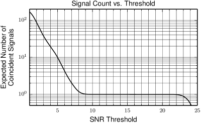
To demonstrate the application of the ranking statistic, we have performed a test analysis of about of stationary Gaussian noise simulating the Advanced LIGO and Virgo antennas and possessing the spectral densities described as the “early” noise curves in Barsotti et al. (2012); van den Broeck (2013). A population of binary neutron star (BNS) merger events was injected into the data from a population of sources distributed uniformly in volume to a distance of , uniformly in component masses in the range –, with Gaussian-distributed dimensionless spins centred on 0 with a standard deviation of 0.4 a cut-off of 0.7 and isotropic orientations, and occurring at a mean rate of . This is not meant to be astrophysically realistic Abadie et al. (2010b), but to provide a useful sample of detectable signals. Comparing the injected waveforms to the noise spectra and accounting for the relative orientations of the antennas and the sources at the time of each simulated event, one can determine the SNR at which the signal should be seen in each antenna, and from that estimate how many signals should be seen in two or more antennas (i.e., form a coincident candidate event) as a function of the single-detector SNR threshold applied. This is shown in FIG. 1.
The data was filtered using a template bank consisting of 6278 non-spinning BNS waveforms with component masses in the range –, and having a minimal match of 0.975 (with respect to the template family). The template bank was laid out using the lalapps_tmpltbank program from the LALSuite software package Aasi et al. , and candidate events collected using the gstlal_inspiral program from the GstLAL software package Cannon et al. ; Cannon et al. (2012). The plots and results shown in what follows are taken from this analysis.
III Ranking Statistic,
The ranking statistic is the LR
| (1) |
where is the set of horizon distances for all instruments in the network at the time the event is observed (see Appendix A), is the specific set of instruments in which the event has been observed, and are the template matched-filter SNRs and values (Allen, 2005, and references therein) for the candidate in each of those instruments, and are the intrinsic parameters of the template. The time at which the event is observed enters implicitly through the horizon distances which fluctuate in time as environmental factors and operating conditions at the observatories change; in fact, is best thought of as simply a clock, and since time influences the distributions of other parameters through their dependence on the (time-dependent) instrument sensitivities, the labelling of times on the clock is most conveniently done with the instrument sensitivities themselves. We’ll say a few more words about the time dependence and the ranking statistic below. The template’s intrinsic parameters, , can be a label identifying a template in the search, or identifying a group of templates if that is found to be convenient. Anticipating what follows, we have factored out of the PDFs on the right-hand side of (1). For brevity we will drop from the notation in the remainder of Section III; it should be remembered that we will be deriving PDFs for a choice of .
The differences between the times at which the event is observed at each location on Earth are not used, nor are the phases with which the waveforms are recovered at each observatory. These omissions are an obvious avenue for future improvements but, for signals, the inter-antenna time delays and waveform phases are correlated with the SNRs and their inclusion would make the numerator substantially more difficult to compute numerically.
We factor the numerator of the fraction in (1) as
| (2) |
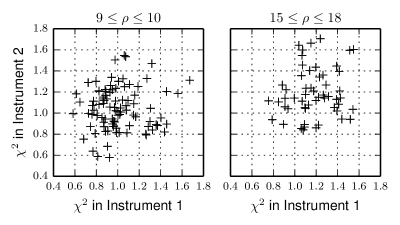
That is, we write it as the probability of the collection of instruments having some given sensitivities multiplied by the probability that a (detectable) signal is visible in a set of those instruments (and no others) given the sensitivities of all instruments multiplied by the joint probability density of the SNRs in that set of instruments multiplied by the product of the probability densities for the values given the SNRs and the instruments. In particular, we assume here that except for their correlation with SNR the values observed in different instruments for the same event are statistically independent random variables, i.e., that the residual from which the is computed is dominated by instrumental noise and not by systematic waveform errors (which would be common to all instruments in the network). The validity of this assumption can be checked visually with scatter plots like those shown in FIG. 2.
We assume the noise processes in the different instruments are statistically independent of each other and independent of the sensitivity of the antennas to GWs and so the denominator of the fraction in (1) can be factored into several low-dimensional terms.
| (3) |
The factor is common to the numerator and denominator and, so, for the purpose of evaluating the horizon distances appear only parametrically and only in the numerator. Later, when using the numerator and denominator to map values to FAP and TAP the factor will be included in those integrals. Since we understand to be the labelling of a clock, . In the following subsections we show how each of the remaining terms in (2) and (3) is obtained.
III.1
To obtain the probability that a signal yields coincident above-threshold events in exactly some combination of instruments, we begin by assuming that the coincidence time window is sufficiently large that if a signal is seen above the SNR threshold in two instruments the threshold crossings will occur within that pair’s coincidence window with certainty. This assumption is essentially equivalent to requiring the coincidence window for each pair of instruments to be at least as large as the sum of their reciprocal bandwidths plus the light travel time between them (at most few tens of milliseconds for ground-based laser interferometer antennas). If a more sophisticated ranking statistic is considered in the future in which the time-of-arrival of the events in each of the instruments is treated more carefully than to simply construct a pass/fail test, or if the coincidence window for the pass/fail test is small, then this assumption would need to be revisited.
Given our assumption about the formation of coincidences, we need only consider the probability that the signal is seen above the SNR threshold. The probability that a detectable signal is visible in exactly some collection of instruments, , (and no others) can be obtained to satisfactory accuracy by Monte Carlo integration. Referring to Appendix A, a uniformly-distributed source position is selected on the sky and the antenna responses to the and polarizations computed, the cosine of the orbit inclination is drawn uniformly from , and from the antenna responses and orbit inclination the quantity is computed for each instrument in the network using (16). The number of sources visible above the SNR threshold in two instruments whose sensitivities are characterized by and is
| (4) |
while the number of sources visible to two instruments and not a third is
| (5) |
and so on. All of these integrals diverge for the same reason that (18) diverges: as . The probabilities that we seek will be the ratios of sums of integrals like (4) and (5), and even though the integrals diverge it might be the case that the ratios we seek are well-defined; or it might be that the ratios can be made to be well-defined by introducing a regularization, possibly one derived from the constraint that we seek a ranking statistic to extremize detection efficiency at fixed false alarm rate (FAR).
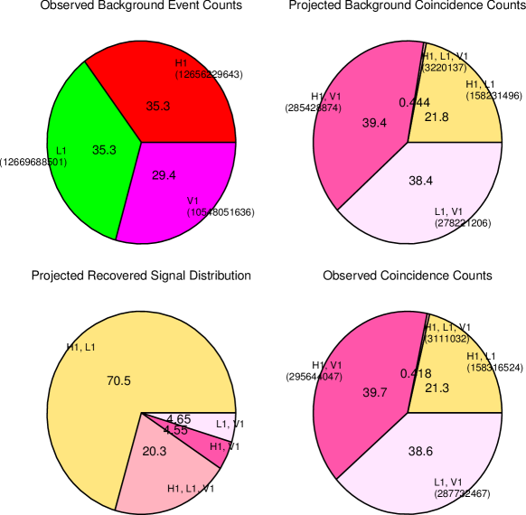
Unfortunately we have not been able to make progress in this direction. Instead, we proceed as follows. We take (19) to give the rate (up to an irrelevant constant) at which signals in the given direction and with the given polarization and given orbit inclination are seen by each instrument in the network, and then assume that all signals visible to the least sensitive instrument are visible to the next least sensitive instrument with certainty, and so on. This works best if the instruments are not all very similar in sensitivity, which is likely to be the case as the network of ground-based GW antennas is commissioned in a staggered schedule. With that assumption, from differences and ratios of the rates one can compute the probability that a source will be visible to some combination of instruments (and no others) assuming that it is visible to at least two. These probabilities are added to a histogram and the process of selecting a sky location and so on is repeated. When sufficient iterations have been made, the histogram is normalized. We find that after 500,000 iterations the variance of the result is reduced to one part in , and a Python implementation of the sampling loop using antenna response code implemented in C in LALSuite Aasi et al. completes in about on typical modern hardware. An example for is shown in the bottom-left panel of FIG. 3.
III.2
The calculation of the joint PDF of the SNRs involves the same framework as was used in Section III.1, and encounters some of the same difficulties. The PDFs are computed using Monte Carlo integration of the density at each site in a multi-dimensional SNR histogram. Each axis is binned using an binning as described in Appendix B. Referring to Appendix A, a uniformly-distributed direction is selected on the sky and the antenna responses to the and polarizations computed, the cosine of an orbit inclination is drawn uniformly from , and from these the quantity is computed for each instrument in the network using (16).
We identify the most sensitive of the instruments that must see the source, and step through a sequence of bins of nominal SNR, , in that instrument. Each bin has a lower bound, an upper bound, and a central value. From the ’s and each bin’s central value, the in all other instruments are computed. With respect to the instruments that must not see the signal, we make the assumption that if the nominal SNR in those instruments is below the detection threshold, , then they are all blind to it with certainty, and if above in one of them it sees it with certainty. We are approximating the Marcum Q-function with a Heaviside function for performance purposes, and will rely on the superposition of many trials combined with a convolution of the histogram with a density estimation kernel to hide the approximation. The binning of in the most sensitive instrument is started at 1, and terminated when this latter condition is met. Using (16) and in the most sensitive instrument, the lower and upper bounds of each bin can be converted into upper and lower bounds, respectively, on the physical distances of the corresponding sources. The number of sources in the bin is proportional to the difference of the cubes of these, see FIG. 4.

The SNR PDF is computed by iterating over the binning, at each bin computing a vector of Rician-distributed random variables having noncentrality parameters given by the bin centre’s co-ordinates to give a vector of observed SNRs, and adding to that location in the binned PDF. A new sky location, etc., is chosen and the whole process is repeated. Note that this procedure results in each bin in the SNR PDF containing a number proportional to the rate of signals in that bin, not the PDF in that bin.
After a satisfactory number of iterations has been completed, the array of signal rates is convolved with a Gaussian density estimation kernel, all bins below in any instrument are zeroed, and the array divided by its sum (so that its sum is 1). Finally each bin is divided by its volume in SNR to yield the properly-normalized PDF. Examples of PDFs obtained this way are shown in FIG. 5.
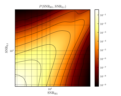
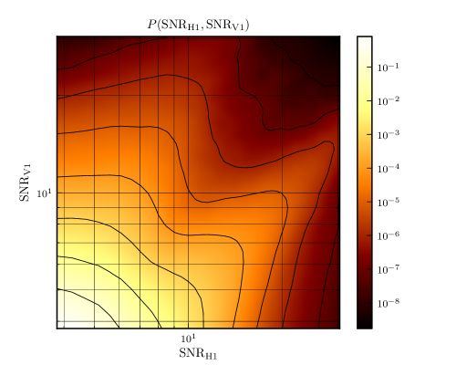
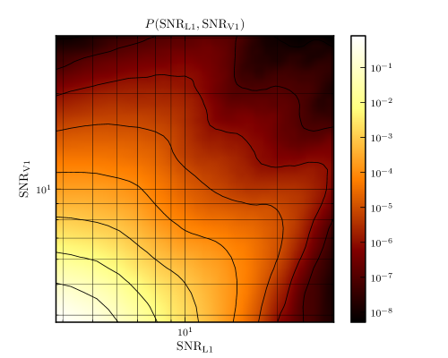
For these, the binnings along each axis are given by , , , 80,000 iterations of the outer sky-location loop were performed, and a Gaussian density estimation kernel with a standard deviation of 1.875 bins was employed.
III.3
We begin by obtaining as described in Cannon et al. (2013), using an analytic expression obtained by assuming recoverable signals are to be found in glitch-free, Gaussian, noise. As before, the implementation samples the PDF on a discrete rectangular grid of vs. in order to better fit the natural shapes of the PDF’s contours to the rectangular grid of bins. For both the and axes we now use the binnings described in Appendix B. The axes are binned using , , ; the axes using , , .
Once that PDF is obtained, columns of constant are renormalized so that their integrals are 1, converting the function represented by the array from a two-dimensional density to a 1-dimensional density in parameterized by .
III.4
The search algorithm employs a bank of two-phase matched filters applied to the strain time series recorded from each of the instruments. When the magnitude of the output of a filter crosses a preset threshold, , a peak finder identifies the sample with the highest SNR, and that point in that filter’s output is recorded as an event, (sometimes called a “trigger”, borrowing language from particle experiments). A “coincidence” occurs when two or more instruments register events from the same filter within some window of time, , where and are the positions of the two antennas and is the speed of light. When more than two instruments participate in the coincidence all time differences between pairs of events in the coincidence must satisfy the respective constraints.
There is a maximum rate at which events can be recorded (for example, limited by the sample rate of the time series), but this limit is much higher than the mean rate and so in the absence of signals the number of events recorded in some interval from one filter is adequately approximated as a Poisson process. After measuring the mean rate of events in a filter in each instrument, say by counting the number collected over some large interval of time, it is straightforward to use the single-instrument rates and the coincidence windows to compute the rates at which coincidences will occur between pairs of instruments. For example, if two instruments yield events at mean rates and , and the coincidence window is , the mean rate at which coincidences occur is
| (6) |
because is the number of events in instrument 1 per unit time, and is the number of events in instrument 2 one expects to find within of each of them.
Computing the rate at which higher-order coincidences occur is non-trivial, and we do so using a stone-throwing technique. For example, to compute the rate at which triple coincidences occur, we start by computing
| (7) |
giving the rate at which events in instrument 1 are found in coincidence with events in both instruments 2 and 3. The rate at which 3-way mutual coincidences occur is
| (8) |
where is the probability that events in instruments 2 and 3 are found to be in coincidence given that they are both known to be coincident with an event in instrument 1. This probability is computed by stone throwing: uniformly-distributed time differences are chosen for instruments 1 and 2 and for instruments 1 and 3, both consistent with the coincidence criteria for those pairs; the time difference between 2 and 3 is computed from these and if it satisfies the coincidence criterion for that pair a successful outcome is recorded; the ratio of successful outcomes, , to total trials, , converges to the desired probability as the number of iterations increases. The number of successful outcomes is a binomially-distributed RV with standard deviation where is the probability of success (Winkler and Hays, 1975, Section 4.3). We iterate until the ratio of the upper bound of the standard deviation of the number of successes to the observed number of successes, , falls below some tolerance
| (9) |
This stopping criterion requires a minimum of iterations before it can be met. The number of iterations required, beyond that, is minimized by choosing “instrument 1” to be the instrument for which the Cartesian product of the coincidence windows between it and the other instruments is smallest, so that coincidence with that instrument provides the tightest prior constraint on the time differences among the other instruments, and the rate of successful outcomes is maximized.
When some combination of instruments yields mutually coincident events, it is possible those events are also coincident with an event in some other instrument. The rate at which coincidences occur that involve some combination of instruments and no others can be found by subtracting from that instrument combination’s coincidence rate the rates of coincidences of all proper supersets of that combination. For example, if the network consists of three instruments, the rate at which exactly instruments 1 and 2 are coincident is
| (10) |
where because there are no other instruments. Having obtained, for each instrument combination, the rate at which coincidences occur involving those instruments and no others, the probability that a coincidence chosen at random involves exactly some combination of instruments is obtained by the ratio of each such rate to the sum. For example, in the three-instrument case,
| (11) |
An example of the result with , and a comparison of the predicted to the observed behaviour is shown in FIG. 3.
III.5
This PDF is obtained exactly as described in Cannon et al. (2013), by histograming the properties of single-instrument events that fail to be coincident with events in any other instruments. As before, the implementation uses a histogram binned on a rectangular grid in vs. in order to better fit the natural shapes of the PDF’s contours to the rectangular grid of bins. For both the and axes we now use the binnings described in Appendix B.
III.6
In considering the Bayes factor for the intrinsic parameters of a candidate, , we first point out that in the example implementation, a “coincidence” is formed when two or more instruments in the network register events from the same filter within some window of time. Therefore, there is no distinction between the carried by single-instrument events and the carried by a coincidence. Searches for GWs using algorithms that permit a waveform mismatch between instruments in a coincidence will require a different technique for computing the Bayes factor for than presented here.
The denominator, , is obtained as a by-product of the procedure in Section III.4 for obtaining . Recall that for brevity we have been omitting from the parameters of the PDFs, and that (11) was implicitly for a choice of . The denominator in (11) gives the total rate of background coincident events expected for a choice of . is obtained by dividing that rate by the sum of those rates for all .
is chosen by the individuals performing the search. Specifying the relative frequency at which templates are expected to yield candidates as a result of genuine signals is how the ranking statistic is informed of ones prior belief about the distribution of the intrinsic parameters carried by signals of astrophysical origin. In the example implementation demonstrated here, was chosen to be uniform on the manifold in waveform space comprising the template bank, i.e., all templates are considered equally likely in the signal population. This prior is the one implicitly chosen in past searches for GWs from CBCs. Because the waveform space’s metric is determined by the noise spectrum of the antennas, i.e., not by the physical properties of the sources, this prior is not uniform in any astrophysically meaningful quantities, like the mass of the source. Other choices might be better in future searches. One could conceivably fix to be uniform in template index, and vary the template density to affect the desired prior in astrophysical parameters. This is the most computationally efficient as it avoids, maximally, the filtering of templates whose events are subsequently discarded by the ranking statistic, but one needs to be certain of the choice of prior in advance because the SNR lost in low-density regions of the template bank cannot be recovered without re-analyzing the data if one decides that a different prior is desired. Although searches for CBCs have not done so, template-based searches for cosmic string bursts Aasi et al. (2013) and for continuous waves from pulsars Jaranowski et al. (1998) do incorporate astrophysical priors into their template weighting and/or placement.
III.7 Time Dependence
As discussed above, we have constructed a framework that allows us to include the time dependence of the antenna noise floors (encoded via horizon distance) in the ranking statistic. The daily cycle of human activity, weather, and thermal changes to optics can alter the Gaussian noise floor of the antennas substantially on time scales of hours, these changes are easily tracked on time scales of minutes, and so there is both a desire and an opportunity to incorporate knowledge of Gaussian noise floor fluctuations in the assessment of candidates on an event-by-event basis.
Other quantities change in time as well. The mean background event rates change, and the antennas undergo periodic maintenance that can alter the statistical properties of their noise processes, for example changing the distribution of parameters. We do not explicitly include the time dependence of these other quantities in the description of the ranking statistic given here. In practice it is found that a week or more of data is required before the histograms used to model the noise PDFs in the ranking statistic’s denominator have converged enough that the ranking statistic value assigned to a given candidate is, effectively, stable. Therefore it is not possible to monitor or even define changes to these PDFs on time scales less than .
At the same time, to simplify the management of the computer systems, one tends to analyze data in blocks of time, and these blocks tend to be of about the same duration as is required to stabilize the denominator PDFs. Therefore, through this piecewise analysis of the data, by simply collecting fresh histograms within each block of time the time dependence of, for example, the histograms, is naturally incorporated into the ranking statistic. Finally, as was done in Section III.4 to normalize the ranking statistic across different instrument combinations, recording the mean background event rate in each interval of time allows the ranking statistic to be normalized across disjoint analysis blocks providing a single, unified, ranking statistic for the entire experiment.
IV False-Alarm Probability
We now have all the ingredients of the ranking statistic, and so at the end of a search for GWs from CBCs we can order the candidate events from most signal-like to least signal-like. We wish to know how significant a discovery the most signal-like of the candidates are: should we have expected to see things so signal-like by random chance from the noise, or might these be genuine signals? To accomplish this, we require
| (12) |
the PDF for (for a choice of intrinsic parameters) in the noise population. This is obtained by integrating the noise PDF for all parameters in the ranking statistic over dimensional surfaces, , of constant . The complementary cummulative distribution function (CCDF) of (12) gives the probability that a noise event drawn at random is found to have a value of at least as high as some threshold, and from that one can obtain the probability that a signal-free experiment of some duration (that yields some number of events) yields one or more events with values of at least as high as some threshold — the FAP. The details of this were discussed in Cannon et al. (2013), here we will describe how (12) is evaluated in the context of the new expression for .
We do not know the surfaces of constant , instead we construct an approximation of by visiting points in the -dimensional parameter space, evaluating and at each point that we visit (“” are the -dimensional co-ordinates of the point), and constructing a histogram of with each sample weighted by . As explained in Section I, in Cannon et al. (2013) the approximation of the LR as a product of several low-dimensional terms allowed this sampling procedure to be performed by exhaustively visiting every point in the discretely-sampled PDFs. Because, here, the numerator of no longer factors into independent single-instrument terms we can no longer use this technique, exactly. Instead of factoring and exhaustively evaluating it at each grid point in the single-instrument PDFs, we leave it as an -dimensional function and evaluate it at a randomly-selected subset of grid points in the -dimensional space, and histogram those results alone. As the number of samples gets large the histogram of samples converges to . The rate of convergence can be increased by adjusting the PDF from which grid points are drawn (and re-weighting the samples appropriately). This technique for approximating integrals is known as importance-weighted sampling (Landau et al., 2007, Section 11.7.2).
The total number of distinct -dimensional grid points in the binning used to represent is enormous — in our example it’s over — but we find that a satisfactory approximation of the PDF can be obtained after just samples. The result is shown in FIG. 6.
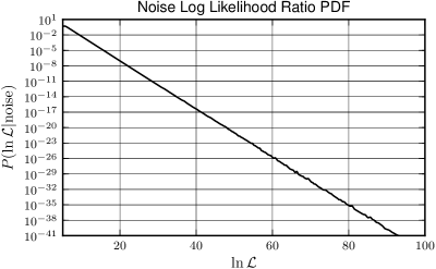
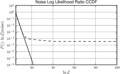
This was obtained using an binning for as described in Appendix B with , , and . All indexes for the binnings comprising the space over which is defined were drawn from uniform distributions except the bins whose indexes were drawn from a distribution whose cummulative distribution function (CDF) is proportional to and restricted to bins not below the single-instrument SNR threshold, . This distribution was arrived at empirically to efficiently favour interesting SNRs. The counts in the histogram were convolved with a Gaussian density estimation kernel having a standard deviation of 8 bins, the array of counts then rescaled so that its sum was 1, and then each bin divided by its size in to yield a normalized, discretely-sampled, PDF.
Note that the PDF and CCDF have been truncated at . The procedure by which candidate events are collected employs a clustering step to remove redundant candidates resulting from each signal. It has been found that above the noise process yields candidates at a sufficiently low rate that their population is unaffected by the clustering. Modelling the PDF for the noise process below requires the clustering process to be taken into consideration, and this will be the subject of future work. The remainder of the procedure for converting into a mapping from to FAP and FAR is exactly as in Cannon et al. (2013), and without the clustering model is applicable only above the cut-off threshold of .
V Event Rate Estimation
Since we have a reasonable model for in the numerator of , the procedure described above for approximating (12) can also be used to approximate by replacing in the integrand with . In fact, the exact same procedure is used, and approximations of both and are obtained simultaneously in the same sampling loop. Following through with a marginalization over yields . An example is shown in FIG. 7, where both the PDF and CCDF have been truncated at to match what was done with the noise model.
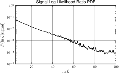
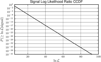
and are the ingredients required to implement the signal rate estimation technique of Farr et al. Farr et al. (2013). Farr et al. derive the joint PDF for the rates of signal events and noise events from the ranking statistic values assigned to all events collected in the experiment, (Farr et al., 2013, equation (21)). Marginalizing this PDF over background rate yields the posterior PDF for the rate of signals during the experiment. Farr et al. imply the possibility of obtaining a closed-form expression for this posterior, but for experiments with a large number of candidate events we find that approach to be intractable. We resort to Markov chain Monte Carlo sampling from the joint PDF for the marginalization. For this we use the emcee sampler by Foreman-Mackey et al. Foreman-Mackey et al. (2013).
We wish to obtain credible intervals from the signal rate posterior PDF. In particular, we wish to know if the credible interval excludes 0. To achieve this, we need to measure the posterior’s tails well, and running the sampler long enough to do so using the correct PDF is inconvenient. Therefore, we sample from the square root of the joint PDF given in (Farr et al., 2013, equation (21)), and correct the histogram of samples by squaring the count in each bin and dividing by the bin size. An example of the result is shown in FIG. 8.
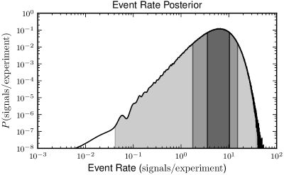
This was obtained with 40 walkers, the chain burned-in for 1,000 iterations, then run for 400,000 iterations, and the samples histogrammed using a uniform-in-logarithm binning spanning the range of values returned from the sampler and having about 22,000 bins (so there is an average of about 730 samples per bin). Implementing the posterior function in C and parallelizing the sum within it using OpenMP, the sampling process takes several hours on a modern 16-core machine. After correcting the bin counts as described above, the corrected counts were convolved with a Gaussian density estimation kernel having a standard deviation of 5 bins, the convolved bin counts normalized to have a sum of 1, and finally divided by the bin sizes to yield the normalized discretely-sampled estimate of the posterior PDF.
The mean of the signal rate posterior PDF in the example is , the maximum likelihood signal rate is , the 68% credible interval is , the 95% credible interval , and the 99.9999% credible interval is which, in particular, excludes 0. In our example analysis, we have the benefit of knowing the list of synthetic signals that were added to the data, and we can consult that list to see how many of them are expected to be visible above the SNR threshold in at least two instruments. That number as a function of the SNR threshold is shown in FIG. 1. The example analysis used a single-instrument SNR threshold of , and apparently 19.4 signals are expected to have yielded candidate events involving a coincidence between at least two instruments. Additionally, as discussed above, to remove the need to model clustering survival, a ranking statistic cut has been imposed discarding all events with . Of the 19.4 signals expected to yield coincident events, only 11.5 are expected to survive the ranking statistic cut.111This is arrived at by drawing SNR and values from distributions constructed for each injection, evaluating the ranking statistic at those values, and measuring the survival probability for each injection by iterating. That analysis indicates that 12.1 signals are expected to survive all cuts, but at the ranking statistic threshold the clustering is already causing about 5% of events to be lost so we suppose that 0.6 more events are lost due to clustering and conclude that about 11.5 should remain. This rate of signals is within the 75% credible interval, and so there is already reasonable agreement between the posterior PDF and the known expected signal rate, but it is also possible that a bias is present. In considering the origin of a bias, our simple choice of does not correspond to the probabilities with which signals are expected to be recovered by different templates, and some bias is to be expected as a result of this. Probably the dominant reason for a bias, however, is that the injected signals were drawn from a population of sources with spinning components whereas the templates used to identify candidates were non-spinning and therefore would not have recovered as much SNR as they could have, and even small losses can significantly impact the expected rate. For example, assuming the mismatch due to spin results in an average loss of SNR of just 6% reduces the expected signal recovery rate to , which is within the 50% credible interval, and in essential agreement with the posterior PDF. A detailed investigation of the SNR recovery efficiency of the template bank used in the example search is beyond the scope of this work; the naive assumption that the template bank efficiency is given by the template bank’s density already yields good agreement between the posterior PDF for the signal rate and the signal population, and so if there is a bias in the signal rate posterior it is not greater than can be explained by assuming a few percent loss of SNR.
VI Conclusion
We have shown the construction of a new ranking statistic for searches for GWs from CBCs, and demonstrated its implementation including an exposition of the technical details required to do so. We have shown that the ranking statistic continues to allow us to construct a mapping to FAP without the use of time slides. We have shows that the ranking statistic can now be used with the rate estimation technique of Farr et al. Farr et al. (2013) to obtain a reasonable posterior PDFs for the rate of signals observed during an experiment. We have found that while the identification of single, statistically-significant, outlier is not adversely affected by small SNR losses arising from signal/template mismatch, the inference of a signal rate from the population of candidate events collected by the analysis can be sensitive to small SNR losses due to template bank inefficiency. This is not unexpected since the rate of detectable signals should scale cubically with the SNR collected by the templates, and we showed how adjustments to the expected rate of recovered signals resulting from as little as a 6% SNR loss in the template bank can bring the measured signal rate posterior PDF into good agreement with the population of signals we know to be in the test data.
Future work will look more carefully at the problem of interpreting the signal rate posterior PDF in terms of an astrophysical merger rate. In particular, we will examine the problem of modelling the loss of low-significance events due to clustering in more detail, and incorporate a more detailed analysis of the SNR recovery efficiency of template bank in the interpretation.
Acknowledgements.
KC and JP were supported by the National Science and Engineering Research Council, Canada. This work has LIGO document number LIGO-P1400175. We thank the UW-Milwaukee Center for Gravitation and Cosmology and the LIGO Laboratory for use of its computing facility to make this work possible through NSF grants PHY-0923409 and PHY-0600953. We thank the LIGO Scientific Collaboration and the Virgo Scientific Collaboration for providing us with the data to test the methods described in this work. Figures were generated with Matplotlib Hunter (2007). KC thanks Jolien Creighton for his careful reading of the manuscript and many helpful insights that have improved the efficiency of the implementation of the techniques described herein, and thanks Ilya Mandel for his assistance improving this presentation of our results. All remaining problems are our own.Appendix A Distance and SNR
For convenience, we collect here some relationships relating the distance to a GW source, its SNR, and the number density of sources.
The strain seen in a GW antenna is the projection of the GW field onto the antenna’s response tensor, and in terms of the two transverse, traceless, polarization components of the field, and , can be written (Thorne, 1987, Section 9.4)
| (13) |
where the antenna response factors, and , depend on the direction to the source, , and the orientation of the polarization axes, (Anderson et al., 2001, equation (B6)). For non-precessing CBCs whose radiation is dominated by the mode, is inversely proportional to the effective distance (Allen et al., 2012, equation (3.3c))
| (14) |
where is the physical distance to the source, and the angle between the line-of-sight to the source and its orbital axis. , and a source is “optimally oriented” with respect to an antenna when .
Defining to be the nominal matched-filter output observed for a signal in the absence of noise, Allen et al. (2012). This relationship can be written as
| (15) |
thereby defining , the “horizon distance”, the physical distance at which an optimally-oriented source is seen with a nominal SNR of 8 Allen et al. (2012). Note that depends on the antenna noise spectrum and the physics of the GW source: one may speak of an horizon distance being associated with a source by assuming a canonical antenna noise spectrum, or with an antenna by assuming a canonical source; stronger emitters of GWs are said to have larger , less sensitive antennas smaller . Combining (14) and (15),
| (16) |
where the parameter is introduced for compactness: a sort-of “noise-limit distance”, the physical distance at which a source with the given geometric arrangement with respect to a given antenna is seen at an SNR of 1 in that antenna.
In stationary Gaussian noise the SNR, , at which a signal is recovered is a 2 degree-of-freedom (DOF) noncentral -distributed RV with noncentrality parameter (Allen et al., 2012, Section IV). This is also known as the Rice distribution with and noncentrality parameter (Rice, 1945, equation (3.10-11)).222Reference is to Rice’s original work; he does not call the distribution by that name. The probability that a source with nominal SNR is observed above some SNR threshold is
| (17) |
where is the first-order Marcum Q function Marcum (1960). Assuming the number density of sources to be uniform in volume, it is , therefore the total number of sources in a given direction with a given polarization and orbit inclination visible to an antenna with a given horizon distance is
| (18) |
Because the integral diverges. Physically, assuming a uniform source density to arbitrary distance yields an infinite number of sources at infinite distance with zero nominal SNR that, nevertheless, due to noise fluctuations have a non-zero probability of registering as events. Because the universe has a finite age and stellar evolution must be allowed to progress for a period of time after the birth of the universe before compact object mergers can occur, the source density must, really, fall to 0 at some distance, and if this is correctly accounted for this integral must be finite — Olbers’ paradox revisited.
If the number density cutoff occurs at a distance (the antennas cannot see as far as the first sources), then the integral in (18) becomes a function only of the signal detection threshold, , and taking that to be a fixed parameter we can side-step the divergence and say
| (19) |
Appendix B Binning
In implementing the ranking statistic described in this article, one will need to histogram randomly-drawn samples that span a large domain and whose density varies greatly over that domain. It is helpful to use non-uniform binnings whose bin density is approximately inversely proportional to the sample density so that the number of samples falling in each bin — and thus the error from counting fluctuations — is approximately constant.
The functions described by the binned samples that are encountered here tend to be well described by simple polynomials in the logarithm of the function and the logarithm of the variable (see, for example, any of the functions depicted in FIG. 5, FIG. 6, or FIG. 7), and so binnings that are uniform in the logarithm of the variable would seem to be convenient. Unfortunately, in almost every case the variable is valid from 0 to , and so an infinite number of uniform-in-the-logarithm bins would be required to define the function everywhere. To address this, we make use of bins that are uniform in the arctangent of the logarithm of the variable. The arctangent function is approximately linear near 0 and so by choosing an appropriate translation and scaling one obtains a binning that is approximately logarithmic over some chosen range of values, but that spans a domain from 0 to with a finite number of bins.
An binning can be defined by three parameters: and , the low and high roll-offs defining the range of approximately logarithmic binning, and , the total number of bins. The bin boundaries are given by
| (20) |
where , and .
One must be careful evaluating this function numerically, but, still, except for binnings with very few bins, one nearly always finds that underflows and overflows prevent the representation of the first few and last few bin boundaries using double-precision floating-point numbers, making the first few and last few bins appear to have identical upper and lower boundaries. We simply discard those bins, therefore generally the number of useful bins is slightly less than .
For example, if , , and , the bin boundaries are 0, 3.314, 11.53, 18.57, 24.92, 31.62, 40.13, 53.86, 86.72, 301.8, . The factors separating adjacent boundaries are , 3.48, 1.61, 1.34, 1.27, 1.27, 1.34, 1.61, 3.48, .
References
- Neyman and Pearson (1933) J. Neyman and E. S. Pearson, Philos. Trans. R. Soc. London, Ser. A 231, 289 (1933).
- Biswas et al. (2012a) R. Biswas, P. R. Brady, J. Burguet-Castell, K. Cannon, J. Clayton, A. Dietz, N. Fotopoulos, L. M. Goggin, D. Keppel, C. Pankow, L. R. Price, and R. Vaulin, Phys. Rev. D85, 122008 (2012a), arXiv:1201.2959 [gr-qc] .
- Winkler and Hays (1975) R. L. Winkler and W. L. Hays, Statistics: Probability, Inference, and Decision, 2nd ed. (Holt, Rinehart and Winston, 1975).
- van den Broeck et al. (2009) C. van den Broeck, D. A. Brown, T. Cokelaer, I. Harry, G. Jones, B. S. Sathyaprakash, H. Tagoshi, and H. Takahashi, Phys. Rev. D80, 024009 (2009), arXiv:0904.1715 [gr-qc] .
- Accadia et al. (2012) T. Accadia et al. (The Virgo Collaboration), J. Inst. 7, P03012 (2012).
- Abadie et al. (2010a) J. Abadie et al. (The LIGO Scientific and Virgo Collaborations), Phys. Rev. D82, 102001 (2010a), erratum Abadie et al. (2012), arXiv:1005.4655 [gr-qc] .
- Abbott et al. (2009) B. Abbott et al. (The LIGO Scientific Collaboration), Rep. Prog. Phys. 72, 076901 (2009), arXiv:0711.3041 [gr-qc] .
- Babak et al. (2013) S. Babak, R. Biswas, P. R. Brady, D. A. Brown, K. Cannon, C. D. Capano, J. H. Clayton, T. Cokelaer, J. D. E. Creighton, T. Dent, A. Dietz, S. Fairhurst, N. Fotopoulos, G. González, C. Hanna, I. W. Harry, G. Jones, D. Keppel, D. J. A. McKechan, L. Pekowsky, S. Privitera, C. Robinson, A. C. Rodriguez, B. S. Sathyaprakash, A. S. Sengupta, M. Vallisneri, R. Vaulin, and A. J. Weinstein, Phys. Rev. D87, 024033 (2013), arXiv:1208.3491 [gr-qc] .
- Biswas et al. (2012b) R. Biswas, P. Brady, J. Burguet-Castell, K. Cannon, J. Clayton, A. Dietz, N. Fotopoulos, L. Goggin, D. Keppel, C. Pankow, L. Price, and R. Vaulin, Phys. Rev. D85, 122009 (2012b), arXiv:1201.2964 [gr-qc] .
- Aasi et al. (2013) J. Aasi et al. (The LIGO Scientific and Virgo Collaborations), Phys. Rev. Lett. 112, 131101 (2013), arXiv:1310.2384 [gr-qc] .
- Cannon (2008) K. C. Cannon, Class. Quantum Grav. 25, 105024 (2008).
- Cannon et al. (2013) K. Cannon, C. Hanna, and D. Keppel, Phys. Rev. D88, 024025 (2013), arXiv:1209.0718 [gr-qc] .
- Adams et al. (2013) T. S. Adams, D. Meacher, J. Clark, P. J. Sutton, G. Jones, and A. Minot, Phys. Rev. D88, 062006 (2013), arXiv:1305.5714 [gr-qc] .
- Baker et al. (2014) P. T. Baker, S. Caudill, K. A. Hodge, D. Talukder, C. Capano, and N. J. Cornish, (2014), arXiv:1412.6479 [gr-qc] .
- Farr et al. (2013) W. M. Farr, J. R. Gair, I. Mandel, and C. Cutler, in preparation (2013), arXiv:1302.5341 [astro-ph.IM] .
- Barsotti et al. (2012) L. Barsotti, P. Fritschel, et al., Early aLIGO configurations: example scenarios toward design sensitivity, Tech. Rep. LIGO-T1200307 (2012).
- van den Broeck (2013) C. van den Broeck, Data files for advanced Virgo sensitivities used in MDC1, Tech. Rep. LIGO-T1300121 (2013).
- Abadie et al. (2010b) J. Abadie et al. (The LIGO Scientific Collaboration), Class. Quant. Grav. 27, 173001 (2010b), arXiv:1003.2480 [astro-ph.HE] .
- (19) J. Aasi et al. (The LIGO Scientific Collaboration), “LSC algorithm library,” https://www.lsc-group.phys.uwm.edu/daswg/projects/lalsuite.html .
- (20) K. Cannon, C. Hanna, and D. Keppel, “GstLAL,” https://www.lsc-group.phys.uwm.edu/daswg/projects/gstlal.html .
- Cannon et al. (2012) K. Cannon, R. Cariou, A. Chapman, M. Crispín-Ortuzar, N. Fotopolous, M. Frei, C. Hanna, E. Kara, D. Keppel, L. Liao, S. Privitera, A. Searle, L. Singer, and A. Weinstein, Ap. J. 748, 136 (2012), arXiv:1107.2665 [astro-ph] .
- Allen (2005) B. Allen, Phys. Rev. D71, 062001 (2005), arXiv:gr-qc/0405045 .
- Jaranowski et al. (1998) P. Jaranowski, A. Królak, and B. F. Schutz, Phys. Rev. D58, 063001 (1998), arXiv:gr-qc/9804014 [gr-qc] .
- Landau et al. (2007) R. H. Landau, M. J. Pàez, and C. C. Bordeianu, Computational Physics: Problem Solving with Computers, 2nd ed. (Wiley-VCH, Weinheim, Germany, 2007).
- Foreman-Mackey et al. (2013) D. Foreman-Mackey, D. W. Hogg, D. Lang, and J. Goodman, Publ. Astron. Soc. Pac. 125, 306 (2013), arXiv:1202.3665 [astro-ph.IM] .
- Hunter (2007) J. D. Hunter, Comput. Sci. Eng. 9, 90 (2007).
- Thorne (1987) K. S. Thorne, Three Hundred Years of Gravitation, edited by S. W. Hawking and W. Israel (Cambridge University Press, 1987).
- Anderson et al. (2001) W. G. Anderson, P. R. Brady, J. D. E. Creighton, and E. E. Flanagan, Phys. Rev. D63, 042003 (2001), arXiv:gr-qc/0008066 .
- Allen et al. (2012) B. A. Allen, W. G. Anderson, P. R. Brady, D. A. Brown, and J. D. E. Creighton, Phys. Rev. D85, 122006 (2012), arXiv:gr-qc/0509116 .
- Rice (1945) S. O. Rice, Bell Syst. Tech. J. 24, 46 (1945), continued from Rice (1944).
- Marcum (1960) J. I. Marcum, IRE Trans. Information Theory 6, 59 (1960).
- Abadie et al. (2012) J. Abadie et al. (The LIGO Scientific and Virgo Collaborations), Phys. Rev. D85, 089903 (2012).
- Rice (1944) S. O. Rice, Bell Syst. Tech. J. 23, 282 (1944), continued in Rice (1945).